MindTuner: Cross-Subject Visual Decoding with Visual Fingerprint and Semantic Correction

Abstract.

Decoding natural visual scenes from brain activity has flourished, with extensive research in single-subject tasks and, however, less in cross-subject tasks. Reconstructing high-quality images in cross-subject tasks is a challenging problem due to profound individual differences between subjects and the scarcity of data annotation. In this work, we proposed MindTuner for cross-subject visual decoding, which achieves high-quality and rich-semantic reconstructions using only 1 hour of fMRI training data benefiting from the phenomena of visual fingerprint in the human visual system and a novel fMRI-to-text alignment paradigm. Firstly, we pre-train a multi-subject model among 7 subjects and fine-tune it with scarce data on new subjects, where LoRAs with Skip-LoRAs are utilized to learn the visual fingerprint. Then, we take the image modality as the intermediate pivot modality to achieve fMRI-to-text alignment, which achieves impressive fMRI-to-text retrieval performance and corrects fMRI-to-image reconstruction with fine-tuned semantics. The results of both qualitative and quantitative analyses demonstrate that MindTuner surpasses state-of-the-art cross-subject visual decoding models on the Natural Scenes Dataset (NSD), whether using training data of 1 hour or 40 hours.

Figure 1. Cross-Subject Visual Decoding and Image Reconstruction. Subjects with sufficient fMRI data are aligned to decode visual stimuli over a shared network. New subjects with scarce visual stimulus are both aligned to the common space, using the shared model, and introduced their visual fingerprint for efficient decoding.

1. Introduction

Do our brains form unified perceptions when we observe similar objects? Do our unique understandings influence these perceptions differently? The human brain exhibits substantial anatomical similarities in terms of functional organization, including shared attributes like memory, functional connectivity, and visual cortex functions (Chen et al., 2017; Fingelkurts et al., 2005; Stringer et al., 2019). However, individual neural biases always exist due to inherent differences (Wang et al., 2020). Understanding both the similarities and gaps in perception has profound implications for the fields of Artificial Intelligence (AI) (Nie et al., 2023; Zhao et al., 2014) and Brain-Computer Interface (BCI) research (Wang et al., 2009). Visual decoding is a straightforward way to understand the brain, where functional magnetic resonance imaging (fMRI) is a widely embraced non-invasive tool used to decode natural visual stimuli, revealing intricate perceptual and semantic details in the cerebral cortex (Linden, 2021). Consequently, fMRI has garnered considerable attention in image retrieval and reconstruction tasks.

Open-source large-scale fMRI datasets, such as the Natural Scenes Dataset (NSD) (Allen et al., 2022), advance deep learning models to shine in fMRI decoding. Pre-trained cross-modality models like CLIP (Radford et al., 2021) and Stable Diffusion (Rombach et al., 2022) offer effective representation space and models for high-quality visual reconstruction. A large body of literature demonstrates the feasibility of training single-subject decoding models to reconstruct high-fidelity images (Lin et al., 2022; Ozcelik and VanRullen, 2023; Scotti et al., 2023; Chen et al., 2023; Takagi and Nishimoto, 2023; Lu et al., 2023). However, single-subject decoding has drawbacks, including the need to train a unique model for each subject, making it challenging to generalize to new subjects and requiring a substantial amount of fMRI data for training. As is widely recognized, acquiring a large amount of fMRI data for each subject is time-consuming, labor-intensive, and impractical in real-world scenarios. Unfortunately, most current research focuses on single-subject visual decoding rather than exploring the challenging commonalities of the human brain. Consequently, there is an urgent need for cross-subject decoding models that can be effectively transferred to new subjects and perform well in the few-shot setting, as depicted in Figure 1.

The key to achieving cross-subject few-shot decoding lies in effectively utilizing extensive prior knowledge from other subjects or additional modalities. On the one hand, one successful strategy for leveraging knowledge from other subjects involves aligning them to a shared space. Ridge regression is commonly employed for this purpose, aligning voxel inputs from different subjects (Scotti et al., 2024; Ferrante et al., 2023). This approach is preferred due to the low signal-to-noise ratio in fMRI data, where complex non-linear models tend to overfit noise. Nonetheless, the process of visual information perception and generating brain activity in each individual incorporates unique components, referred to as the visual fingerprint (Wang et al., 2020) (refer to Section 3 for more detailed analysis). Current linear alignment methods only enable new subjects to conform to the shared components across subjects, neglecting the perception difference derived from their distinctive visual fingerprint and resulting in limited performance.

On the other hand, an additional strategy involves leveraging multimodal data. Previous alignment methods focused solely on the visual modality, specifically aligning fMRI to the penultimate hidden layer of the Visual Transformer (ViT) as a means of adapting to the inputs of Stable Diffusion. However, this alignment approach is susceptible to slight disturbances, which can lead to semantic errors in the generated images. For visual decoding tasks, the textual modality is highly relevant and has been shown to enhance visual decoding semantically (Scotti et al., 2024). However, previous approaches incorporating text have placed excessive emphasis on directly aligning fMRI with detailed textual descriptions to facilitate the reconstruction process (Takagi and Nishimoto, 2023), which intuitively lacks rationality and yields poor performance. Considering that subjects in visual stimulation fMRI experiments do not have a direct interaction with the textual modality and that individual understanding of visual stimuli varies, the relationship between fMRI and text should be considered implicit.

In this paper, we propose MindTuner: a cross-subject visual decoding framework. Inspired by visual fingerprint in Brain Science (Wang et al., 2020), and with the help of Low-Rank Adaptation (LoRA) for large model lightweight fine-tuning. In correspondence to the above two strategies, we first propose the combination of non-linear Skip-LoRAs and LoRAs to learn the visual fingerprint of new subjects, which are injected into the fMRI encoding network to correct visual perception difference. In addition, we design a Pivot mode that uses images as the central modality to bridge fMRI and text. The Pivot helps to correct the reconstructed image with fine-tuned semantics. Our contributions are summarized as follows:

• MindTuner makes the first attempt to introduce LoRA as a subject-level fine-tuning module in cross-subject decoding and further design non-linear Skip-LoRA. Their combination shows excellent learning capability for subjects’ visual fingerprint.

• We introduce a novel fMRI-to-text retrieval paradigm with a Pivot using the image modality. The Pivot achieves optimal fMRI-to-text retrieval accuracy and conducts semantic correction with label prompts for fMRI-to-image reconstruction.

• We evaluate our method on the NSD dataset, and it establishes SOTA decoding performance whether using training data of 40 hours (full) or 1 hour(2.5% of full).

2. Related Work

2.1. Single-Subject Visual Decoding from fMRI

The study of single-subject visual decoding using fMRI in the human brain has been a long-standing endeavor. The core goal of visual reconstruction is to generate higher fidelity images using better fMRI encoding networks that better align to the image representation space. For the image representation space, after the initial research focusing on VGG (Horikawa and Kamitani, 2017; Shen et al., 2019; Du et al., 2023), the image representation of CLIP ViT has significantly been favored due to its own richness and the excellent performance of the diffusion model. For voxel encoding networks of fMRI, initial work was devoted to encoding fMRI using ridge regression due to the low signal-to-noise ratio of fMRI (Takagi and Nishimoto, 2023; Lu et al., 2023; Mai and Zhang, 2023; Ozcelik and VanRullen, 2023). MindEye (Scotti et al., 2023) demonstrated that deep MLP and voxel data augmentation with MixCo can achieve better results, while contrastive learning can assist with semantic matching. In the image reconstruction phase, Brain-Diffuser (Ozcelik and VanRullen, 2023) proposes the collaborative generation of two vision levels, high-level and low-level, corresponding to intact and blurred images, respectively. DREAM (Xia et al., 2024) aligns the fMRI to the depth map and spatial palette of the image and uses a controlled generation model T2I Adapter (Mou et al., 2024), to control the color of the image and low-level visualization. For the text modality in the visual reconstruction task, UniBrain (Mai and Zhang, 2023) directly aligns fMRI to the text representation via ridge regression and then completes the brain caption task with the text generation model. MindEye2 (Scotti et al., 2024) obtains a better caption by placing the generated image representation into the image captioning model, which is used to smooth the generated image. However, both methods either do direct fMRI-to-text alignment or direct image-text alignment, ignoring the role of fMRI. It does not model the indirect relationship between fMRI and text from the perspective of intuitive understanding. What’s more, the single-subject models described above are overly dependent on a large amount of fMRI data, ignoring the real-life scenario of an insufficient amount of single-subject data.

2.2. Cross-Subject Functional Alignment

Functional alignment of different brains is considered to be more effective in assisting downstream tasks than anatomical alignment. Previous functional alignment methods were mainly divided into two perspectives: fMRI data itself and downstream tasks. Among a series of methods starting from the fMRI perspective, Bazeille et al. (Bazeille et al., 2019) and Thual et al. (Thual et al., 2023) minimize an optimal transport cost between voxels of different brains. Huang et al. (Huang et al., 2022) learn shared features between subjects by neural manifolds. The methods based on fMRI self-supervision (Chen et al., 2023; Qian et al., 2023) emphasize obtaining common latent representations between subjects through autoencoders. The advantage of the above methods is that they can perform zero-shot learning, but the disadvantage is that they often perform poorly on downstream tasks, such as visual reconstruction tasks. On another cross-subject alignment research path, researchers are committed to aligning fMRI from different subjects to the shared space and using downstream tasks to monitor functional alignment. The advantage of this type of method is that it can achieve good downstream task performance but can only perform few-shot learning. Most of these methods only use linear models to align the inputs of the model, as overly strong non-linear models have been proven to be more prone to overfitting. Linear fitting (Ferrante et al., 2023) was performed on the responses of subjects to common images, achieving high-quality cross-subject visual reconstruction, but requiring subjects to see the same images. Mindeye2 (Scotti et al., 2024) has improved this and achieved very good results, but it still uses a pure linear alignment head. Nonetheless, these methods only consider the linear relationship between subjects and only fine-tune the input header, which is not flexible.

3. Preliminary on visual fingerprint

Visual stimuli are processed by the Human Visual System(HVS), including the retina, iris, cone cells, etc., and transmitted to the brain to form neural signals. Therefore, as stated in previous research (Xia et al., 2024), brain responses such as fMRI are closely linked to our visual system. Although presented in a systematic manner, there are still significant differences in the visual systems of different individuals. Research of visual fingerprint emphasizes that idiosyncratic biases exist in the underlying representation of visual space propagate across varying levels of visual processing (Wang et al., 2020). Using a position-matching task will find stable subject-specific compressions and expansions within local regions throughout the visual field. As shown on the left of Figure 2, in experiments, subjects were fixated at the center, and a target was displayed briefly at one of five possible eccentricities (depicted by dashed lines, which were not visible in the experiment). After the target disappeared, subjects moved the cursor to match the target’s location. Linear models were used to fit the Distortion Indices(DI), which measured the degree of spatial distortion between subjects:

(1) $$DI_{self} \sim\beta_{0}+\beta_{1}\times self,$$

$$DI_{others} \sim\beta^{\prime}_{0}+\beta^{\prime}_{1}\times others.$$

As shown on the right of Figure 2, the experiment results show that subjects have their own visual fingerprint, which contains both linear and non-linear components. Within-subject similarity (r=0.71) is significantly higher than between-subject similarity (r=0.22), suggesting that each individual subject has their own unique spatial distortions that are consistent within themselves and distinguished from others.

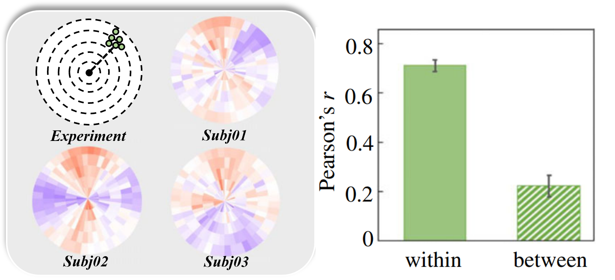
Figure 2. visual fingerprint experiments across subjects. ’Within’ denotes Pearson correlation coefficient of Distortion Indices in within-subject experiments, while ’between’ denotes between-subject.

4. Method

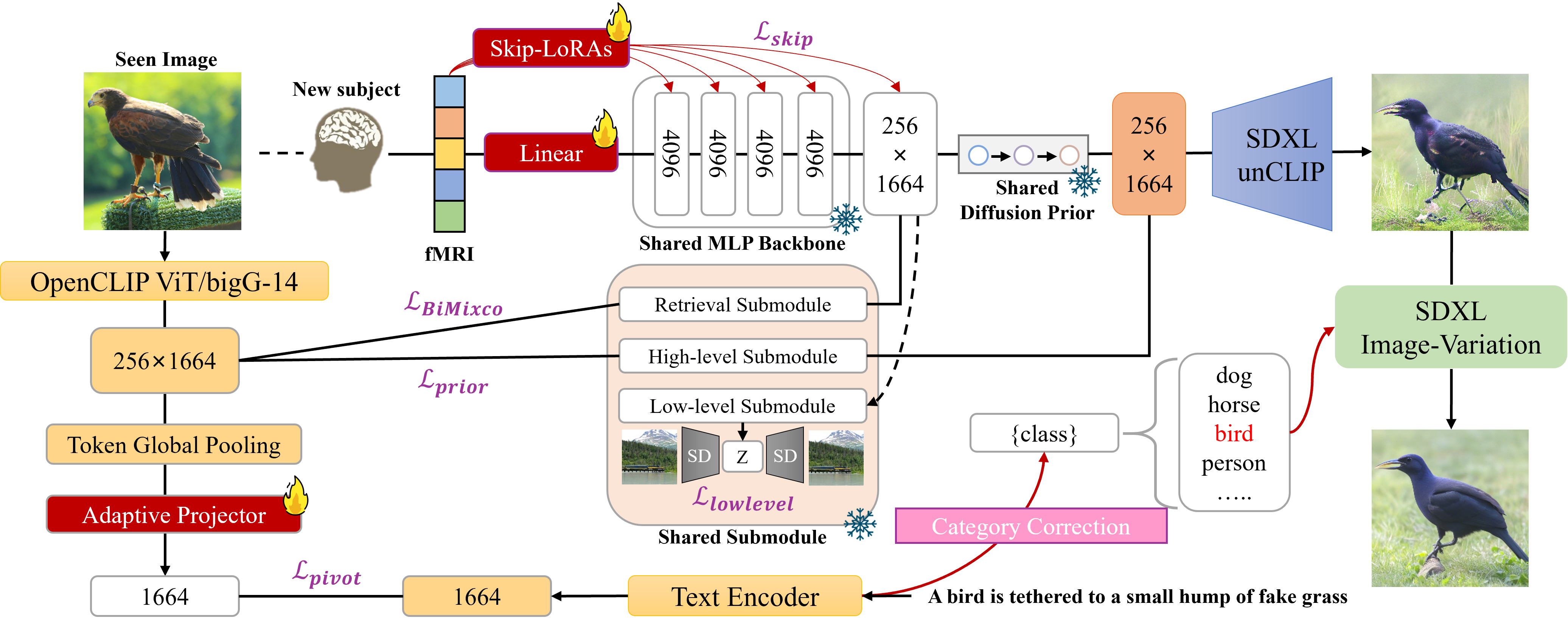
Figure 3. Schematic diagram of MindTuner for new-subject fine-tuning. All shared modules that have undergone multi-subject pre-training are frozen, including MLP Backbone, and submodules of retrieval, high-level, and low-level. The modules that need to be trained include Linear heads, Skip-LoRAs, Adaptive Projector, and LoRA blocks in linear layers. Images are reconstructed using diffusion prior and then SDXL, followed by semantic correction using SDXL Image-Variation.

The task of cross-subject visual decoding consists of two parts: multi-subject pre-training and new-subject fine-tuning. Given a neural dataset with brain activities of subject $s$, it involves the reconstruction of visual images $I\in\mathbb{R}^{3\times H\times W}$ through a core pipeline whose inputs are flattened and aligned fMRI voxels $V\in\mathbb{R}^{1\times d_{s}}$ after ROI extraction, where $d_{s}$ denotes voxel numbers. To simplify notation, each $(I,V)$ denotes data from original subjects for Section 4.1 and from new subjects for Section 4.2. Our goal is to optimize the $\mathcal{F(\cdot)}$, so that $\mathcal{F}(V)=\hat{I}$, where $\hat{I}$ best approximates $I$. New-subject fine-tuning adheres to the same path, albeit with scarce data. For the multi-subject pre-training, we follow the pipeline of MindEye2 (Scotti et al., 2024), while for the new-subject fine-tuning, we plug into visual fingerprint and Pivot as shown in Figure 3.

4.1. Multi-Subject Pre-training

4.1.1. Multi-Subject Functional Alignment

Note that different subjects have different brain structures and that the number of obtained voxels also varies. Therefore, a mapping model is needed to align the voxel inputs from different subjects to the same dimension as inputs to the model in the phase of multi-subject pre-training. Previous methods emphasized zero-shot using optimal transport models or few-shot using linear regression models. Here, we conduct linear function alignment to learn shared-subject fMRI latent space $M\in\mathbb{R}^{1\times d_{0}}$($d_{0}$ denotes shared input dimension) using subject-specific ridge regression as below:

(2) $$M=\textbf{Ridge}^{(s)}(V).$$

4.1.2. MLP Backbone

To perform high-fidelity pixel-level reconstruction, rich CLIP image embedding is needed. We use OpenCLIP ViT-bigG/14 for alignment whose image token embedding dimension is $256\times 1664$. Mapped inputs $M$ are fed into an MLP backbone with four residual blocks and a tokenization layer going from $d_{0}$-dim to $256\times 1664$. The MLP Backbone $\epsilon(\cdot)$ serves to convert the fMRI to the intermediate backbone embedding space: $Z=\epsilon(M)$. Note that all subjects shared the same MLP backbone after multi-subject functional alignment. Next, the backbone embeddings are passed into three submodules for retrieval, high-level reconstruction and low-level reconstruction.

4.1.3. Retrieval Submodules

To perform the retrieval task, a simple way is conducting a shallow mapping of the backbone embeddings and supervision with fMRI-to-image CLIP contrastive loss. For scarce fMRI samples, appropriate data augmentation helps model convergence. A recently effective voxel mixture paradigm based on MixCo (Kim et al., 2020) works well. Two raw fMRI voxels $V_{i}$ and $V_{j}$ are mixed into $V_{mix_{i,j}}$ using a factor $\lambda$ sampled from the Beta distribution:

(3) $$V_{mix_{i,j}} =\lambda_{i}V_{i}+(1-\lambda_{i})V_{j},$$

$$M_{mix_{i,j}} =\textbf{Ridge}^{(s)}(V_{mix_{i,j}}),$$

$$Z_{mix_{i,j}} =\epsilon(M_{mix_{i,j}}).$$

where $j$ denotes an arbitrary mixing index in the batch. The forward mixed contrastive loss MixCo is formulated as:

(4) $$\mathcal{L}_{MixCo}=-\frac{1}{|B|}\sum_{i=1}^{|B|}[\lambda_{i}\log\frac{\exp(Z_{mix_{i,j}}\cdot\ g_{i}/{\tau})}{\sum_{m=1}^{|B|}\exp(Z_{mix_{i,j}}\cdot\ g_{m}/{\tau})}$$

$$+(1-\lambda_{i})\log\frac{exp(Z_{mix_{i,j}}\cdot\ g_{j}/{\tau})}{\sum_{m=1}^{|B|}\exp(Z_{mix_{i,j}}\cdot g_{m}/{\tau})}],$$

where $g$ denotes ground-truth CLIP image embeddings, $\tau$ denotes a temperature hyperparameter, and $B$ is the batch size. Here we use the bidirectional loss $\mathcal{L}_{BiMixCo}$.

4.1.4. Low-level and High-level Submodules

Low-level pipeline is widely used to enhance low-level visual metrics in reconstruction images, which map voxels to the latent space of Stable Diffusion’s variational autoencoder (VAE) and is a ’guess’ for the reconstruction. It consists of a MLP and a CNN upsampler with L1 loss in Stable Diffusion’s latent space $z$.

(5) $$\mathcal{L}_{lowlevel}=\frac{1}{|B|}\sum_{i=1}^{|B|}|z_{i}-\hat{z_{i}}|.$$

On the other hand, high-level pipeline emphasizes pixel-wise alignment. Inspired by DALLE·2 (Ramesh et al., 2022), a diffusion prior is recognized as an effective means of transforming backbone embeddings into CLIP ViT image embeddings, in which mean square error loss is used:

(6) $$\mathcal{L}_{prior}=\frac{1}{|B|}\sum_{i=1}^{|B|}||g_{i}-\hat{g_{i}}||^{2}_{2}.$$

Thus, the end-to-end loss for multi-subject pre-training is:

(7) $$\mathcal{L}_{multi}=\mathcal{L}_{prior}+\alpha_{1}\mathcal{L}_{lowlevel}+\alpha_{2}\mathcal{L}_{BiMixCo}.$$

4.2. New-Subject Fine-tuning

4.2.1. Low-Rank Adaptation

Previous works have demonstrated the effectiveness of low-rank adaptation in large language model fine-tuning with significantly fewer trainable parameters. It is well matched to our cross-subject decoding task for two reasons. One is because most of the current mainstream models for decoding fMRI are MLP-based models, which contain a large number of linear layers, while LoRA has also been shown to achieve good fine-tuning results in the linear layers. Second, in cross-subject scenarios, fMRI data from new subjects are usually scarce, and full-tuning the whole model is usually difficult to grasp, leading to a certain degree of overfitting. For each pre-trained weight matrix $\in\mathbb{R}^{d_{in}\times d_{out}}$ in the multi-subject model, where $d_{in}$ denotes input dimension and $d_{out}$ denotes output dimension, gradient update is constrained with a low-rank decomposition for new-subject adapter matrix $\Delta W$:

(8) $$W+\Delta W=W+BA,$$

where $W$ is keeped frozen, $B\in\mathbb{R}^{d_{out}\times r}$, $A\in\mathbb{R}^{r\times d_{in}}$, $r$ is the rank and $r\ll min(d_{in},d_{out})$. At the beginning of the training phase, the parameters of the matrix $B$ are randomly initialized, and $A$ is initialized to zero, which ensures that the initial output of the LoRA block is all zeros.

4.2.2. non-linear Skip-LoRAs

Although LoRA is an effective means of fine-tuning multi-subject models. However, there exists a non-linear relationship between subjects (discussed in Section 3), and the visual fingerprint of new subjects can not be totally obtained with linear models like LoRA. Previous methods selected linearly aligned multi-subjects and abandoned exploring non-linear relationships because of the low signal-to-noise ratio of fMRI. Thus, overly complex non-linear alignment models can lead to models overfitting fMRI noise. LoRA is a very lightweight model and well circumvents complexity, so we simply need to add non-linear constraints to LoRA blocks. Here, we design our non-linear LoRAs by adding the activation function and the non-linear correlation loss to the output of LoRAs. Inspired by the skip-connection of Unet in Computer Vision (Zhang et al., 2023), we design a new non-linear Skip-LoRAs to bootstrap the initial non-linearity of fMRI between subjects directly affecting the entire MLP backbone(see Appendix A.2 for Skip-LoRAs). Skip-LoRAs can be defined as $\textbf{Skip-LoRA}=Activation(BA)$. Assuming that $\epsilon_{h}(\cdot)$ is the $h$-th layer of MLP backbone $\epsilon(\cdot)$, the output of new-subject backbone $M_{h}$ could be as follows:

(9) $$M_{0}=\textbf{Ridge}^{(s)}(V),$$

$$M_{h}=M_{h-skip}+M_{h-linear},$$

$$M_{h-linear}=\epsilon_{h}(M_{h-1})+\textbf{LoRA}_{h}(M_{h-1}),$$

$$M_{h-skip}=\textbf{Skip-LoRA}_{h}(V).$$

Here, we use Pearson correlation coefficient to define the non-linear correlation loss:

(10) $$\mathcal{L}_{skip}=\frac{1}{|B|}\frac{1}{|H|}\sum_{i=1}^{|B|}\sum_{h=1}^{|H|}|Pearson(M_{h-linear},M_{h-skip})|.$$

4.2.3. Pivot with Adaptive Projector

In addition to pixel-level alignment, semantic-level matching is equally important for reconstructing the semantic integrity of an image. In visual decoding tasks, fMRI is directly associated with the image stimulus, and semantic information is implicit in fMRI. Here, we offer a new fMRI-to-text alignment inspired by the structure of ViT and CLIP contrastive learning. In image-text contrastive learning, the last projection layer of ViT is responsible for mapping tokens to the same dimension as the text (e.g., $1280$ in OpenCLIP ViT-bigG/14). This mapping is done after directly mapping the CLS token or all 257 tokens with global average pooling in the penultimate layer. Here, we use all 256 tokens, excluding the CLS token, which is the input of MindEye2’s SDXL Unclip. In order to accommodate the scarcity of fMRI data during few-shot learning across subjects, we fine-tuned our adaptive projector from the OpenCLIP ViT-bigG/14 of 256 tokens on the MSCOCO dataset, which consists of 73k images and 5 texts in each image. For new subjects, we add the additional image-text loss to the model to constrain the semantic information of aligned 256 tokens:

(11) $$\mathcal{L}_{pivot}=-\frac{1}{|B|}\sum_{i=1}^{|B|}\log\frac{\exp(p_{i}\cdot\ t_{i}/{\tau})}{\sum_{m=1}^{|B|}\exp(p_{i}\cdot\ t_{m}/{\tau})},$$

where $p$ denotes projector’s output from image tokens $g$, and $t$ denotes the CLS embeddings of paired text. During new-subject fine-tuning, the adaptive projector is trainable. Thus, the end-to-end loss for new-subject fine-tuning is:

(12) $$\mathcal{L}_{new}=\mathcal{L}_{multi}+\alpha_{3}\mathcal{L}_{skip}+\alpha_{4}\mathcal{L}_{pivot}.$$

4.2.4. Semantic Correction

MindEye2 has found that the reconstruction images from SDXL UnCLIP after aligning tokens have fuzzy semantics, so the aligned embeddings are fed into the image captioning model GIT (Wang et al., 2022) to get the semantics for refinement. We have found that single category words are sufficient to accomplish the refinement task. In addition, the captions generated by MindEye2 are completely dependent on aligned embeddings, which can only make the image semantics clearer and cannot correct the semantics of the reconstruction images, as shown in Figure 4. Benefiting from our adaptive projector, we can define category description as fMRI-to-text retrieval tasks using a simple text promt $[class]$. In this way, we achieve more accurate category reconstruction.

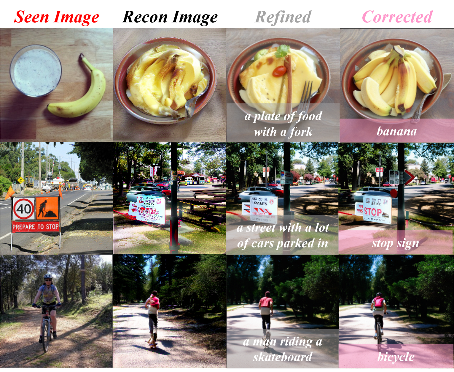
Figure 4. SDXL unCLIP reconstructions and SDXL Image-Variation by MindEye2’s refinement or our correction.

Method	Low-Level				High-Level				Retrieval
	PixCorr$\uparrow$	SSIM$\uparrow$	Alex(2)$\uparrow$	Alex(5)$\uparrow$	Incep$\uparrow$	CLIP$\uparrow$	Eff$\downarrow$	SwAV$\downarrow$	Image$\uparrow$	Brain$\uparrow$
Takagi… (Takagi and Nishimoto, 2023)	0.246	0.410	78.9%	85.6%	83.8%	82.1%	0.811	0.504	-	-
Ozcelik… (Ozcelik and VanRullen, 2023)	0.273	0.365	94.4%	96.6%	91.3%	90.9%	0.728	0.422	18.8%	26.3%
MindEye1 (Scotti et al., 2023)	0.319	0.360	92.8%	96.9%	94.6%	93.3%	0.648	0.377	90.0%	84.1%
MindEye2 (Scotti et al., 2024)	0.322	0.431	96.1%	98.6%	95.4%	93.0%	0.619	0.344	98.8%	98.3%
MindTuner(Ours)	0.322	0.421	95.8%	98.8%	95.6%	93.8%	0.612	0.340	98.9%	98.3%
MindEye2(1 hour) (Scotti et al., 2024)	0.195	0.419	84.2%	90.6%	81.2%	79.2%	0.810	0.468	79.0%	57.4%
MindTuner(1 hour)	0.224	0.420	87.8%	93.6%	84.8%	83.5%	0.780	0.440	83.1%	76.0%

Table 1. Quantitative comparison of MindTuner reconstruction performance against other methods. All results are averaged across subjects 1, 2, 5 and 7 from the Natural Scenes Dataset. The results of other methods are taken from MindEye2(Scotti et al., 2024), using either 40 hour data or 1 hour data. Some methods were not included in the comparison because they used past 37 hour data and were not open-source. Missing values occur when metrics are not applicable. Bold font signifies the best performance, while underlined text indicates the second-best performance. See Appendix A.1 for a detailed description of the evaluation metrics.

5. Experiment

5.1. Datasets

Natural Scenes Dataset (NSD) (Allen et al., 2022) is an extensive 7T fMRI dataset gathered from 8 subjects viewing images on the MSCOCO-2017 dataset, containing images of complex natural scenes. Participants viewed three repetitions of 10,000 images with a 7-Tesla fMRI scanner over 30–40 sessions, with one session including 750 fMRI trials lasting for about 1 hour. More details can be found on the NSD official website. Our new-subject experiments focused on Subj01, Subj02, Subj05, and Subj07, who finished all viewing trials and are the subjects used in previous research (Ozcelik and VanRullen, 2023; Scotti et al., 2023, 2024; Takagi and Nishimoto, 2023), and our multi-subject experiments used the remaining 7 subjects. Each subject’s training set comprises 9000 image stimuli and 27000 fMRI trials (with 3 repetitions per image). The test set contains 1000 image stimuli and 3000 fMRI trials, which are averaged across trials. By applying the nsdgeneral ROI mask with a 1.8 mm resolution, we obtained ROIs for subjects. These regions span visual areas ranging from the early visual cortex to higher visual areas.

Note that all previous work, excluding MindEye2, did not use the full 40 sessions of NSD data, which was released in the recent completion of the 2023 Algonauts challenge. In this paper, we parallel the MindEye2’s setup.

5.2. Implementation details

All our fine-tuning experiments were conducted for 150 epochs on two Tesla v100 32GB GPUs, with batch size set to 10. The experimental parameter settings for 1 hour and 40 hour data are consistent. For fine-tuning experiments, the loss weight is set to $[\alpha_{1},\alpha_{2},\alpha_{3},\alpha_{4}]=[0.5,1.0,1.5,0.5]$ and for all LoRA blocks, including Skip-LoRAs, rank $r$ is set to 8. We use the AdamW (Loshchilov and Hutter, 2017) for optimization, with a learning rate set to 3e-4, to which the OneCircle learning rate schedule (Smith and Topin, 2019) was set. During the training process, we use data augmentation from images and blurry images and replace the BiMixCo with SoftCLIP (Scotti et al., 2023) loss in one-third of the training phase. In the inference stage, we only generated a reconstructed image once and did not make multiple selections. The final high-level reconstructed image and low-level blurry image are simply weighted and averaged in a ratio of 3:1. In the inference stage of semantic correction, we use 80 category nouns from MSCOCO as correction texts and classify them in the form of text retrieval.

6. Results and Analysis

6.1. Image and Brain Retrieval

Image retrieval refers to retrieving the image embeddings with the highest cosine similarity based on voxel embeddings on the test set. If a paired image embedding is retrieved, the retrieval is considered correct. Brain retrieval is the opposite process mentioned above. Previous work has shown that image retrieval can be an efficient way to assist with fine-grained pixel-level alignment (Scotti et al., 2024, 2023; Xia et al., 2024). Following their approach, we set the size of the retrieval pool to 300. For each test sample, we randomly selected 299 images from the remaining 999 images on the test set and calculated the cosine similarity between the voxel embeddings and 300 image embeddings. The retrieval accuracy refers to the proportion of successful retrieval of corresponding images in the 1000 voxel embeddings of the test set. We adjusted the random number seed of 30 randomly selected images to average the accuracy of all samples. In Table1, there is only an extremely slight improvement in retrieval accuracy when having fMRI data within 40 hours. This may be attributed to the fact that the retrieval accuracy is already close to the upper limit (only about 1% short of reaching 100%), which is affected by the noise of the fMRI dataset itself. However, when only 1 hour of data was available, MindTuner’s retrieval accuracy was significantly higher than MineEye2, 4.1% higher for image retrieval and 18.6% higher for brain retrieval. As MindEye2 benefits from multi-subject pre-training and new-subject fine-tuning with linear heads, this indicates that our introduced visual fingerprint greatly improve the performance of the model when fMRI data is scarce.

6.2. Text Retrieval

As with the image/brain retrieval in the above section, text retrieval refers to finding the text description that best describes the stimulus image according to fMRI. Since the subjects were not exposed to textual stimuli, we did not use the previous method of directly aligning fMRI to the text. Instead, we utilized the relationship between image tokens and text tokens to indirectly connect fMRI and text. During the training phase, we randomly selected one of the 5 captions from each image, while during the testing phase, we randomly selected a fixed caption for testing. Due to the significant similarity in text descriptions, even the text ground truth of two different images can describe each other. Thus, we only reported text retrieval accuracy of the top 5 in Table 2. In addition to the same better improvement in 1 hour data, the retrieval accuracy of 40 hours has also been improved, indicating the reliability of the adaptive projector. What’s more, better projectors provide a foundation for subsequent semantic correction.

Method	Subj01	Subj02	Subj05	Subj07	Avg
MindEye2(1 hour)	13.6%	10.7%	12.5%	6.9%	10.9%
MindTuner(1 hour)	17.7%	14.4%	18.9%	13.5%	16.1%
MindEye2(40 hours)	45.4%	38.8%	49.3%	39.8%	43.3%
MindTuner(40 hours)	47.3%	41.7%	52.0%	42.5%	45.9%

Table 2. fMRI–image-text retrieval perfomance(aka top-5 retrieval performance, chance=5/1000). The reported methods all used our pre-trained projectors, while MindEye2 includes frozen projectors, and MindTuner uses adaptive projectors. See the Appendix B.1 for the effectiveness of pre-tained projectors on the MSCOCO.

6.3. Reconstruction

Image reconstruction aims to restore the original image as seen by the subjects, and two levels of evaluation metrics rate the quality of the reconstructions. The low-level metrics are designed to examine the pixel-level similarity between the generated image and the original image, which is related to low-level human vision, while the high-level metrics consider the semantic correlation between the generated image and the original one, which is more closely related to the higher visual cortex. Previous researches have improved the performance of these above metrics in single-subject models by various means. The cross-subject task discussed in this paper tests the model’s ability to draw on the commonalities of multi-subject and to migrate new subjects, ultimately realizing the goal of using fewer fMRI data for few-shot learning. Here, we report the reconstruction results of MindTuner using training data of 1 hour and 40 hours. Table 1 reflects the quantized performance comparisons, under two different training data sizes. It can be seen that when using the full NSD dataset, MindTuner achieves better performance on high-level metrics; when only 1 hour of data is available for training, MindTuner outperforms MindEye2 on all metrics. The visualization results of 1 hour and 40 hours reconstructions can be seen in Figure 5 and Figure 6. It can be seen that the quality of the reconstructed images is significantly higher at 40 hours than at 1 hour as the training data increases. Meanwhile, our MindTuner is better than MindEye2 in both semantic completeness and category accuracy, proving the superiority of the overall model. Our visualization excludes the other three methods in Table 1 because the image semantics generated by these three methods are very unclear. Interestingly, we also found that images generated directly from SDXL Unclip outperformed MindEye2 refined and MindTuner corrected images at the high-level, though visibly distorted. More details can be found in Appendix B.2.

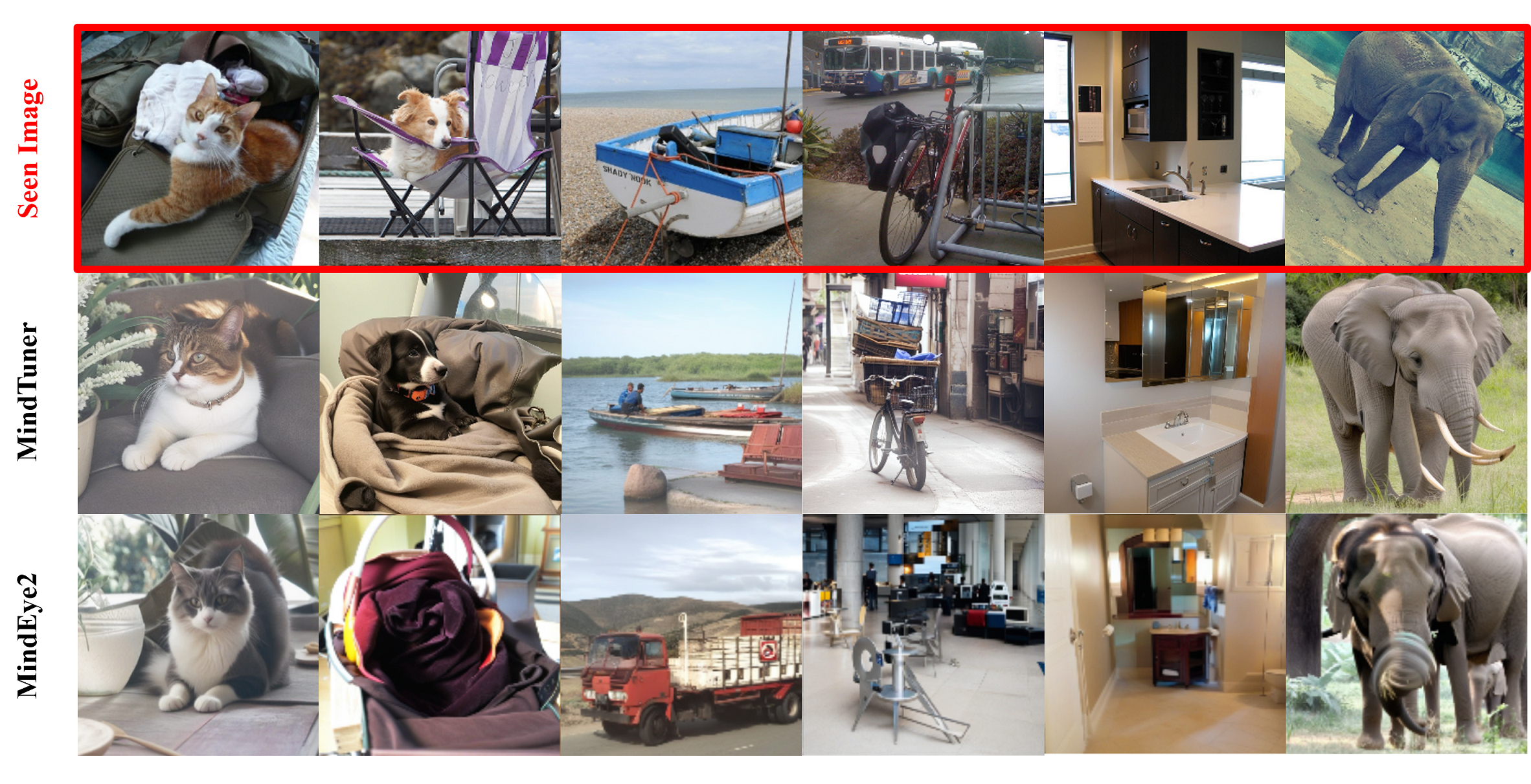
Figure 5. MindTuner vs MindEye2 reconstructions from fMRI brain activity with only 1 hour of data.

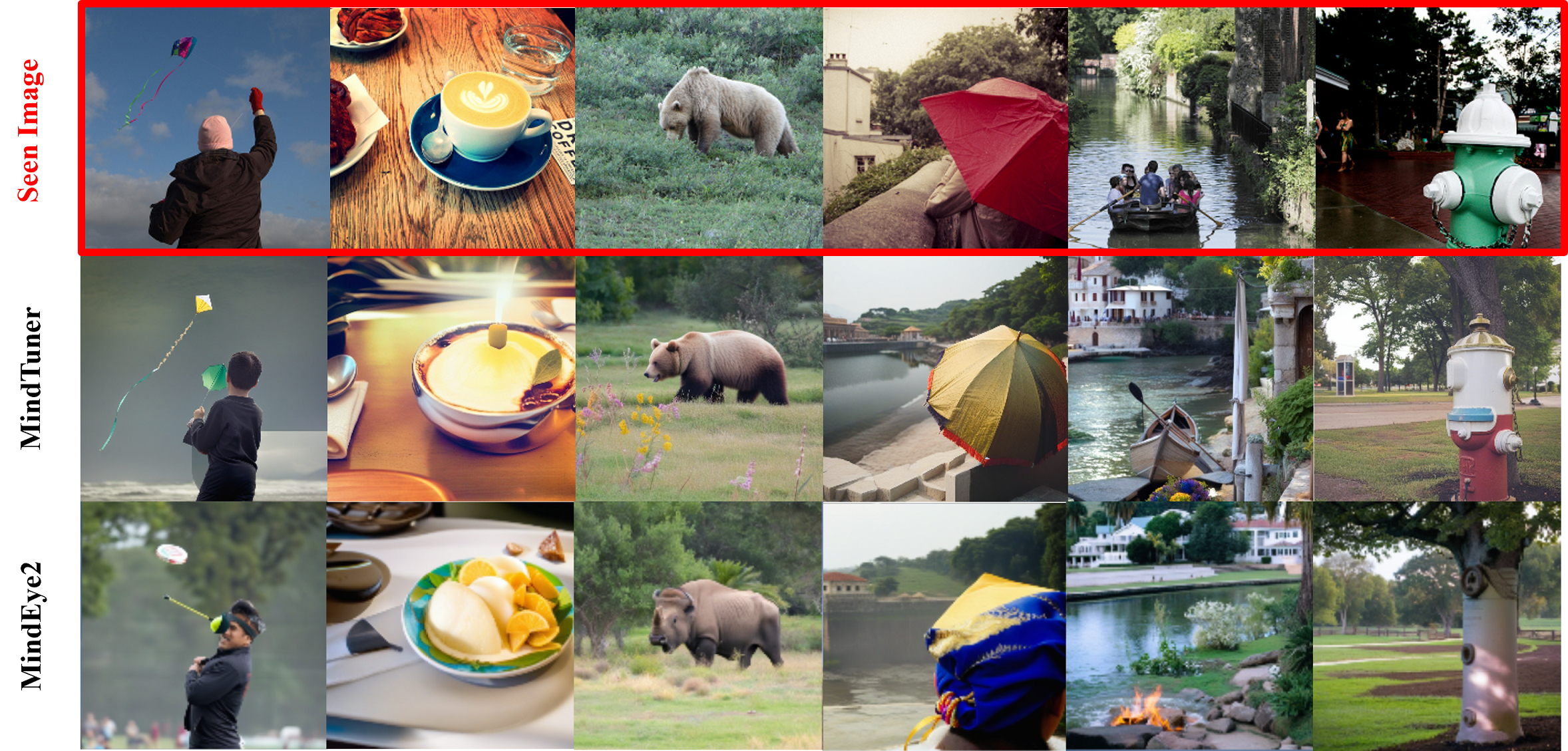
Figure 6. MindTuner vs MindEye2 reconstructions from fMRI brain activity with 40 hours of data.

6.4. Brain Correlation

In addition to evaluating the quality of images from the perspective of reconstruction itself, recent studies (Scotti et al., 2023; Kneeland et al., 2023) have also interestingly examined the process of encoding images into fMRI to determine whether reconstructed images can elicit similar fMRI responses. The encoding model can provide a measure of similarity between images and brain responses with the visual forward encoding pathway of fMRI. Furthermore, the encoding model can evaluate the reconstruction quality in the presence of unknown ground-truth images, and the brain correlation metrics it brings can also measure the degree to which the model fits the consistency of human observers. We used the same brain coding model GNet (St-Yves et al., 2022; Kneeland et al., 2023) as previous researchers to calculate brain correlation metrics, and the results are shown in Table 8. The table clearly demonstrates that MindTuner maintains a higher brain correlation than MindEye2 within the V1-V4 region. This suggests that while there’s a shared encoding approach among subjects, each individual possesses distinct encoding patterns(i.e., visual fingerprint). With the introduction of MindTuner’s visual fingerprint and semantic correction, there’s an opportunity for subjects to develop personalized encoding strategies autonomously. The results in the table are all based on training data of 40 hours, and the brain correlation coefficients of the 1 hour data are shown in Appendix B.3.

Brain Region	MindTuner	MindEye2 (Scotti et al., 2024)	Ozcelik.. (Ozcelik and VanRullen, 2023)	Takagi.. (Takagi and Nishimoto, 2023)
Visual cortex$\uparrow$	0.377	0.373	0.381	0.247
V1$\uparrow$	0.367	0.364	0.362	0.181
V2$\uparrow$	0.355	0.352	0.340	0.152
V3$\uparrow$	0.346	0.342	0.332	0.152
V4$\uparrow$	0.330	0.327	0.323	0.170
Higher vis.$\uparrow$	0.372	0.368	0.375	0.288

Table 3. The brain correlation scores computed across various brain regions, encompassing the visual cortex, early visual cortical areas such as V1, V2, V3, and V4, as well as higher visual regions (Visual cortex denotes the ROI of nsdgeneral).

Method	Trainable	Low-Level				High-Level				Retrieval
	Parameters	PixCorr$\uparrow$	SSIM$\uparrow$	Alex(2)$\uparrow$	Alex(5)$\uparrow$	Incep$\uparrow$	CLIP$\uparrow$	Eff$\downarrow$	SwAV$\downarrow$	Image$\uparrow$	Brain$\uparrow$
MindEye2	64.4M(-)	0.235	0.428	88.0%	93.3%	83.6%	80.8%	0.798	0.459	94.0%	77.6%
with Adaptive Projector	66.5M(+2.1M)	0.233	0.426	87.8%	93.0%	84.0%	81.2%	0.794	0.454	93.8%	77.3%
with only LoRAs	74.6M(+9.4M)	0.261	0.427	90.3%	94.2%	84.8%	84.0%	0.784	0.441	93.7%	85.6%
LoRAs+Skip-LoRAs	74.6M(+10.2M)	0.264	0.427	90.8%	94.8%	85.1%	84.2%	0.780	0.437	94.5%	87.7%
MindTuner(non-linear)	76.7M(+12.3M)	0.191	0.383	82.7%	88.0%	77.3%	76.0%	0.848	0.492	27.4%	56.7%
MindTuner	76.7M(+12.3M)	0.262	0.422	90.6%	94.9%	85.8%	84.6%	0.774	0.433	94.2%	87.4%

Table 4. Ablations on the modules of MindTuner. Note that all model parameters for MindEye2 are 2.2B, and we only reported the trainable parameters required for new-subject fine-tuning. MinTuner(non-linear) denotes adding an activation function to ridge regreesion head.

$rank$	Trainable	Skip-LoRAs	Low-Level				High-Level				Retrieval
	Parameters	Parameters	PixCorr$\uparrow$	SSIM$\uparrow$	Alex(2)$\uparrow$	Alex(5)$\uparrow$	Incep$\uparrow$	CLIP$\uparrow$	Eff$\downarrow$	SwAV$\downarrow$	Image$\uparrow$	Brain$\uparrow$
$4$	71.6M(+7.2M)	0.4M	0.263	0.422	90.4%	94.9%	84.8%	84.6%	0.778	0.436	94.4%	87.9%
$8$	76.7M(+12.3M)	0.8M	0.262	0.422	90.6%	94.9%	85.8%	84.6%	0.774	0.433	94.2%	87.4%
$16$	86.7M(+22.3M)	1.6M	0.262	0.422	90.5%	95.1%	85.2%	85.2%	0.776	0.434	93.7%	87.2%

Table 5. Ablations on the rank $r$ of MindTuner.

7. Ablations

In this section, we explored the effectiveness of each component of our method through ablation experiments. All results were pre-trained on Subjects 2-8, and fine-tuning was performed on Subject 1 using 1 hour of data.

Effect of MindTuner’s modules. We conducted additional experiments to evaluate the effectiveness of each module. From Table 4, it can be seen that the introduction of LoRAs greatly improves the model’s ability. When Skip-LoRAs are added, all image reconstruction metrics approach the entire model, and the retrieval accuracy even exceeds the complete model. This may be due to the balance of additional image-to-text aligned losses, which slightly reduces the performance of the retrieval submodule in the complete model. Meanwhile, the introduction of adaptive projector has improved the performance of high-level visual reconstruction, and more visualizations in Figure 4 have also shown the effectiveness of semantic correction, but it will sacrifice some low-level effects. Overall, compared to the 2.2B multi-subject pre-trained main model, MindTuner only increased the parameter count by 12.3M, achieving better results. We also add an activation function to the ridge head to make the whole alignment head non-linear, and the 76.7M non-linear head brings a serious overfitting phenomenon, with all metrics seriously degrading. It shows that the overly large non-linear model is not suitable for the fMRI alignment of these different subjects, while visual fingerprint in MindTuner is a better choice.

Effect of the rank $r$ of Skip-LoRAs and LoRAs. We conducted extra experiments on the most critical variable in the LoRAs, the size of the rank $r$. As shown in Table 5, it can be seen that when the rank $r=4/16$ , the overall ability of the model does not show significant changes. This is consistent with the results studied in the LoRA paper (Hu et al., 2021), which pointed out that when $r\in[2,16]$, the fine-tuning effect is basically the same. In addition, no significant overfitting was observed, probably because parameters in Skip-LoRAs have remained relatively small, consistently under 2M.

8. Neuroscience interpretability

To investigate the interpretability of MindTuner in neuroscience, we conduct experiments to explore where the subject’s non-linear relationship comes from in the visual cortex. We utilize pycortex (Gao et al., 2015) to project the weights of each voxel in the first layer of linear ridge regression head, LoRA, or Skip-LoRA onto the corresponding 2D flat map of the NSD dataset. Results are in the Figure 7. It can be seen that for linear heads, the importance of visual cortical voxels is similar for both ridge and LoRA. However, for Skip-LoRA, a small portion of the early visual cortex and more advanced visual cortex are valued more. This indicates that at the fMRI level, a greater concentration of non-linear relationships is found within the higher visual cortex. It also demonstrates that the design of Skip-LoRAs is capable of capturing non-linear relationships in fMRI data that are not discernible with standard LoRAs. More visualization results, as well as brain region ROI templates, can be found in Appendix C.

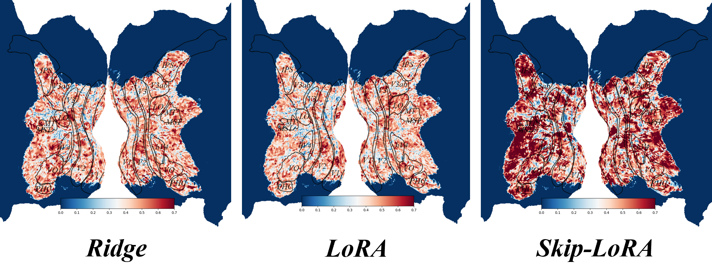
Figure 7. The importance of different ROIs of subject 1 with fitted weights of the first layer. The weights of each module are averaged and normalised between 0 and 1.

9. Limitations and Future Work

Although we introduced the visual fingerprint among subjects, we did not explore where the boundary of the degree of non-linearity between subjects lies. As is well known, overly complex non-linear models can fit into fMRI noise, while linear models can overlook the non-linear relationships between subjects. Therefore, a model that can be well balanced is a future research direction. In addition, we observe that during semantic correction, the single-category classification results of images depend more on the more salient objects in the natural scene. This leads MindTuner to correct only part of the semantic information of the reconstructed image. How to achieve fine-grained text control with more sophisticated forms of pivot, is also a direction for future thinking.

10. Conclusion

In this paper, we propose MindTuner, a new cross-subject decoding method. We introduced the phenomenon of visual fingerprint in the human visual system and utilized the combination of Skip-LoRAs and LoRAs to learn each subject’s visual fingerprint. Meanwhile, we innovatively propose a method for enhancing reconstruction images by indirectly connecting fMRI with text in visual decoding tasks. Experimental results have shown that we have achieved better performance on multiple evaluation metrics at a relatively small parameter cost, especially when the fMRI data is insufficient. Our work has relaxed the conditions for fMRI acquisition, helping to achieve a universal brain decoding model in the future.

Appendix A Additional Details

A.1. Evaluation Metrics

Retrieval: Image retrieval refers to retrieving the image embeddings with the highest cosine similarity based on voxel embeddings on the test set(chance=0.3%). If a paired image embedding is retrieved, the retrieval is considered correct. Brain retrieval is the opposite process mentioned above.

PixCorr: pixel-wise correlation between ground truth and reconstructions;

SSIM: structural similarity index metric (Wang et al., 2004) between ground truth and reconstructions;

Eff (Tan and Quoc, [n. d.])and Swav (Caron et al., 2020) refer to average correlation distance with EfficientNet-B1 and SwAV-ResNet50.

Alex(2), Alex(5), Incep, CLIP: all these metrics refer to two-way identification (chance = 50%) using different models. The two-way comparisons were performed with AlexNet where Alex(2) denotes the second layer and Alex(5) denotes the fifth layer, InceptionV3 with the last pooling layer, and CLIP with th final layer of ViT-L/14. Two-way identification refers to percent correct across comparisons gauging if the original image embedding is more similar to its paired voxel embedding or a randomly selected voxel embedding. We followed the same image preprocessing and the same two-way identification steps as  (Ozcelik and VanRullen, 2023; Scotti et al., 2023, 2024). For each test sample, performance was averaged across all possible pairwise comparisons using the other 999 reconstructions to ensure no bias from random sample selection. This yielded 1,000 averaged percent correct outputs.

A.2. Skip-LoRAs

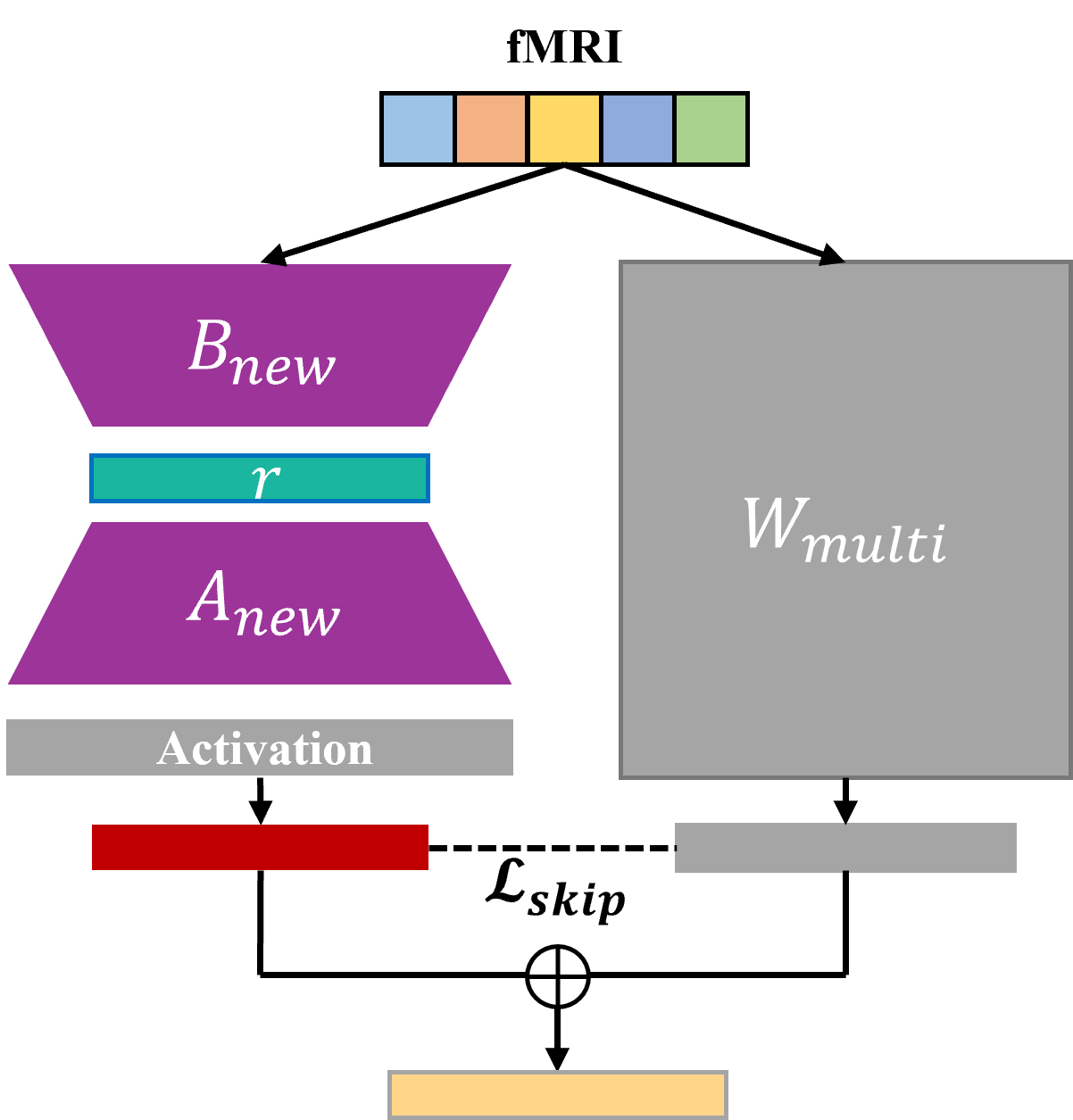
Figure 8. Design of Skip-LoRAs. $W_{multi}$ denotes shared weight during multi-subject pre-training. A Skip-LoRA block consists of a LoRA block with skip-connection, activation function, and non-linear loss $\mathcal{L}_{skip}$

As described in the main text, we designed Skip-LoRAs to better learn visual fingerprint between subjects, especially the non-linear part. The structure of Skip-LoRAs is shown in Figure 8. The pre-trained shared model of the MLP Backbone includes an alignment layer that aligns voxels to 4096-dim, four 4096-dim residual blocks and a layer that maps to image tokens. We used Skip-LoRAs to connect fMRI to these layers, allowing the initial fMRI differences to affect the entire network. $\mathcal{L}_{skip}$ was also used for these connections, except for the last mapping layer of image tokens, as the non-linear constraints and retrieved cosine similarity-based contrastive loss conflicted with each other.

Appendix B Additional Results

B.1. Adapative Porjector pre-trained on MSCOCO

Previous CLIP-related articles have demonstrated that ViT’s projection layer can take both CLS tokens and the result of global average pooling of all tokens as inputs. We perform a global average pooling of all 256 brain tokens, which finally are mapped to the same 1280 dimensions as the CLS token of the text. The PyTorch code used to train the projector is depicted below:

⬇

class Adaptive_Projector(torch.nn.Module):

def __init__(self):

super().__init__()

self.proj = nn.Parameter(

torch.randn(1664, 1280))

def forward(self, x):

x = torch.mean(x, dim = 1)

x = x @ self.proj

return x

We trained this projection layer on the whole COCO 2017 dataset including 73k images and 5 texts for each image. We randomly selected 900 image-text pairs as the validation set, and used a retrieval pool of 300 for validation (a similar setup to our main experiment). Instead of training from scratch, we used the projection layer of image CLS token from the open-source OpenCLIP to start fine-tuning for 20 epochs, with the learning rate being fixed at 3e-4 and the batch size at 512. The loss is the standard CLIP image-text contrastive loss. The accuracy of validation set retrieval before and after fine-tuning is as follows:

Method	Image2Text	Text2Image
Before fine-tuning	81.3%	78.7%
After fine-tuning	95.2%	95.2%

Table 6. Fine-tuning results on the COCO 2017.

Method	Data Size	Low-Level				High-Level
		PixCorr$\uparrow$	SSIM$\uparrow$	Alex(2)$\uparrow$	Alex(5)$\uparrow$	Incep$\uparrow$	CLIP$\uparrow$	Eff$\downarrow$	SwAV$\downarrow$
MindTuner(Uncorrected)	40 hours	0.280	0.327	95.4%	99.2%	96.4%	94.5%	0.621	0.341
MindTuner	40 hours	0.322	0.421	95.8%	98.8%	95.6%	93.8%	0.612	0.340
MindTuner(Uncorrected)	1 hour	0.208	0.378	87.4%	94.0%	85.5%	83.8%	0.781	0.439
MindTuner	1 hour	0.224	0.420	87.8%	93.6%	84.8%	83.5%	0.780	0.440

Table 7. Quantitative effects on semantic correction.

B.2. Semantic Correction Influence

As shown in Figure 7, we observe that semantic correction, while making the semantics of the reconstructed images clearer and more accurate, negatively affects the evaluation metrics, especially high-level. This is similar to MindEye2’s results, suggesting that manual correction of the image, either by MindEye2’s refinement or MindTuner’s correction, can have an adverse effect on the original fMRI representation. And as can be seen in Table 1, MindTuner mitigates this negative effect to some extent, compared to MindEye2.

B.3. Additional Brain Correlation Reults

The Brain Correlation results with 1-hour data is as follows. In conjunction with Table 3, it can be seen that MindTuner greatly improves the brain correlation of the reconstructed images, especially when the data is scarce. It suggests that the learning of subjects’ visual fingerprint preserves their own properties to some extent.

Brain Region	MindTuner	MindEye2 (Scotti et al., 2024)
Visual cortex$\uparrow$	0.372	0.348
V1$\uparrow$	0.345	0.309
V2$\uparrow$	0.348	0.314
V3$\uparrow$	0.347	0.315
V4$\uparrow$	0.329	0.300
Higher vis.$\uparrow$	0.370	0.351

Table 8. The brain correlation scores computed across various brain regions with 1 hour data.

1-hour data   —		Subject 1	Subject 2	Subject 5	Subject 7
Low-Level	PixCorr$\uparrow$	0.262	0.225	0.208	0.202
	SSIM$\uparrow$	0.422	0.425	0.415	0.417
	Alex(2)$\uparrow$	90.6%	89.1%	86.8%	84.5%
	Alex(5)$\uparrow$	94.9%	95.1%	93.7%	90.8%
High-Level	Incep$\uparrow$	85.8%	84.8%	87.7%	80.7%
	CLIP$\uparrow$	84.6%	83.7%	85.9%	79.6%
	Eff$\downarrow$	0.774	0.781	0.750	0.817
	SwAV$\downarrow$	0.433	0.440	0.422	0.465
Retrieval	Image$\uparrow$	94.2%	93.7%	72.2%	71.9%
	Brain$\uparrow$	87.4%	82.8%	68.1%	65.5%
Brain	Visual cortex$\uparrow$	0.359	0.376	0.426	0.328
	V1$\uparrow$	0.336	0.342	0.366	0.335
Correlation	V2$\uparrow$	0.354	0.326	0.373	0.339
	V3$\uparrow$	0.355	0.348	0.354	0.329
	V4$\uparrow$	0.327	0.366	0.328	0.294
	Higher vis.$\uparrow$	0.358	0.379	0.432	0.311

Table 9. Specific subject quantitative results with 1-hour training data.

40-hours data   —		Subject 1	Subject 2	Subject 5	Subject 7
Low-Level	PixCorr$\uparrow$	0.371	0.331	0.298	0.288
	SSIM$\uparrow$	0.428	0.421	0.422	0.414
	Alex(2)$\uparrow$	97.7%	96.8%	94.7%	94.1%
	Alex(5)$\uparrow$	99.3%	99.0%	98.7%	98.1%
High-Level	Incep$\uparrow$	96.4%	95.1%	96.6%	94.1%
	CLIP$\uparrow$	94.3%	92.7%	94.7%	93.3%
	Eff$\downarrow$	0.601	0.620	0.592	0.636
	SwAV$\downarrow$	0.331	0.342	0.333	0.355
Retrieval	Image$\uparrow$	100%	99.9%	98.4%	97.2%
	Brain$\uparrow$	99.9%	99.8%	96.8%	96.6%
Brain	Visual cortex$\uparrow$	0.377	0.394	0.416	0.320
	V1$\uparrow$	0.387	0.400	0.357	0.323
Correlation	V2$\uparrow$	0.381	0.359	0.361	0.317
	V3$\uparrow$	0.366	0.373	0.341	0.302
	V4$\uparrow$	0.340	0.376	0.324	0.278
	Higher vis.$\uparrow$	0.363	0.387	0.426	0.311

Table 10. Subject’s specific quantitative results with 40-hours training data.

B.4. Subject’s Specific Results

Tables 9 and 10 show more exhaustive evaluation metrics computed for every subject individually using 40-hours and 1-hour of fine-tuning data respectively. It can be seen that the performance of different subjects is relatively similar regardless of the amount of data, e.g., Subject 1 performs better at the low-level and retrieval, while Subject 5 performs better at the high-level.

B.5. Subject’s Specific Visualizations

We visualize in Figure 11 and Figure 12 the specific reconstruction results for different subjects, using either 1-hour or 40-hours data. For different subjects, MindTuner’s reconstructed images were accurate in capturing semantics, but the details varied. This may be attributed to the fact that the CLIP representation space is more semantic than detailed texture. In addition to this, as the training data increases, the blurry images become more similar to the ground truth images, thus giving a boost to the low-level metrics, as shown in Tables 11 and 12. Unfortunately, the color distribution of blurry images and reconstructed images is often difficult to control, e.g., generating airplanes of various colors. We have tried to add a sub-module to align the fMRI to a $16\times 16$ spatial palette, but the spatial palettes obtained are only slightly better than the blurry images. Moreover, the T2I Adapter generation model based on spatial palette is difficult to control, which often makes the reconstruction results even worse. Thus, the relationship between the visual system and color needs to be further explored.

B.6. COCO Category

There are 80 categories of object categorization in MSCOCO, and the category text was used by us for semantic correction in MindTuner, below are the 80 categories:

’person, bicycle, car, motorcycle, airplane, bus, train, truck, boat, traffic light, fire hydrant, stop sign, parking meter, bench, bird, cat, dog, horse, sheep, cow, elephant, bear, zebra, giraffe, backpack, umbrella, handbag, tie, suitcase, frisbee, skis, snowboard, sports ball, kite, baseball bat, baseball glove, skateboard, surfboard, tennis racket, bottle, wine glass, cup, fork, knife, spoon, bowl, banana, apple, sandwich, orange, broccoli, carrot, hot dog, pizza, donut, cake, chair, couch, potted plant, bed, dining table, toilet, tv, laptop, mouse, remote, keyboard, cell phone, microwave, oven, toaster, sink, refrigerator, book, clock, vase, scissors, teddy bear, hair drier, toothbrush’

B.7. Failure Results

In this section, we visualize some of the failed reconstructed images, and we mainly identify semantically incorrect images as failed reconstructions because if the semantics are incorrect, it is even less important to talk about other details. All results shown in Figure 9 are from Subject 1.

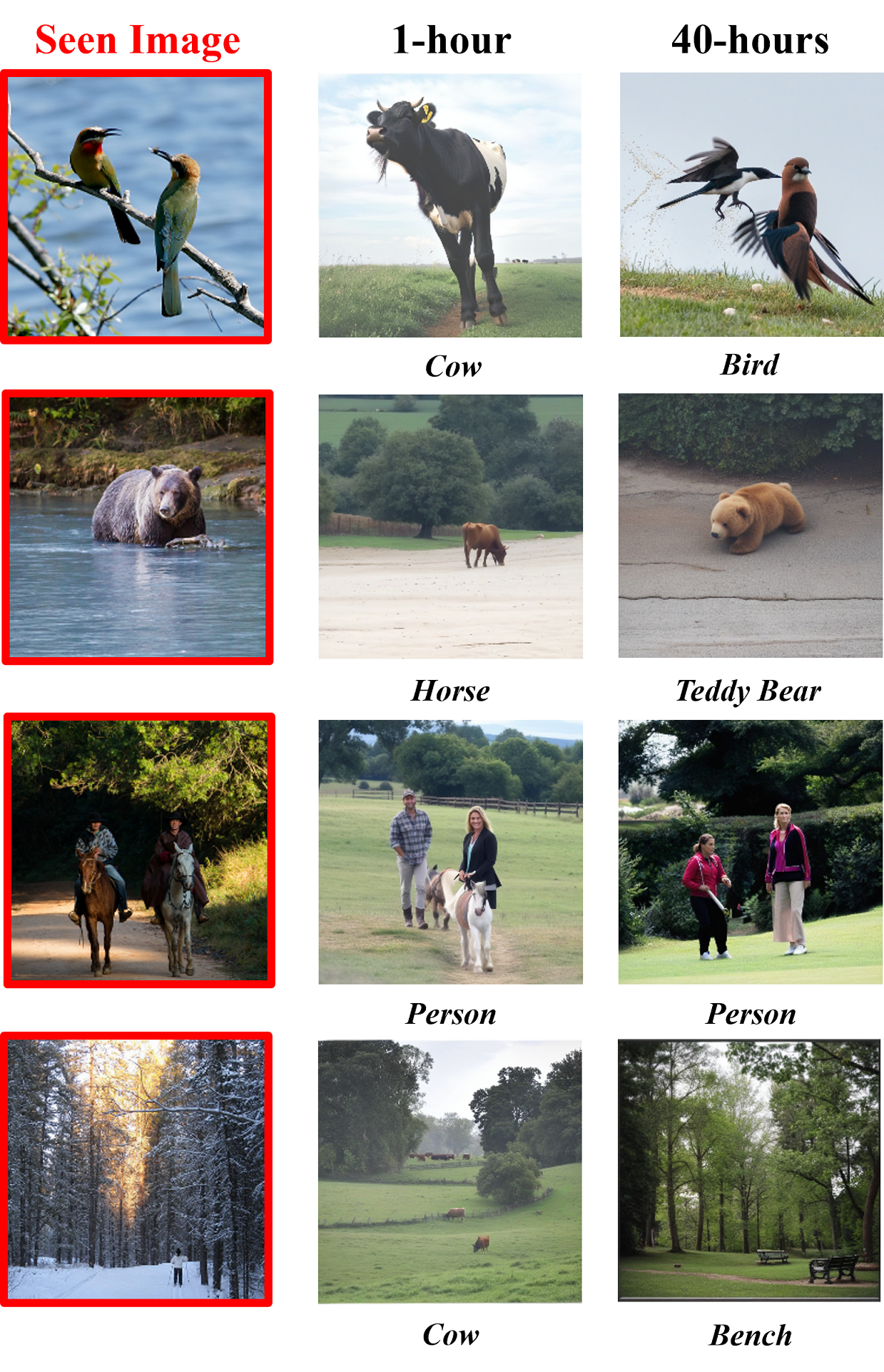
Figure 9. Failure Reconstructions.

The first reconstruction failures purely due to insufficient training data, e.g., the bear in the first line and the bird in the second line have bad semantics when only 1 hour of training data is available, but the semantics are progressively more accurate over 40 hours. The second type of reconstruction failure is caused by similar categories resulting in insufficient semantic accuracy, e.g., bears and teddy bears, cakes and pizzas, etc. The third type of reconstruction failure is due to the inability of category nouns to describe overly complex scenarios, especially when a person is present. Since MSCOCO’s category noun is only ’person’, it often appears that the person determines the categorization result while ignoring other objects, and the gender of the person is often not accurately generated. These are due to the fact that MindTuner only uses a single category noun, so more complex Pivot designs can be discussed in the future, whether for text generation or multi-classification.

Appendix C Additional Neuroscience Visualizations

In this section, we visualize the voxel weight maps of the other three subjects in Figure 13, 14 and 15, and the templates for the brain region references associated with nsdgeneral are shown in Figure 10. It can be seen that the content of the visual fingerprint is not quite the same across subjects, but both LoRA and SKip-LoRA have a portion of the primary visual cortex voxels that are significantly more heavily weighted than Ridge. As with Subj01, The visual fingerprint is more heavily weighted on the higher visual cortex for Subj02 and Subj05. However, this phenomenon was not observed for Subj07, which may be the reason why Subj07 performs worse on all the metrics. Further reasons need more explanations from neuroscientific mechanisms.

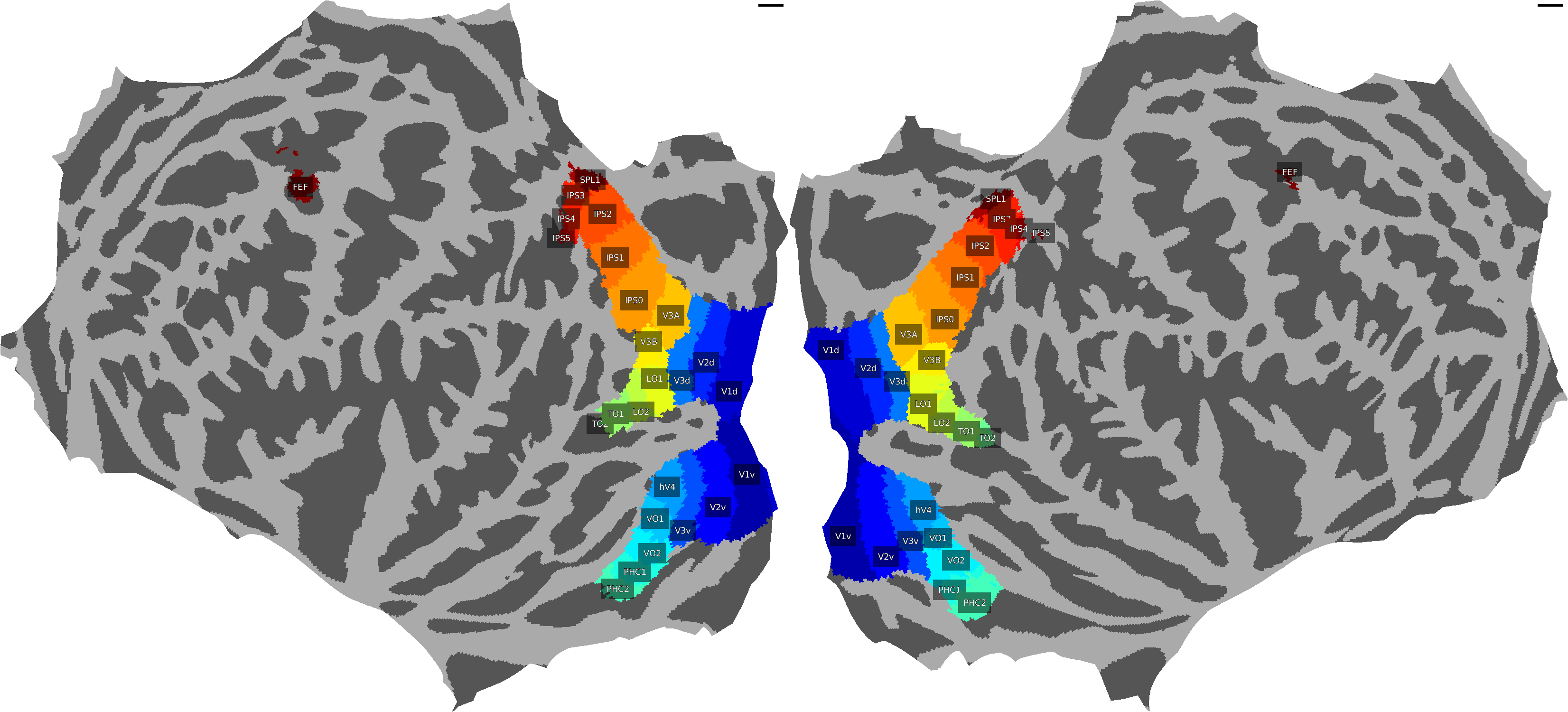
Figure 10. ROI reference map of visual cortex with template fsaverage.

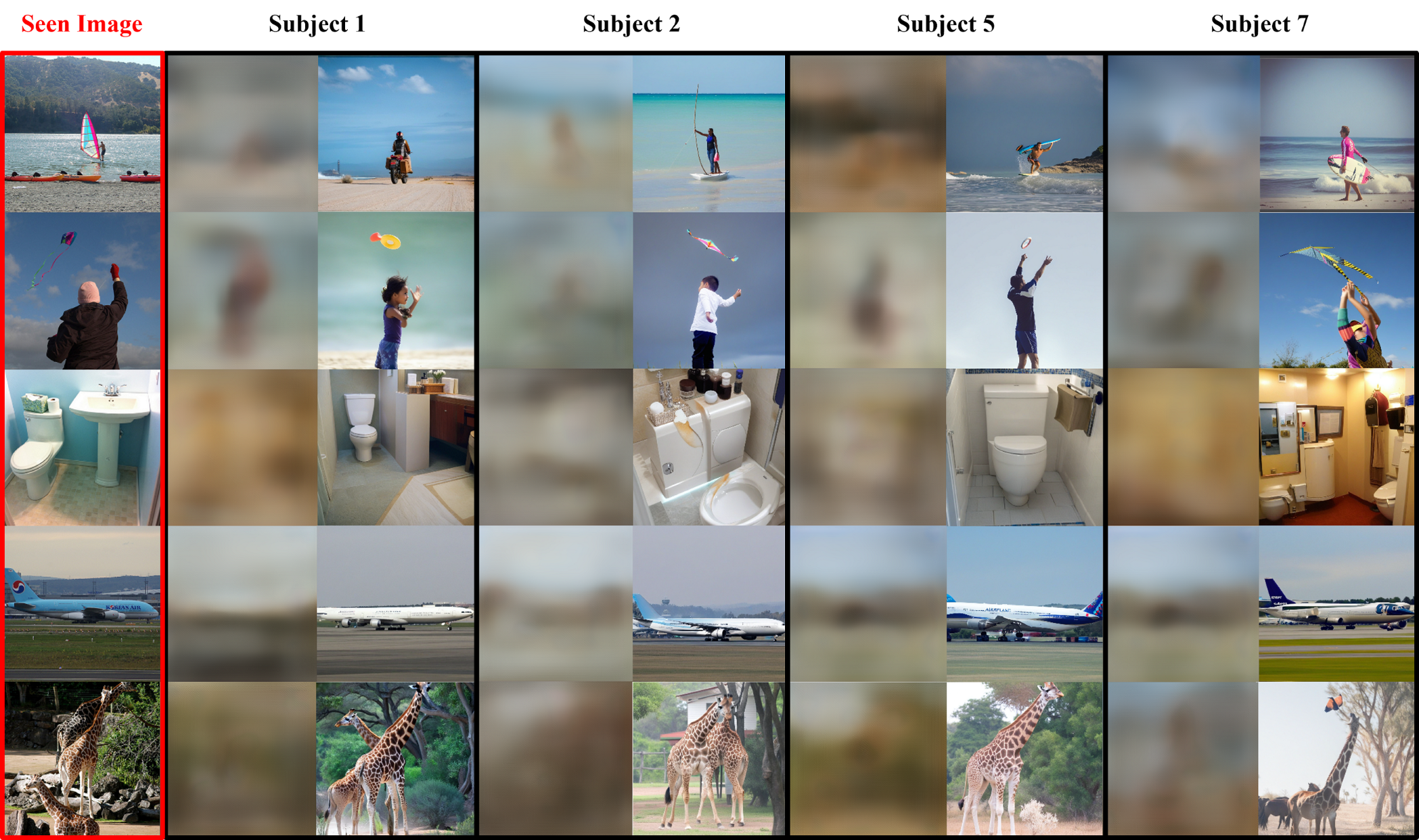
Figure 11. Subject’s specific visualizations of MindTuner with 1-hour training data.

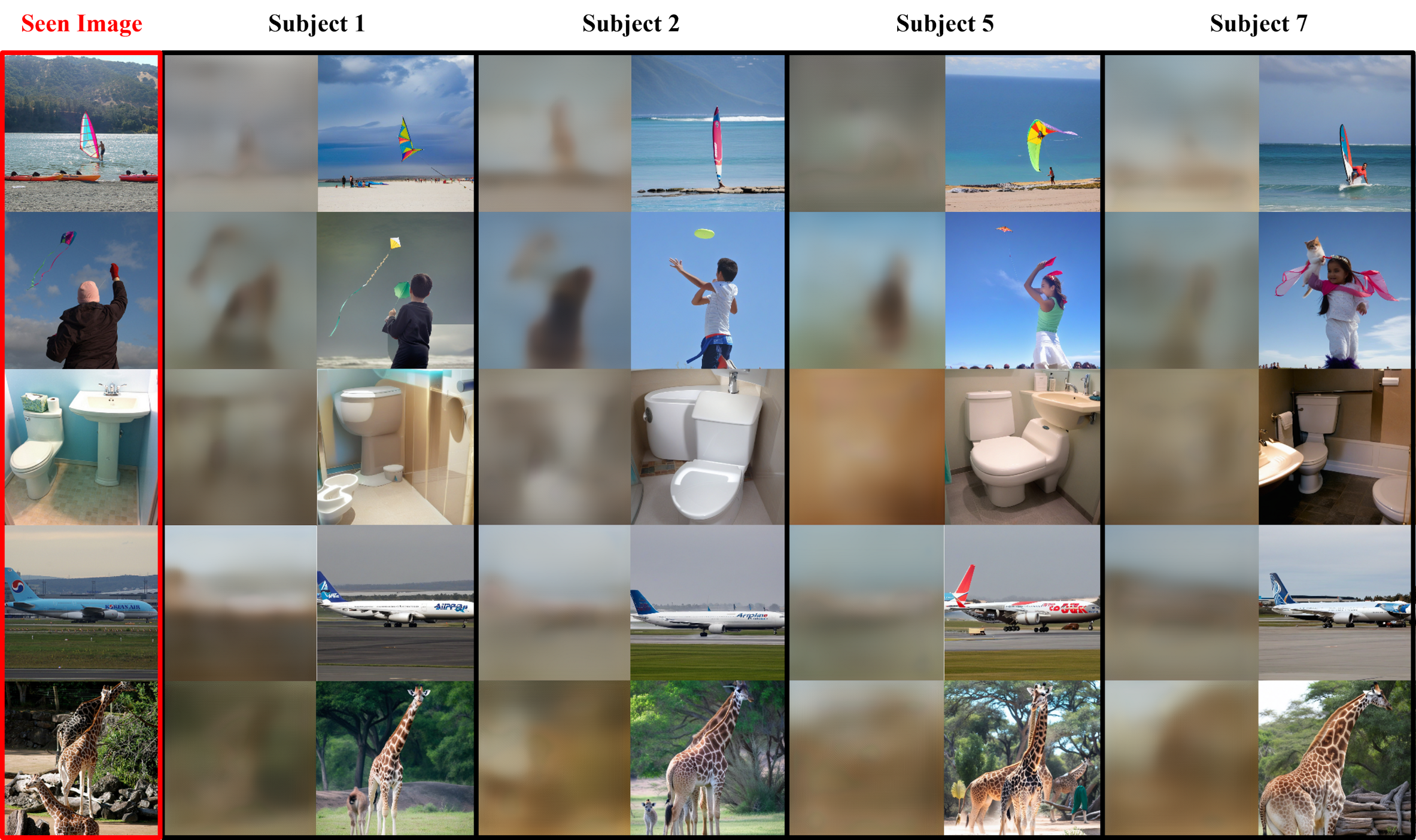
Figure 12. Subject’s specific visualizations of MindTuner with 40-hours training data.

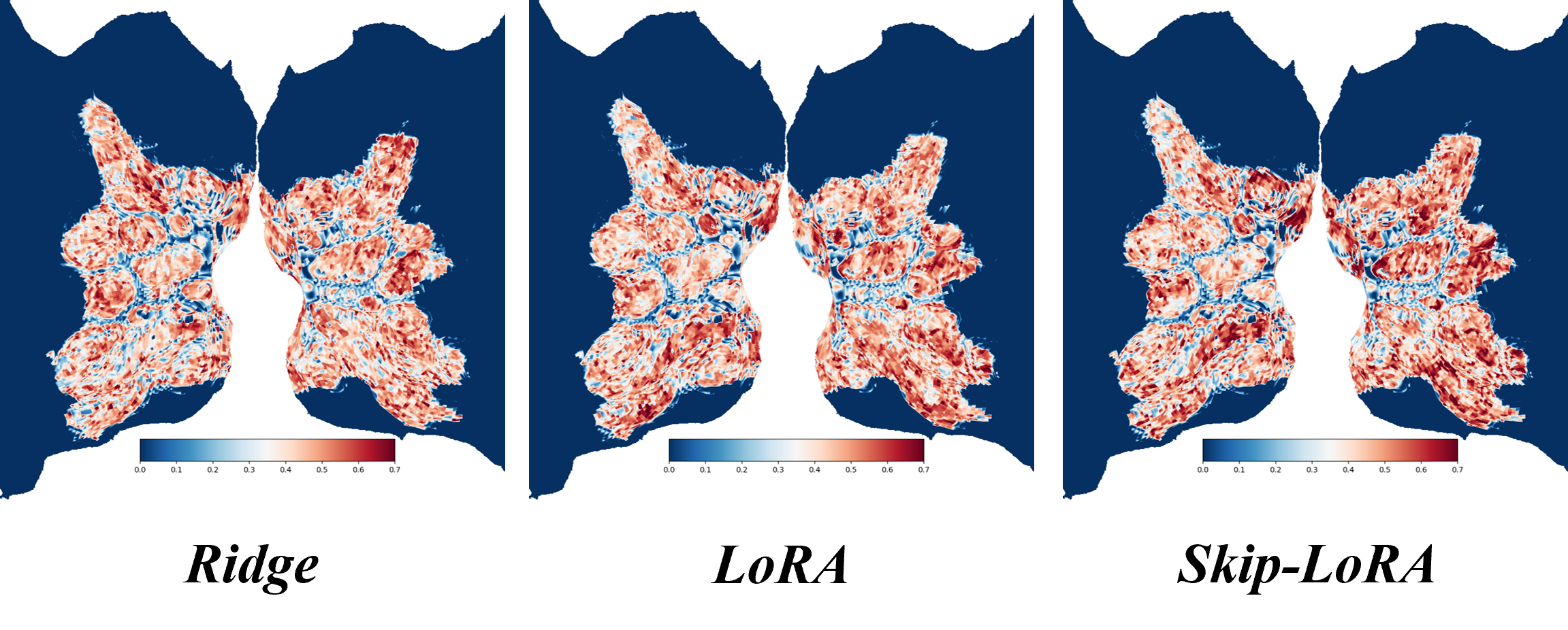
Figure 13. The importance of different ROIs of Subject 2 with fitted weights of the first layer.

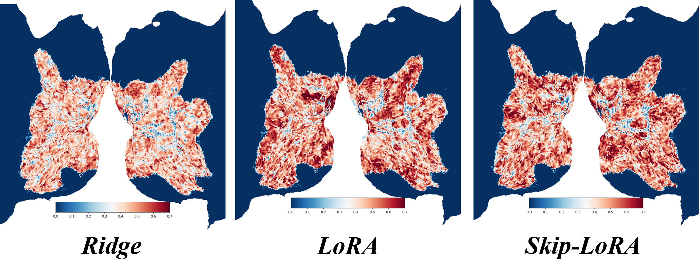
Figure 14. The importance of different ROIs of Subject 5 with fitted weights of the first layer.

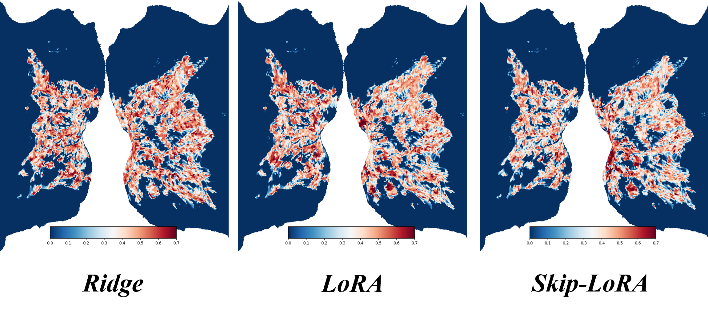
Figure 15. The importance of different ROIs of Subject 7 with fitted weights of the first layer.

References

- (1)
- Allen et al. (2022) Emily J Allen, Ghislain St-Yves, Yihan Wu, Jesse L Breedlove, Jacob S Prince, Logan T Dowdle, Matthias Nau, Brad Caron, Franco Pestilli, Ian Charest, et al. 2022. A massive 7T fMRI dataset to bridge cognitive neuroscience and artificial intelligence. Nature neuroscience 25, 1 (2022), 116–126.
- Bazeille et al. (2019) Thomas Bazeille, Hugo Richard, Hicham Janati, and Bertrand Thirion. 2019. Local optimal transport for functional brain template estimation. In Information Processing in Medical Imaging: 26th International Conference, IPMI 2019, Hong Kong, China, June 2–7, 2019, Proceedings 26. Springer, 237–248.
- Caron et al. (2020) Mathilde Caron, Ishan Misra, Julien Mairal, Priya Goyal, Piotr Bojanowski, and Armand Joulin. 2020. Unsupervised learning of visual features by contrasting cluster assignments. Advances in neural information processing systems 33 (2020), 9912–9924.
- Chen et al. (2017) Janice Chen, Yuan Chang Leong, Christopher J Honey, Chung H Yong, Kenneth A Norman, and Uri Hasson. 2017. Shared memories reveal shared structure in neural activity across individuals. Nature neuroscience 20, 1 (2017), 115–125.
- Chen et al. (2023) Zijiao Chen, Jiaxin Qing, Tiange Xiang, Wan Lin Yue, and Juan Helen Zhou. 2023. Seeing beyond the brain: Conditional diffusion model with sparse masked modeling for vision decoding. In Proceedings of the IEEE/CVF Conference on Computer Vision and Pattern Recognition. 22710–22720.
- Du et al. (2023) Changde Du, Kaicheng Fu, Jinpeng Li, and Huiguang He. 2023. Decoding visual neural representations by multimodal learning of brain-visual-linguistic features. IEEE Transactions on Pattern Analysis and Machine Intelligence (2023).
- Ferrante et al. (2023) Matteo Ferrante, Tommaso Boccato, and Nicola Toschi. 2023. Through their eyes: multi-subject Brain Decoding with simple alignment techniques. arXiv preprint arXiv:2309.00627 (2023).
- Fingelkurts et al. (2005) Andrew A Fingelkurts, Alexander A Fingelkurts, and Seppo Kähkönen. 2005. Functional connectivity in the brain—is it an elusive concept? Neuroscience & Biobehavioral Reviews 28, 8 (2005), 827–836.
- Gao et al. (2015) James S Gao, Alexander G Huth, Mark D Lescroart, and Jack L Gallant. 2015. Pycortex: an interactive surface visualizer for fMRI. Frontiers in neuroinformatics 9 (2015), 23.
- Horikawa and Kamitani (2017) Tomoyasu Horikawa and Yukiyasu Kamitani. 2017. Generic decoding of seen and imagined objects using hierarchical visual features. Nature communications 8, 1 (2017), 15037.
- Hu et al. (2021) Edward J Hu, Yelong Shen, Phillip Wallis, Zeyuan Allen-Zhu, Yuanzhi Li, Shean Wang, Lu Wang, and Weizhu Chen. 2021. Lora: Low-rank adaptation of large language models. arXiv preprint arXiv:2106.09685 (2021).
- Huang et al. (2022) Jessie Huang, Erica Busch, Tom Wallenstein, Michal Gerasimiuk, Andrew Benz, Guillaume Lajoie, Guy Wolf, Nicholas Turk-Browne, and Smita Krishnaswamy. 2022. Learning shared neural manifolds from multi-subject FMRI data. In 2022 IEEE 32nd International Workshop on Machine Learning for Signal Processing (MLSP). IEEE, 01–06.
- Kim et al. (2020) Sungnyun Kim, Gihun Lee, Sangmin Bae, and Se-Young Yun. 2020. Mixco: Mix-up contrastive learning for visual representation. arXiv preprint arXiv:2010.06300 (2020).
- Kneeland et al. (2023) Reese Kneeland, Jordyn Ojeda, Ghislain St-Yves, and Thomas Naselaris. 2023. Brain-optimized inference improves reconstructions of fMRI brain activity. arXiv preprint arXiv:2312.07705 (2023).
- Lin et al. (2022) Sikun Lin, Thomas Sprague, and Ambuj K Singh. 2022. Mind reader: Reconstructing complex images from brain activities. Advances in Neural Information Processing Systems 35 (2022), 29624–29636.
- Linden (2021) David Linden. 2021. Section 3 - Introduction. In fMRI Neurofeedback, Michelle Hampson (Ed.). Academic Press, 161–169. https://doi.org/10.1016/B978-0-12-822421-2.00008-9
- Loshchilov and Hutter (2017) Ilya Loshchilov and Frank Hutter. 2017. Decoupled weight decay regularization. arXiv preprint arXiv:1711.05101 (2017).
- Lu et al. (2023) Yizhuo Lu, Changde Du, Qiongyi Zhou, Dianpeng Wang, and Huiguang He. 2023. MindDiffuser: Controlled Image Reconstruction from Human Brain Activity with Semantic and Structural Diffusion. In Proceedings of the 31st ACM International Conference on Multimedia. 5899–5908.
- Mai and Zhang (2023) Weijian Mai and Zhijun Zhang. 2023. Unibrain: Unify image reconstruction and captioning all in one diffusion model from human brain activity. arXiv preprint arXiv:2308.07428 (2023).
- Mou et al. (2024) Chong Mou, Xintao Wang, Liangbin Xie, Yanze Wu, Jian Zhang, Zhongang Qi, and Ying Shan. 2024. T2i-adapter: Learning adapters to dig out more controllable ability for text-to-image diffusion models. In Proceedings of the AAAI Conference on Artificial Intelligence, Vol. 38. 4296–4304.
- Nie et al. (2023) Xixi Nie, Bo Hu, Xinbo Gao, Leida Li, Xiaodan Zhang, and Bin Xiao. 2023. BMI-Net: A Brain-inspired Multimodal Interaction Network for Image Aesthetic Assessment. In Proceedings of the 31st ACM International Conference on Multimedia (, Ottawa ON, Canada,) (MM ’23). Association for Computing Machinery, New York, NY, USA, 5514–5522. https://doi.org/10.1145/3581783.3611996
- Ozcelik and VanRullen (2023) Furkan Ozcelik and Rufin VanRullen. 2023. Brain-diffuser: Natural scene reconstruction from fmri signals using generative latent diffusion. arXiv preprint arXiv:2303.05334 (2023).
- Qian et al. (2023) Xuelin Qian, Yun Wang, Jingyang Huo, Jianfeng Feng, and Yanwei Fu. 2023. fmri-pte: A large-scale fmri pretrained transformer encoder for multi-subject brain activity decoding. arXiv preprint arXiv:2311.00342 (2023).
- Radford et al. (2021) Alec Radford, Jong Wook Kim, Chris Hallacy, Aditya Ramesh, Gabriel Goh, Sandhini Agarwal, Girish Sastry, Amanda Askell, Pamela Mishkin, Jack Clark, et al. 2021. Learning transferable visual models from natural language supervision. In International conference on machine learning. PMLR, 8748–8763.
- Ramesh et al. (2022) Aditya Ramesh, Prafulla Dhariwal, Alex Nichol, Casey Chu, and Mark Chen. 2022. Hierarchical text-conditional image generation with clip latents. arXiv preprint arXiv:2204.06125 (2022).
- Rombach et al. (2022) Robin Rombach, Andreas Blattmann, Dominik Lorenz, Patrick Esser, and Björn Ommer. 2022. High-resolution image synthesis with latent diffusion models. In Proceedings of the IEEE/CVF conference on computer vision and pattern recognition. 10684–10695.
- Scotti et al. (2023) Paul S Scotti, Atmadeep Banerjee, Jimmie Goode, Stepan Shabalin, Alex Nguyen, Ethan Cohen, Aidan J Dempster, Nathalie Verlinde, Elad Yundler, David Weisberg, et al. 2023. Reconstructing the Mind’s Eye: fMRI-to-Image with Contrastive Learning and Diffusion Priors. arXiv preprint arXiv:2305.18274 (2023).
- Scotti et al. (2024) Paul S Scotti, Mihir Tripathy, Cesar Kadir Torrico Villanueva, Reese Kneeland, Tong Chen, Ashutosh Narang, Charan Santhirasegaran, Jonathan Xu, Thomas Naselaris, Kenneth A Norman, et al. 2024. MindEye2: Shared-Subject Models Enable fMRI-To-Image With 1 Hour of Data. arXiv preprint arXiv:2403.11207 (2024).
- Shen et al. (2019) Guohua Shen, Tomoyasu Horikawa, Kei Majima, and Yukiyasu Kamitani. 2019. Deep image reconstruction from human brain activity. PLoS computational biology 15, 1 (2019), e1006633.
- Smith and Topin (2019) Leslie N Smith and Nicholay Topin. 2019. Super-convergence: Very fast training of neural networks using large learning rates. In Artificial intelligence and machine learning for multi-domain operations applications, Vol. 11006. SPIE, 369–386.
- St-Yves et al. (2022) Ghislain St-Yves, Emily J Allen, Yihan Wu, Kendrick Kay, and Thomas Naselaris. 2022. Brain-optimized neural networks learn non-hierarchical models of representation in human visual cortex. bioRxiv (2022), 2022–01.
- Stringer et al. (2019) Carsen Stringer, Marius Pachitariu, Nicholas Steinmetz, Matteo Carandini, and Kenneth D Harris. 2019. High-dimensional geometry of population responses in visual cortex. Nature 571, 7765 (2019), 361–365.
- Takagi and Nishimoto (2023) Yu Takagi and Shinji Nishimoto. 2023. High-resolution image reconstruction with latent diffusion models from human brain activity. In Proceedings of the IEEE/CVF Conference on Computer Vision and Pattern Recognition. 14453–14463.
- Tan and Quoc ([n. d.]) Mingxing Tan and V Le Quoc. [n. d.]. EfficientNet: Rethinking Model Scaling for Convolutional Neural Networks, September 2020. arXiv preprint arXiv:1905.11946 ([n. d.]).
- Thual et al. (2023) Alexis Thual, Yohann Benchetrit, Felix Geilert, Jérémy Rapin, Iurii Makarov, Hubert Banville, and Jean-Rémi King. 2023. Aligning brain functions boosts the decoding of visual semantics in novel subjects. arXiv preprint arXiv:2312.06467 (2023).
- Wang et al. (2009) Jun Wang, Eric Pohlmeyer, Barbara Hanna, Yu-Gang Jiang, Paul Sajda, and Shih-Fu Chang. 2009. Brain state decoding for rapid image retrieval. In Proceedings of the 17th ACM International Conference on Multimedia (Beijing, China) (MM ’09). Association for Computing Machinery, New York, NY, USA, 945–954. https://doi.org/10.1145/1631272.1631463
- Wang et al. (2022) Jianfeng Wang, Zhengyuan Yang, Xiaowei Hu, Linjie Li, Kevin Lin, Zhe Gan, Zicheng Liu, Ce Liu, and Lijuan Wang. 2022. Git: A generative image-to-text transformer for vision and language. arXiv preprint arXiv:2205.14100 (2022).
- Wang et al. (2004) Zhou Wang, Alan C Bovik, Hamid R Sheikh, and Eero P Simoncelli. 2004. Image quality assessment: from error visibility to structural similarity. IEEE transactions on image processing 13, 4 (2004), 600–612.
- Wang et al. (2020) Zixuan Wang, Yuki Murai, and David Whitney. 2020. Idiosyncratic perception: a link between acuity, perceived position and apparent size. Proceedings of the Royal Society B 287, 1930 (2020), 20200825.
- Xia et al. (2024) Weihao Xia, Raoul de Charette, Cengiz Oztireli, and Jing-Hao Xue. 2024. Dream: Visual decoding from reversing human visual system. In Proceedings of the IEEE/CVF Winter Conference on Applications of Computer Vision. 8226–8235.
- Zhang et al. (2023) Lvmin Zhang, Anyi Rao, and Maneesh Agrawala. 2023. Adding conditional control to text-to-image diffusion models. In Proceedings of the IEEE/CVF International Conference on Computer Vision. 3836–3847.
- Zhao et al. (2014) Shijie Zhao, Xi Jiang, Junwei Han, Xintao Hu, Dajiang Zhu, Jinglei Lv, Tuo Zhang, Lei Guo, and Tianming Liu. 2014. Decoding Auditory Saliency from FMRI Brain Imaging. In Proceedings of the 22nd ACM International Conference on Multimedia (Orlando, Florida, USA) (MM ’14). Association for Computing Machinery, New York, NY, USA, 873–876. https://doi.org/10.1145/2647868.2655039