Spreading Code Optimization for Low-Earth Orbit Satellites via Mixed-Integer Convex Programming

Abstract

Optimizing the correlation properties of spreading codes is critical for minimizing inter-channel interference in satellite navigation systems. By improving the codes’ correlation sidelobes, we can enhance navigation performance while minimizing the required spreading code lengths. In the case of low earth orbit (LEO) satellite navigation, shorter code lengths (on the order of a hundred) are preferred due to their ability to achieve fast signal acquisition. Additionally, the relatively high signal-to-noise ratio (SNR) in LEO systems reduces the need for longer spreading codes to mitigate inter-channel interference. In this work, we propose a two-stage block coordinate descent (BCD) method which optimizes the codes’ correlation properties while enforcing the autocorrelation sidelobe zero (ACZ) property. In each iteration of the BCD method, we solve a mixed-integer convex program (MICP) over a block of 25 binary variables. Our method is applicable to spreading code families of arbitrary sizes and lengths, and we demonstrate its effectiveness for a problem with 66 length-127 codes and a problem with 130 length-257 codes.

1 Introduction

In this work, we consider the design of navigation spreading codes for future low-Earth orbit (LEO) satellite constellations. LEO constellations are typically comprised of hundreds, or even thousands, of low-cost satellites [1]. Commercial examples include Iridium [2], OneWeb [3], and the constellations proposed by Samsung [4], SpaceX [5], and Xona [6]. Several of those constellations are primarily designed to deliver global internet coverage, but can also be leveraged for navigation [7]. In addition, the European space agency (ESA) recently announced the LEO-PNT program, which will test capabilities for navigation and timing using LEO satellites [8]. See the review [9] for a survey of recent developments in LEO PNT.

All code-division multiple access (CDMA) systems, including satellite navigation systems, rely on spreading codes [10]. In CDMA, each satellite modulates its signal with a unique and known spreading code, which is typically a binary sequence. The receiver then correlates the received signal with replicas of each satellite’s spreading code to identify the source of the transmitted signal. Therefore, it is necessary for the spreading codes to have low pairwise cross-correlation to minimize inter-channel interference. Additionally, it is important for the codes to have low autocorrelation sidelobes to minimize the effects of multi-path and self-interference, and to ensure that the time of signal reception can be correctly determined.

LEO systems suffer less path loss than navigation systems in medium-Earth orbit (MEO) such as GPS, improving signal strength 1000-fold, or by 30dbB [1]. Therefore, short code lengths (on the order of a hundred) may be preferable since short code lengths correspond to fast signal acquisition, and the relatively high signal-to-noise ratio (SNR) means that long spreading codes are not needed for low inter-channel interference [11].

In this work, we propose a two-stage block coordinate descent (BCD) method for finding good spreading codes satisfying the autocorrelation sidelobe zero (ACZ) property [12, 13]. The ACZ property requires that the shift-one autocorrelation of each code is minimal. Imposing the ACZ constraint is useful for ensuring that the tracking performance is consistently good across all the satellites in the constellation. [13, 12]. The first stage of our BCD method finds a feasible code family that satisfies the ACZ property, and the second stage minimizes the sum of squared auto- and cross-correlation sidelobes, without breaking the ACZ property.

Our method is based on the recently-proposed mixed-integer convex program (MICP) approach to spreading code optimization [14, 15, 16], which has shown promising results for optimizing spreading codes for MEO applications. In that approach, the spreading code optimization problem is formulated as a mixed-integer convex program (MICP). In each iteration of BCD, we solve the optimization problem exactly over a subset of the binary variables, with the others held fixed. The partial minimization problem is also an MICP, and may be solved using an MICP solver such as Gurobi [17]. In this work, we handle the ACZ constraint by using the fact that it may be enforced using linear inequality constraints [16].

Unlike the prior works [15, 16], we focus on the LEO setting, where the number of codes is relatively large. In this regime, the choice of the subset of binary variables to optimize over in each iteration of BCD is an important consideration. We propose a variable subset selection strategy that can achieve a small per-iteration runtime cost by tuning the number of codes from which the binary variables are selected in a given iteration. For a fixed variable subset size, choosing the variables from a small number of codes can make the subproblems more difficult to solve, and can lead large per-iteration runtime cost. On the other hand, choosing the variables from a large number of codes can make the subproblems easier to solve, but can still lead to a large per-iteration runtime cost due to the computational overhead from setting up the MICP subproblems.

The rest of the paper is organized as follows. We review related work in Subsection 1.1. In Section 2, we describe the spreading code optimization problem and the MICP formulation of the problem. In Section 3, we describe the proposed BCD. Section 4 presents numerical results, and Section 5 concludes.

1.1 Related work

The problem of designing spreading codes with good correlation properties has a long history. Current satellite navigation systems, such as GPS, use pseudo-random noise (PRN) codes such as Gold codes [18], which can be generated using linear-feedback shift registers, and the Weil codes [19, 20], which are based on Legendre sequences. While those codes satisfy provable bounds on their auto- and cross-correlation, they are only available for specific lengths and number of codes, and cannot be easily modified. For example, truncating or extending those codes by even a single bit can compromise their correlation properties [12].

To address those limitations, there has been growing interest in designing the spreading codes by directly optimizing the auto- and cross-correlation. Population-based methods, such as genetic algorithms [21, 22], natural evolution strategies [23], and the cross-entropy method [24] have been applied, and the European Union’s Galileo constellation uses spreading codes designed by a genetic algorithm [12, 25]. However, those methods do not consider the structure in the objective, and often require extensive tuning in order to work well. In addition, they have focused on codes for medium-Earth orbit (MEO) constellations such as GPS [23, 16] and Galileo constellations [12, 25]. In those settings, the code length is orders of magnitude larger than the number of the codes; this is neccessary for good system performance due to the relatively lower SNR in the MEO setting.

Coordinate descent and BCD methods have been proposed to optimize sets of binary sequences for multiple-input multiple-output (MIMO) radar systems [26, 27, 28, 29, 15]. Like the spreading codes for navigation systems, the binary sequences used in those applications are required to have low auto- and cross-correlation. However, the aforementioned works only optimize over either a single binary variable at a time, or a small number (e.g., four), using an exhaustive search. In contrast, by using branch and bound to perform the BCD updates [30, 15, 16], we can efficiently optimize over large blocks of binary variables, e.g., $25$, during each BCD iteration. This approach is particularly effective for designing LEO satellite spreading codes due to the relatively small code lengths and large family sizes.

Finally, penalty methods [31] and semidefinite relaxations [32] have been proposed to design sets of complex-valued, continuous-phase sequences with constant magnitude. However, we focus on binary sequences, since they are often preferred in practice due to ease of implementation. Moreover, the discretization of continuous sequences has been found to give poor performance [26, 27].

Other methods construct new sequences and sequence sets by combining pre-existing binary sequences with desirable correlation properties, such as Gold codes or optimized sequence sets [33, 34].

2 Spreading code optimization

2.1 Preliminaries

A spreading code family is a set of $m$ binary code sequences, each of length $n$. We refer to the code family as $X=(x^{0},\ldots,x^{m-1})$, where $x^{i}\in\{\pm 1\}^{n}$ is the $i$th code in the family. The code family may be represented as a binary matrix $X\in\{\pm 1\}^{n\times m}$, where $x^{i}$ is the $i$th column of $X$.

Cross-correlation.

The cross-correlation between two binary codes $w,v\in\{\pm 1\}^{n}$ is a vector $(w\star v)\in{\mathbb{R}}^{n}$, where

$$(w\star v)_{k}=\sum_{s=0}^{n-1}w_{s}v_{(s+k)_{\bmod n}},\quad k=0,\ldots,n-1.$$ (1)

That is, $(w\star v)_{k}$ is the inner product between $w$ and a $k$-circularly shifted version of $v$. The cross-correlation may also defined for negative-valued shifts, noting that

$$(w\star v)_{-k}=(w\star v)_{k-n},\quad k=0,\ldots,n-1.$$

Autocorrelation.

We refer to the cross-correlation of a binary sequence $w\in\{\pm 1\}^{n}$ with itself as the autocorrelation of $w$. Note that the shift-zero autocorrelation is given by $(w\star w)_{0}=\|w\|_{2}^{2}=n$, regardless of the value of $w$. By symmetry, $(w\star w)_{k}=(w\star w)_{-k}$, for all $k=0,\ldots,n-1$.

Autocorrelation sidelobe zero (ACZ).

A binary sequence $w\in\{\pm 1\}^{n}$ satisfies the ACZ property if its shift-one autocorrelation $(w\star w)_{1}$ is minimal. For even-valued $n$, this corresponds to the requirement that $(w\star w)_{1}=0$. For odd-valued $n$, the autocorrelation cannot be zero, and so we instead require that $|(w\star w)_{1}|=1$. If the measured correlation at shifts zero and one are too similar, the receiver may erroneously lose the signal lock. The ACZ property ensures that the difference between the shift-zero peak and shift-one autocorrelation is large for all of the codes in the family. This can improve the consistency in ranging performance across the code family, especially when the code lengths are short. Indeed, it has been shown that maximizing the difference between the shift-zero peak and the shift-one autocorrelation minimizes the Cramer-Rao lower bound for the ranging estimation problem [35, 36]. The ACZ property has also been applied in practice; the Galileo constellation uses even-length spreading codes which were designed to satisfy the ACZ property [13, 12]. In this work, we formulate the ACZ property as a set of linear inequality or equality constraints. Therefore, the ACZ property may be readily incorporated into the MICP formulation of the spreading code optimization problem, as we discuss in the following subsection.

2.2 Spreading code optimization problem

An ideal sequence set $X=(x^{0},\ldots,x^{m-1})$ has $(x^{i}\star x^{j})_{k}$ close to zero for all pairs of sequences $x^{i}$ and $x^{j}$ and at all shifts $k=0,\ldots,n-1$. In this work, we minimize the sum of squared auto- and cross-correlation magnitudes, subject to constraint that the autocorrelation sidelobe zero (ACZ) property is satisfied.

The spreading code optimization problem may be written as

minimize $$\sum_{i=0}^{m-1}\sum_{j=i}^{m-1}\sum_{k=0}^{n-1}\left(x^{i}\star x^{j}\right)_{k}^{2}$$ (2a)

subject to $$\left|(x^{i}\star x^{i})_{1}\right|\leq g, i=0,\ldots,m-1,$$ (2b)

$$x^{i}\in\{\pm 1\}^{n}, i=0,\ldots,m-1.$$ (2c)

Here, $g$ is a parameter that takes value $0$ if $n$ is even, and $1$ if $n$ is odd. In some contexts, the sum of squares objective is referred to as the integrated sidelobe level (ISL) [37, 26]. For ease of notation, we do not exclude the zero-shift autocorrelation terms from the objective. Since those terms are constant-valued, they do not affect the solution of the optimization problem.

Note that the objective function (2a) is a non-convex quartic function of the variables, since each term $\left(x^{i}\star x^{j}\right)_{k}$ is a nonconvex quadratic function of the binary variables. Similarly, the ACZ constraint (2b) is a nonconvex constraint. The nonconvex objective and constraints, combined with the nonconvex binary constraints, make the problem (2a)–(2c) a challenging combinatorial optimization problem. In subsection 2.3, we discuss how the problem may be reformulated as a MICP and how the resulting convex structure may be exploited [15, 16].

2.3 MICP formulation

The cross-correlation function (1) involxves a sum of products of binary variables. By representing each product using a new auxiliary variable, the cross-correlation becomes a sum of auxiliary variables, and the objective function (2a) may be written as a convex quadratic function of the auxiliary variables.

Binary variable product.

This approach is made possible by the following fact, which may be verified using a truth table [38]. Suppose that $a,b\in\{\pm 1\}$ and $c\in{\mathbb{R}}$. Then, $c=ab$ if and only if

$$c \leq b-a+1,$$

$$c \leq a-b+1,$$

$$c \geq-a-b-1,$$

$$c \geq a+b-1.$$

We refer to the above constraints as linking constraints, since they couple the binary variables $a$ and $b$ to the auxiliary variable $c$ that represents their product.

Spreading code optimization as a MICP.

Using the aforementioned representation of binary variable products, we may represent the spreading code optimization problem (2) as a MICP. Let $\{z^{i,j}_{s,l}\}$ be a set of auxiliary variables such that $z^{i,j}_{s,l}$ represents the product $x^{i}_{s}x^{j}_{l}$, for each $i,j=0,\ldots,m-1$ and $s,l=0,\ldots,n-1$. Then, the cross-correlation between codes $x^{i}$ and $x^{j}$ may be written as a sum of the auxiliary variables, given by

$$(x^{i}\star x^{j})_{k}=\sum_{s=0}^{n-1}x^{i}_{s}x^{j}_{(s+k)_{\bmod n}}=\sum_{s=0}^{n-1}z^{i,j}_{s,(s+k)_{\bmod n}},\quad k=0,\ldots,n-1.$$

Here, each auxiliary variable $z^{i,j}_{s,k}$ satisfies a set of linking constraints that couple it to the binary variables $x^{i}_{s}$ and $x^{j}_{k}$. The spreading code optimization problem (2a) – (2c) may therefore be written as

minimize $$\sum_{i=0}^{m-1}\sum_{j=i}^{m-1}\sum_{k=0}^{n-1}\left(\sum_{s=0}^{n-1}z_{s,(s+k)_{\bmod n}}^{i,j}\right)^{2}$$ (3a)

subject to $$-g\leq\sum_{s=0}^{n-1}z_{s,(s+1)_{\bmod n}}^{i,i}\leq g, i=0,\ldots,m-1,$$ (3b)

$$x^{i}\in\{\pm 1\}^{n\times m}, i=0,\ldots,m-1,$$ (3c)

$$z_{s,l}^{i,j}\leq x_{l}^{j}-x_{s}^{i}+1,$$ (3d)

$$z_{s,l}^{i,j}\leq x_{s}^{i}-x_{l}^{j}+1,$$ (3e)

$$z_{s,l}^{i,j}\geq-x_{l}^{j}-x_{s}^{i}-1,$$ (3f)

$$z_{s,l}^{i,j}\geq x_{s}^{i}+x_{l}^{j}-1,$$ (3g)

$$i,j=0,\ldots,m-1,\,\,s,l=0,\ldots,n-1.$$

Here, the linear equality constraints (3b) enforces the ACZ property and the linking constraints (3d) – (3g) couple the binary variables to the auxiliary variables. Since the optimization problem (3) involves minimizing a convex quadratic function subject to binary, linear inequality, and linear equality constraints, it is a MICP [14]. More specifically, it is a mixed-integer quadratic program, since it becomes a quadratic program when the binary constraints (3c) are relaxed.

Number of auxiliary variables.

A total of ${nm\choose 2}$ additional auxiliary variables, along with $4{nm\choose 2}$ linking constraints, are required to transform (2) into the MICP (3). Therefore, the problem size, in terms of the number of additional auxiliary variables and constraints, grows quadratically with $nm$. This may be prohibitive for relevant values of $nm$, which may be in the tens of thousands. In Section 2.4, we show how the problem may be simplified when we are only interested in optimizing over only a subset of $B$ of the the binary variables, with the others held fixed. In that case, the number of auxiliary variables and constraints grows on the order of $O(B^{2})$, rather than $O(n^{2}m^{2})$.

2.4 Partial minimization

In this subsection, we describe the partial minimization of (3) over a subset of the binary variables. Note that since (3) is an MICP, any partial minimization problem derived from (3) is also an MICP. The partial minimization problem is useful for the block coordinate descent algorithm discussed in Section 3.1.

Suppose we wish to optimize only over a variable index set

$$S\subseteq\left\{(i,r)\mid 0\leq i\leq m-1,\quad 0\leq r\leq n-1\right\}.$$ (4)

Each index $(i,r)\in S$ corresponds to the binary variable $x_{r}^{i}$, which is the $r$th element of the $i$th code sequence. The variables not indexed by $S$ are held fixed. That is, we wish to solve the MICP (3) with the additional equality constraints

$$x^{i}_{r}=\tilde{x}^{i}_{r},\quad(i,r)\not\in S,$$

for some fixed values $\tilde{x}^{i}_{r}\in\{\pm 1\}$, for all $(i,r)\not\in S$.

Since it is only necessary to include auxiliary variables to represent products between binary variables that appear in $S$, the partial minimization MICP may be simplified in this case.

In the partial minimization problem, the cross-correlation between any two codes $x^{i}$ and $x^{j}$ may be expressed as an affine function of the auxiliary and binary variables, with coefficients that depend on the values of the fixed binary variables. That is, we may write the cross-correlation between two codes $x^{i}$ and $x^{j}$ as

$$(x^{i}\star x^{j})_{k}=\sum_{s=0}^{n-1}y^{i,j}_{s,k},\quad k=0,\ldots,n-1,$$

where

$$y^{i,j}_{s,k}\vcentcolon=\begin{cases}z^{i,j}_{s,(s+k)_{\bmod n}}&\textrm{if $(i,s)\in S$ and $(j,(s+k)_{\bmod n})\in S$},\\ x^{i}_{s}\tilde{x}^{j}_{(s+k)_{\bmod n}}&\textrm{if $(i,s)\in S\,\,\textrm{and}\,\,(j,(s+k)_{\bmod n}),\,(j,(s-k)_{\bmod n})\not\in S$},\\ \tilde{x}^{i}_{s}\tilde{x}^{j}_{(s+k)_{\bmod n}}&\textrm{otherwise.}\end{cases}$$ (5)

There are three cases: both $x^{i}_{s}$ and $x^{j}_{(s+k)_{\bmod n}}$ are variables in the partial minimization, only one of them is a variable, or neither of them is a variable.

Since the cross-correlation may be represented using an affine function of the auxiliary and binary variables, the objective function (3a) remains convex quadratic. Here, only ${|S|\choose 2}$ auxiliary variables are required, since we only need to represent products between binary variables indexed by $S$.

Let $C_{S}$ be the set of columns, or code sequences, that contain at least one binary variable indexed by $S$. That is,

$$C_{S}=\left\{i\mid(i,s)\in S\right\}.$$ (6)

The number of terms in the objective function (3a) may be reduced to the auto- and cross-correlation terms between codes in $C_{S}$. That is, the partial minimization problem may be written as the MICP

minimize $$\sum_{i\in C_{S}}\sum_{\begin{subarray}{c}j=0\\ j\neq C_{S}\,\,\textrm{or}\,\,j\geq i\end{subarray}}^{m-1}\sum_{k=0}^{n-1}\left(\sum_{s=0}^{n-1}y_{s,k}^{i,j}\right)^{2}$$ (7a)

subject to $$-g\leq\sum_{s=0}^{n-1}z_{s,(s+1)_{\bmod n}}^{i,i}\leq g,\ i=0,\ldots,m-1,$$ (7b)

$$x^{i}_{s}\in\{\pm 1\}, (i,s)\in S,$$ (7c)

$$z_{s,l}^{i,j}\leq x_{l}^{j}-x_{s}^{i}+1,$$ (7d)

$$z_{s,l}^{i,j}\leq x_{s}^{i}-x_{l}^{j}+1,$$ (7e)

$$z_{s,l}^{i,j}\geq-x_{l}^{j}-x_{s}^{i}-1,$$ (7f)

$$z_{s,l}^{i,j}\geq x_{s}^{i}+x_{l}^{j}-1,$$ (7g)

$$(i,s),(j,l)\in S\times S,$$

where $y^{i,j}_{s,k}$ are given by (5), and $g$ is a constant that is either $0$ if $n$ is even, or $1$ if $n$ is odd.

3 Block coordinate descent

In this section, we describe a block coordinate descent (BCD) method for finding a good solution to the spreading code optimization problem (3). In our approach, we iteratively solve the partial minimization problem (7) over a block, or subset of the binary variables, with the others held fixed [27, 30, 15, 16]. The partial minimization problems are solved exactly using an MICP solver, such as Gurobi [17] or SCIP [39]. The BCD method is described in Subsection 3.1, and variable subset selection strategies are discussed in Subsection 3.2.

3.1 Method

BCD is a particularly compelling method for handling the MICP (3), since the MICP is difficult to solve directly, but its partial minimization (7) can be solved effectively in practice.

Basic BCD method.

The basic BCD method proceeds starting from an initial code family $X^{0}\in\{\pm 1\}^{n\times m}$. In the $k$th iteration, we compute the next code family $X^{k+1}$ by performing the following steps:

1. Select a variable subset $S^{k}\subseteq\left\{(i,r)\mid 0\leq i\leq m-1,\,0\leq r\leq n-1\right\}$.

2. Solve the partial minimization problem (7) over $S^{k}$, with the other binary variables fixed to their previous values in $X^{k}$.

3. Set $X^{k+1}$ to be the solution to the partial minimization problem.

BCD is a descent method, i.e., the objective value is nonincreasing, since the block update steps are solved to optimality. We discuss strategies for selecting the variable subset $S^{k}$ in Subsection 3.2. The partial minimization problem (7) may be solved using an MICP solver, or exhaustive enumeration.

Two-stage BCD method.

If the code in a given iteration of BCD does not satisfy the ACZ constraint, then the partial minimization problem (7) may be infeasible. That is, it may not be possible to find an arrangement of the binary variables indexed by $S$ that satisfies the ACZ constraint. Therefore, we consider a two-stage BCD method, in which the purpose of the first stage is to find a feasible code family that satisfies the ACZ constraint. In the first stage, we perform BCD with a modification of the partial minimization problem (7). In the modified partial minimization problem, the ACZ constraint is removed, and the objective function is reduced to

$$J=\sum_{i=0}^{m-1}\left(\sum_{s=0}^{n-1}y_{s,1}^{i,i}\right)^{2}.$$ (8)

That is, we only minimize the shift-one autocorrelation values.

The first stage is terminated when the ACZ constraint is satisfied. This occurs when $J=0$ in the even-length case, and when $J=m$ in the odd-length case. We now discuss a possible termination criterion for the second stage of BCD.

Second-stage stopping criterion.

When the variable subset size $|S|$ is constrained to be one in every iteration, the BCD algorithm converges if changing the sign of any single binary variable does not improve the objective value. In general, if $|S|$ takes a fixed value $M\geq 1$ in every iteration, then the algorithm converges if changing any $mn\choose M$ binary variables does not improve the objective value. In practice, we may terminate the algorithm after the objective value has not improved for a fixed number of iterations, or after a maximum number of iterations has been reached.

Initialization.

The performance of the BCD algorithm depends on the value of the initial code family. In practice, it may be desirable to run the algorithm multiple times, initialized with different code families, and select the best solution. The initial code families may be chosen to be random, or to have desirable properties. For example, if the initial code family already satisfies the ACZ property, then the first stage of the two-stage BCD algorithm is unncessary. Another option is to initialize with a set of codes with good correlation properties, such as the Gold codes [18], Weil codes [20, 19] or the output of another optimization method.

Solving MICPs.

The MICP (3) and its partial minimization (7) are both NP-hard combinatorial optimization problems. In general, those problems can only be solved by enumerating all possible combinations of binary variables, and the number of combinations grows exponentially with $nm$. However, the enumeration may be made more efficient by exploiting the convex structure of the MICP.

In practice, when the variable subsets $S$ are not too large, the partial minimization problems (7) may be effectively solved using global optimization methods such as branch-and-bound [40, 41] and branch-and-cut [42, 43]. The basic idea is that in each iteration, a convex optimization problem derived from (7) is solved, with the binary constraints removed and possibly with additional variables and convex constraints added. The solution to the convex relaxations give lower bounds on the optimal value of the original problem, and those lower bounds may be used to reduce the search space. The commerical solver Gurobi [17] and the noncommercial solver SCIP [39] may be used to solve MICPs.

While the aforementioned global methods are often slow and have exponential worst-case runtime, they can work well when the lower bounds obtained by solving the convex relaxations are tight. For the partial minimization problems, the lower bounds are often tight enough to find the global optimum in a reasonable amount of time, when the number of auxiliary variables required is not too large.

3.2 Variable subset selection strategies

The performance of the BCD algorithm depends on the variable subset selection strategy. The goal is to choose the variable subset $S$ such that its size can be made as large as possible, given a computational budget. The time required to solve the partial minimization problem is the sum of the time required to compile the MICP (7) into a form that can be handled by the solver, and the time required for the solver to find a global solution.

In this work, we select the indices in $S$ randomly in each iteration, with a sampling scheme that limits the time required to solve the partial minimization problems in each BCD step.

Limiting the number of active columns.

The number of active columns in the partial minimization problem is $|C_{S}|$, where $C_{S}$ is given by (6). Since the partial minimization objective function (7a) involves a sum of with $O(nm|C_{S}|)$ terms, it may be desirable to limit the number of active columns $|C_{S}|$, especially when $n$ and $m$ are large. As seen in Subsection 4.3, limiting the number of active columns can greatly reduce the time required to form and compile the partial minimization MICP in each BCD iteration.

Limiting the number of variables in each column.

Reducing the number of variables in each active column can reduce the time needed for the MICP solver to find a solution to the partial minimization problem. As seen in Subsection 4.3, for a fixed subset size $|S|$, the time taken by the MICP solver is largest when all of the indices are concentrated in a single column, and increasing the number of active columns generally reduces the time taken by the solver. This may be explained by the fact that the partial minimization problem is more difficult to solve when there are more variables in each active column. Due to symmetry, an MICP solver based on branch-and-bound may need to explore a larger number of branches when there are more variables in each active column [15].

4 Results and Discussion

In the following, we use the Gurobi optimizer to solve the partial minimization MICPs involved [17]. Our implementation has been made publicly available. Subsection 4.1 describes the two problem settings considered in our experiments. Comparisons of variable subset selection strategies and variable subset sizes are given in Subsections 4.2, and 4.3.

4.1 Problem settings

We considered two problem settings in our experiments, each corresponding to a different code length $n$ and family size $m$. In each case, we evaluate code families using the mean-of-squares metric, which is the sum-of-squares objective (2a), normalized by the number of terms in the summation.

Set of $66$ length-$127$ codes.

The first problem setting involves finding a family of $m=66$ binary sequences each of length $n=127$, and is modeled after the Iridium constellation, which is a LEO constellation that uses 66 active satellites [2].

Set of $130$ length-$257$ codes.

The second problem setting is modeled for potential future LEO PNT constellations. Xona Space Systems’ upcoming LEO constellation is planned to include 260 satellites [6]. Since satellites on opposite sides of the earth (i.e., antipodal satellites) will never simultaneously be in direct line-of-sight, antipodal satellites can broadcast with the same code without causing inter-signal interference. Antipodal satellite code sharing would allow for fewer codes in the complete family, thereby reducing computation load when the receiver applies correlation processing to search for and acquire PNT signals. This channel sharing is analogous to the one conducted by GLONASS, the Russian satellite navigation constellation, which uses frequency division multiple access (FDMA) for its G1 signal and assigns antipodal satellites to the same frequency channel [10]. Therefore, it is sufficient to consider a families of $m=130$ sequences. In our experiments, we considered lengths of $n=257$.

Mean-of-squares metric.

In our experiments, we used the mean-of-squares metric to evaluate code families. The mean-of-squares metric is defined as the sum of squared correlation values given by (2a), normalized by the number of terms in the summation. That is, the mean-of-squares of a code family $x\in\{\pm 1\}^{n\times m}$ is given by

$$J_{\text{MOS}}(x)=\frac{1}{nm(m+1)/2}\sum_{i=0}^{m-1}\sum_{j=i}^{m-1}\sum_{k=0}^{n-1}\left(x^{i}\star x^{j}\right)_{k}^{2}.$$ (9)

BCD subset sizes.

For each problem setting, we considered BCD methods with three different variable subset sizes $|S|$s: $25$, $4$, and $1$. When $|S|=25$, the partial minimization problem is solved using Gurobi; when $|S|=4$ and $|S|=1$, the partial minimization problem is solved using exhaustive enumeration.

Comparison with Gold and Weil codes.

The BCD methods were compared against the Gold codes [18] in the case of $n=127$, and the Weil codes [20, 19] in the case of $n=257$. The Gold and Weil codes are well-known families of binary sequences that are commonly used in satellite communications due to their good correlation properties [10].

For length $n=127$, there are a total of $129$ Gold codes. Among them, only $65$ satisfy the ACZ constraint. Although there are fewer Gold codes satisfying the ACZ property than the number of codes in the BCD-optimized code family, the BCD-optimized codes may still be compared against the Gold codes in terms of the mean-of-squares objective. For length $n=257$, there are only $128$ Weil codes, none of which satisfy the ACZ constraint. Although there are fewer Weil codes than the number of codes in the BCD-optimized code family, the two code families may also be compared in terms of the mean-of-squares objective.

4.2 Variable subset selection

In this experiment, we compared the time required to solve the partial minimization problem for the two problem settings, where the variable subset sizes were fixed to be $|S|=25$ and the number of active columns were varied. For each active column count $|C_{S}|$, the number of variable indices in each active column was limited to be $\lceil 25/|C_{S}|\rceil$, i.e., the variable indices were roughly evenly divided among the active columns. For example, if we take $|C_{S}|=4$, then the number of variable indices in each selected active column is limited to be at most $7$. When $|C_{S}|=1$, all of the indices in $S$ were selected from a single column, and when $|C_{S}|=m$, all of the indices were selected from different columns.

Figure 1 compares the average time needed to solve the partial minimization problem for different numbers of active columns. The time taken by the Gurobi MICP solver is plotted, along with the total elapsed time, which also includes the time required to form and compile the partial minimization MICPs. Each plotted point is the average time taken over $30$ runs, where each run involved a random code family and a random variable subset $S$. The random code families were generated uniformly at random, and the partial minimization problems were solved without the ACZ constraint.

For the $n=127$, $m=66$ problem instance, the amount of time required to solve the partial minimization problem decreases monotonically with the number of active columns. However this is not the case in the $n=257$, $m=130$ case. In that case, the total time required initially decreases with the number of active columns, but then increases again. This is due to the overhead required to compile the MICP into a form that can be handled by the solver, since the time taken by the solver itself decreases monotonically with the number of active columns.

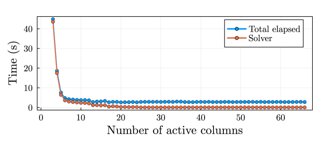
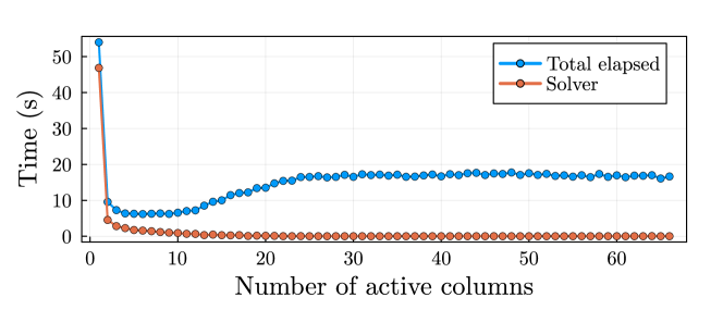
Figure 1: Average BCD iteration time for $n=127$, $m=66$ (top) and $n=257$, $m=130$ (bottom). In each case, the variable subset size $|S|=25$, and the number of indices in each active column is limited to $\lceil|S|/|C_{S}|\rceil$ (i.e., the indices were roughly evenly divided among the active columns). Each plotted point is the average of $30$ runs, where each run was computed using a random code family and random indices $S$. We show both the total time taken to form and solve the partial minimization problems, as well as the time taken by only the solver (Gurobi).

4.3 Comparison of BCD methods

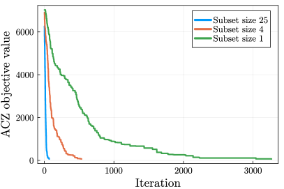
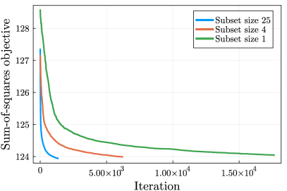
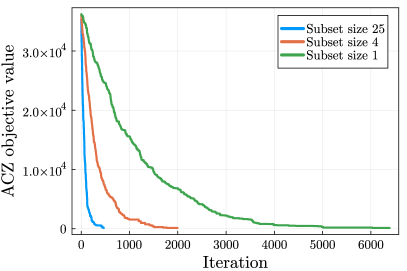
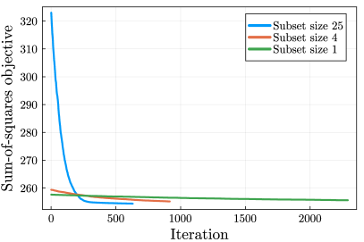
Figure 2: Top: objective value vs. iteration for stage-one (left) and stage-two (right) BCD, for problem setting $n=127$. Bottom: objective value vs. iteration for stage-one (left) and stage-two (right) BCD, for problem setting $n=257$. Stage-one BCD (left) is terminated when the ACZ property is satisfied. Objective values for stage-two BCD (right) are shown for the first hour of computation.

Next, we evaluate the performance of the two-stage BCD method with variable subset sizes $|S|=25$, $|S|=4$, and $|S|=1$.

Variable subset selection strategy.

We use the following selection scheme, which is based on the results in Subsection 4.2. In the $n=127$ case, the variable indices were selected by choosing a single variable index from $|S|$ different columns. In the $n=257$ case, the variable indices were selected by choosing the indices at random, with the constraint that the number of the number of active columns and the number of variable indices in each active column were limited to five each.

Results.

Figure 2 shows the objective value vs. iteration for the three subset sizes. The top left and bottom left plots show the ACZ objective value (8) vs. iteration for the first stage of BCD, for the $n=127$ and $n=257$ problem settings, respectively. The first stage is terminated when the ACZ constraint is satisfied. The top right and bottom right plots show the mean-of-squares metric (9) vs. iteration for the second stage of BCD, for the $n=127$ and the $n=257$ problem settings, respectively. The plots show the objective values for the first hour of computation.

In each case, it can be seen that increasing the subset size $|S|$ leads to a lower objective in fewer iterations, but also fewer total iterations, since the cost of each iteration is higher. Table 1 compares the mean-of-squares of the BCD-optimized codes with the Gold and Weil codes, where the BCD methods were run for $12$ hours. The BCD-optimized code with $|S|=25$ found a code with the lowest mean-of-squares in both problem settings. Table 2 shows the number of BCD iterations taken in the $12$ hour period, for each subset size $|S|$.

Autocorrelation visualization.

Finally, Figure 3 shows a superposition of the autocorrelations of the codes found using the BCD method with subset size $25$, compared with a superposition of the autocorrelations of the Gold and Weil codes. Both the BCD-optimized codes and the selected Gold codes satisfy the ACZ constraint, while it may be seen that the Weil codes do not. The BCD-optimized codes appear to strictly outperform the Weil codes. While the BCD-optimized codes appear to have autocorrelation closer to zero than the Gold codes on average, they have a larger peak autocorrelation magnitude than the Gold codes.

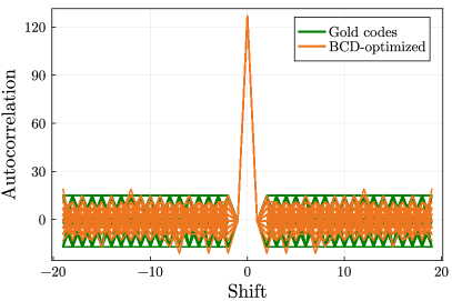
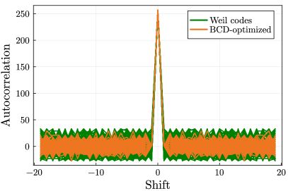
Figure 3: Autocorrelation of one of the 66 optimized binary sequence, compared with the autocorrelation of one of the Gold codes.

Table 1: Comparison of mean-of-squares of BCD optimized codes with Gold and Weil codes. In the $n=127$ case, BCD was used to optimize over $m=66$ codes, while there were only $m=65$ corresponding Gold codes. In the $n=257$ case, BCD was used to optimize over $m=130$ codes, whereas there were only $m=128$ Weil codes. The BCD-optimized and Gold codes satisfy the ACZ constraint, while the Weil codes do not.

	$n=127$	$n=257$
BCD ($|S|=25$)	123.741	253.707
BCD ($|S|=4$)	123.745	254.092
BCD ($|S|=1$)	123.762	254.234
Gold	125.95	-
Weil	-	255.99

Table 2: Number of BCD iterations taken in a 12-hour period, for different subset sizes $|S|$.

	$n=127$	$n=257$
$|S|=25$	15,756	8,680
$|S|=4$	70,966	10,278
$|S|=1$	209,966	26,671

5 Conclusions

In this work, we considered the problem of designing binary spreading codes with good auto- and cross-correlation properties, in particular for LEO applications, where the number of codes are large, relative to the code lengths. We proposed a two-stage BCD method for finding codes of arbitrary length and family size that both satisfy the ACZ property and have good correlation properties. We demonstrated that the method can find codes that outperform the Gold and Weil codes in terms of the mean of squared correlation values.

Finally, we discuss possible directions for future work. First, the BCD method proposed in this work may be extended to account for the effects of Doppler shift, which can be significant in LEO navigation settings [44]. For example, the BCD method may be used to optimize the average of the objective function (2a) over a range of Doppler shifts [45]. Second, this work did not consider the effects of any data or secondary codes, which are often superimposed on the primary spreading codes [12]. Those superimposed codes may adversely affect the correlation properties of the primary codes, and may be worth consideration in future work.

Declarations

Ethics approval and consent to participate

Not applicable.

Consent for publication

Not applicable.

Availability of data and materials

The datasets generated and/or analysed during the current study are available in the binary_seq_opt repository, https://github.com/Stanford-NavLab/binary_seq_opt

Competing interests

The authors declare that they have no competing interests.

Funding

This material is based upon work supported by the Air Force Research Lab (AFRL) under grant number FA9453-20-1-0002.

Authors’ contributions

AY formulated an extension of the MICP formulation from prior work, using the ASZ property, and implemented and ran the experiments. TM assisted in the experiment setup with the computing cluster, design of the experiments for the LEO navigation setting and code design objectives. GG assisted in ideation of the problem context for LEO navigation. All authors read and approved the final manuscript.

Acknowledgments

Not applicable.

References

- \bibcommenthead
- Reid et al. [2020] Reid, T.G., Walter, T., Enge, P.K., Lawrence, D., Cobb, H.S., Gutt, G., O’Connor, M., Whelan, D.: Navigation from low earth orbit: part 1: concept, current capability, and future promise. Position, Navigation, and Timing Technologies in the 21st Century: Integrated Satellite Navigation, Sensor Systems, and Civil Applications 2, 1359–1379 (2020)
- Maine et al. [1995] Maine, K., Devieux, C., Swan, P.: Overview of IRIDIUM satellite network. In: Proceedings of WESCON’95, p. 483 (1995). IEEE
- De Selding [2015] De Selding, P.B.: Virgin, Qualcomm invest in OneWeb satellite internet venture. Space News 15 (2015)
- Khan [2015] Khan, F.: Mobile internet from the heavens. arXiv preprint arXiv:1508.02383 (2015)
- De Selding [2015] De Selding, P.B.: SpaceX to build 4,000 broadband satellites in seattle. Space news 19 (2015)
- Septentrio [2023] Septentrio: Septentrio collaborates with Xona on PULSAR GNSS receiver. Accessed: 19 June 2023 (2023). https://www.septentrio.com/en/company/news/septentrio-collaborates-xona-pulsar-gnss-receiver
- Reid et al. [2016] Reid, T.G., Neish, A.M., Walter, T.F., Enge, P.K.: Leveraging commercial broadband LEO constellations for navigating. In: Proceedings of the 29th International Technical Meeting of the Satellite Division of the Institute of Navigation (Ion Gnss+ 2016). 29th International Technical Meeting of the Satellite Division of the Institute of Navigation (Ion Gnss+ 2016), Portland, Oregon, vol. 12, pp. 2016–16 (2016)
- Dennehy [2023] Dennehy, K.: Is LEO PNT the next big thing?, vol. 33 (2023). https://www.ion.org/publications/upload/ION-Winter2023.pdf
- Prol et al. [2022] Prol, F.S., Ferre, R.M., Saleem, Z., Välisuo, P., Pinell, C., Lohan, E.-S., Elsanhoury, M., Elmusrati, M., Islam, S., Çelikbilek, K., et al.: Position, navigation, and timing (PNT) through low earth orbit (LEO) satellites: A survey on current status, challenges, and opportunities. IEEE Access (2022)
- Misra and Enge [2012] Misra, P., Enge, P.: Global positioning system: Signals, measurements & performance. Ganga-Jamuna Press (2012)
- Bekhit et al. [2011] Bekhit, H.B., El Diwany, E., El Ramly, S.H.: Design of ranging codes for low-earth orbit satellites. In: Proceedings of 5th International Conference on Recent Advances in Space Technologies (RAST), pp. 324–329 (2011). IEEE
- Wallner et al. [2007] Wallner, S., Avila-Rodriguez, J.-A., Hein, G.W., Rushanan, J.J.: Galileo E1 OS and GPS L1C pseudo random noise codes-requirements, generation, optimization and comparison. In: Proceedings of the 20th International Technical Meeting of the Satellite Division of The Institute of Navigation (ION GNSS 2007), pp. 1549–1563 (2007)
- Winkel [2011] Winkel, J.O.: Spreading codes for a satellite navigation system. United States Patent. Patent No.: US 8,035,555 B2 (2011)
- Conforti et al. [2014] Conforti, M., Cornuéjols, G., Zambelli, G.: Integer programming. vol. 271. Springer (2014)
- Yang et al. [2023a] Yang, A., Mina, T., Gao, G.: Binary sequence set optimization for CDMA applications via mixed-integer quadratic programming. In: IEEE International Conference on Acoustics, Speech, & Signal Processing (2023)
- Yang et al. [2023b] Yang, A., Mina, T., Gao, G.: Spreading code sequence design via mixed-integer convex optimization. In: Proceedings of the 36th International Technical Meeting of the Satellite Division of The Institute of Navigation (ION GNSS+ 2023), pp. 1341–1351 (2023)
- Gurobi Optimization [2022] Gurobi Optimization, L.: Gurobi Optimizer Reference Manual (2022). https://www.gurobi.com
- Gold [1967] Gold, R.: Optimal binary sequences for spread spectrum multiplexing. IEEE Transactions on information theory 13(4), 619–621 (1967)
- Rushanan [2007] Rushanan, J.J.: The spreading and overlay codes for the L1C signal. Navigation 54(1), 43–51 (2007)
- Legendre [1808] Legendre, A.-M.: Essai sur la théorie des nombres. Chez Courcier (1808)
- Mina and Gao [2019] Mina, T.Y., Gao, G.X.: Devising high-performing random spreading code sequences using a multi-objective genetic algorithm. In: Proceedings of the 32nd International Technical Meeting of the Satellite Division of The Institute of Navigation (ION GNSS+ 2019), pp. 1076–1089 (2019)
- Liu et al. [2022] Liu, T., Sun, J., Wang, G., Lu, Y.: A multi-objective quantum genetic algorithm for MIMO radar waveform design. Remote Sensing 14(10), 2387 (2022)
- Mina and Gao [2022] Mina, T.Y., Gao, G.X.: Designing low-correlation GPS spreading codes with a natural evolution strategy machine-learning algorithm. NAVIGATION, Journal of the Institute of Navigation 69(1) (2022)
- Mina et al. [2023] Mina, T., Yang, A., Gao, G.: Designing long gps memory codes using the cross entropy method. In: Proceedings of the 36th International Technical Meeting of the Satellite Division of The Institute of Navigation (ION GNSS+ 2023), pp. 1328–1340 (2023)
- Wallner et al. [2008] Wallner, S., Avila-Rodriguez, J.-A., Won, J.-H., Hein, G., Issler, J.-L.: Revised PRN code structures for galileo E1 OS. In: Proceedings of the 21st International Technical Meeting of the Satellite Division of The Institute of Navigation (ION GNSS 2008), pp. 887–899 (2008)
- Alaee-Kerahroodi et al. [2019] Alaee-Kerahroodi, M., Modarres-Hashemi, M., Naghsh, M.M.: Designing sets of binary sequences for MIMO radar systems. IEEE Transactions on Signal Processing 67(13), 3347–3360 (2019)
- Cui et al. [2017] Cui, G., Yu, X., Foglia, G., Huang, Y., Li, J.: Quadratic optimization with similarity constraint for unimodular sequence synthesis. IEEE Transactions on Signal Processing 65(18), 4756–4769 (2017)
- Lin and Li [2020] Lin, R., Li, J.: On binary sequence set design with applications to automotive radar. In: ICASSP 2020-2020 IEEE International Conference on Acoustics, Speech and Signal Processing (ICASSP), pp. 8639–8643 (2020). IEEE
- Huang and Lin [2020] Huang, W., Lin, R.: Efficient design of Doppler sensitive long discrete-phase periodic sequence sets for automotive radars. In: 2020 IEEE 11th Sensor Array and Multichannel Signal Processing Workshop (SAM), pp. 1–5 (2020). IEEE
- Yuan et al. [2017] Yuan, G., Shen, L., Zheng, W.-S.: A hybrid method of combinatorial search and coordinate descent for discrete optimization. arXiv preprint arXiv:1706.06493 (2017)
- Yu et al. [2020] Yu, X., Cui, G., Yang, J., Li, J., Kong, L.: Quadratic optimization for unimodular sequence design via an ADPM framework. IEEE Transactions on Signal Processing 68, 3619–3634 (2020)
- De Maio et al. [2008] De Maio, A., De Nicola, S., Huang, Y., Zhang, S., Farina, A.: Code design to optimize radar detection performance under accuracy and similarity constraints. IEEE Transactions on Signal Processing 56(11), 5618–5629 (2008)
- Bose and Soltanalian [2018] Bose, A., Soltanalian, M.: Constructing binary sequences with good correlation properties: An efficient analytical-computational interplay. IEEE Transactions on Signal Processing 66(11), 2998–3007 (2018)
- Boukerma et al. [2021] Boukerma, S., Rouabah, K., Mezaache, S., Atia, S.: Efficient method for constructing optimized long binary spreading sequences. International Journal of Communication Systems 34(4), 4719 (2021)
- Medina et al. [2020] Medina, D., Ortega, L., Vilà-Valls, J., Closas, P., Vincent, F., Chaumette, E.: Compact CRB for delay, Doppler, and phase estimation–application to GNSS SPP and RTK performance characterisation. IET Radar, Sonar & Navigation 14(10), 1537–1549 (2020)
- Ortega et al. [2020] Ortega, L., Vilà-Valls, J., Chaumette, E., Vincent, F.: On the time-delay estimation performance limit of new GNSS acquisition codes. In: 2020 International Conference on Localization and GNSS (ICL-GNSS), pp. 1–6 (2020). IEEE
- He et al. [2012] He, H., Li, J., Stoica, P.: Waveform design for active sensing systems: a computational approach. Cambridge University Press (2012)
- Glover and Woolsey [1974] Glover, F., Woolsey, E.: Converting the 0-1 polynomial programming problem to a 0-1 linear program. Operations Research 22(1), 180–182 (1974)
- Bestuzheva et al. [2021] Bestuzheva, K., Besançon, M., Chen, W.-K., Chmiela, A., Donkiewicz, T., Doornmalen, J., Eifler, L., Gaul, O., Gamrath, G., Gleixner, A., et al.: The SCIP optimization suite 8.0. arXiv preprint arXiv:2112.08872 (2021)
- Lawler and Wood [1966] Lawler, E.L., Wood, D.E.: Branch-and-bound methods: A survey. Operations research 14(4), 699–719 (1966)
- Brucker et al. [1994] Brucker, P., Jurisch, B., Sievers, B.: A branch and bound algorithm for the job-shop scheduling problem. In: Discrete Applied Math, vol. 49, pp. 107–127 (1994)
- Padberg and Rinaldi [1991] Padberg, M., Rinaldi, G.: A branch-and-cut algorithm for the resolution of large-scale symmetric traveling salesman problems. SIAM Rev. (33), 60–100 (1991)
- Stubbs and Mehrotra [1999] Stubbs, R., Mehrotra, S.: A branch-and-cut method for 0-1 mixed convex programming. Math. Program. (86), 515–532 (1999)
- Soualle et al. [2005] Soualle, F., Soellner, M., Wallner, S., Avila-Rodriguez, J.-A., Hein, G.W., Barnes, B., Pratt, T., Ries, L., Winkel, J., Lemenager, C., et al.: Spreading code selection criteria for the future GNSS Galileo. In: Proceedings of the European Navigation Conference GNSS, pp. 19–22 (2005)
- Yang et al. [2024] Yang, A., Mina, T.Y., Gao, G.X.: Fast spreading code optimization under doppler effects. In: Proceedings of the 2024 International Technical Meeting of The Institute of Navigation (ION ITM 2024) (2024)