[2404.12379] “Dynamic Gaussians Mesh: Consistent Mesh Reconstruction from Monocular Videos” Supplementary Material

Appendix 0.A Overview

In this supplementary material, we first introduce more implementation details in Appendix 0.B, including the network architecture, the detailed description of our Gaussian-Mesh Anchoring algorithm, and the training details. In Appendix 0.C, we introduce more information on our rendered dataset. In Appendix 0.D, we show more mesh construction results of our method compared with other baselines on the D-NeRF dataset as well as the DG-Mesh dataset.

Appendix 0.B Implementation Details

0.B.1 Network Architecture and Training Details

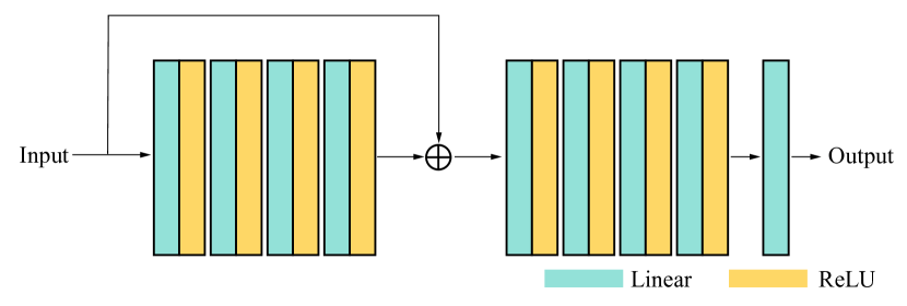
For the forward and backward deformation networks, we use an MLP the depth $D=8$ and the dimension of the hidden layer $W=256$ . An illustration of the network architecture is shown in Fig. 1. We apply positional encoding $\gamma^{k}(p)$ to map position $x$ and time label $t$ to higher dimensional feature space, and we set $k=10$ for 3D Gaussian’s positions $x$ and $k=6$ for time label $t$ . After the last layer, we use a single Linear layer without activation to obtain the predicted Gaussian position offset $\delta x$ , scaling offset $\delta s$ , rotation offset $\delta r$ and the opacity offset $\delta\alpha$ . The appearance network uses the similar architecture as the deformation network, while the last layer outputs the RGB color of the input vertex.

Refer to caption — Figure 1: Illustration of the network architecture

During training, we train the first $3k$ iterations without optimizing the parameters in the deformation network, this helps to retain relatively stable positions and shapes of 3D Gaussians under the canonical space. From iteration $8k$ , we start to optimize the mesh and its appearance using Differentiable Poisson Solver (DPSR) and Differentiable Marching Cubes (Diff. MC). Starts from iteration $15k$ , we perform the Gaussian-Mesh Anchoring every $100$ iterations guide the Gaussian points more uniformly distribute on the surface. We train the network for $50k$ iterations in total.

0.B.2 Gaussian-Mesh Anchoring Algorithm

We use the Gaussian-Mesh Anchoring procedure to guide the Gaussian to be more uniformly distributed on the object’s surface, which results in a smoother mesh reconstruction from DPSR and DiffMC. In Algorithm 1 is a more detailed description of our algorithm. The algorithm first find the nearest mesh face for each Gaussian point. For each mesh face, if it is linked to multiple Gaussian points, merge these Gaussians and creat a new one. If a mesh face is only linked to one specific Gaussian, we move this Gaussian towards the face centroid. If a mesh face is not linked to any Gaussian point, we create a new Gaussian using the face centroid.

Data: gaussians, time, verts, faces, deform, deform_back, search_radius=0.005

Result: anchor_loss

deformed_gaussian = deform(gaussians, time);

anchor_loss = 0;

for face in faces do

gs_to_mesh_idx = knn(deformed_gaussian, face.centroid, k=1, radius=search_radius);

selected_gaussians = gaussians[gs_to_mesh_idx == face];

if count(selected_gaussians) > 1 then

new_gaussian = merge_gaussians(selected_gaussians);

canonical_new_gaussian = deform_back(new_gaussian, time);

gaussians.delete(selected_gaussians);

gaussians.append(canonical_new_gaussian);

anchor_loss += distance(canonical_new_gaussian, face);

end if

else if count(gs_to_mesh_idx == face) == 1 then

anchor_loss += distance(selected_gaussians, face);

end if

else

new_gaussian = face.centroid;

canonical_new_gaussian = deform_back(new_gaussian, time);

gaussians.append(canonical_new_gaussian);

end if

end for

Algorithm 1 Gaussian-Mesh Anchoring

Appendix 0.C Dataset Details

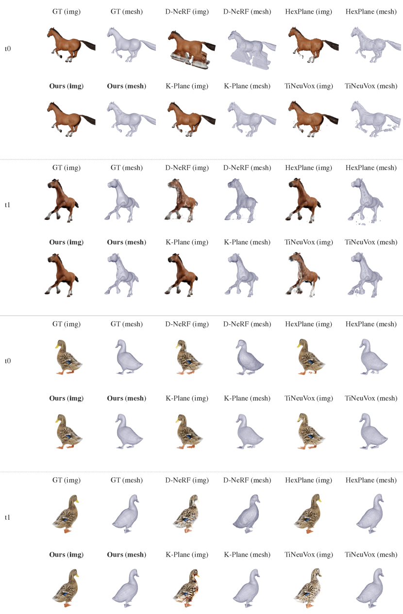
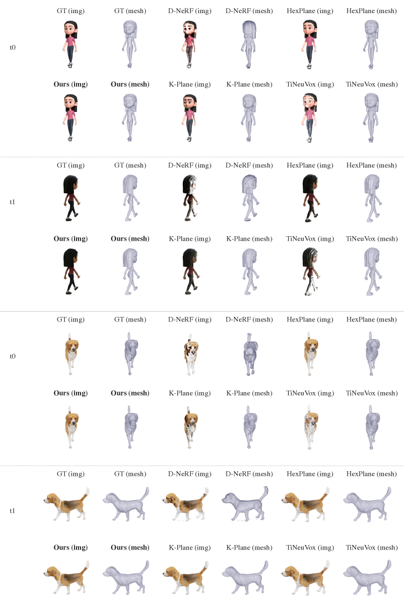
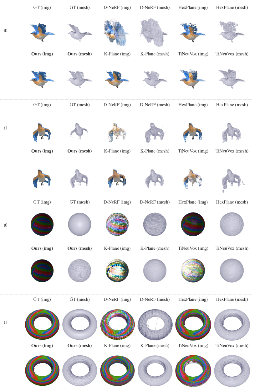
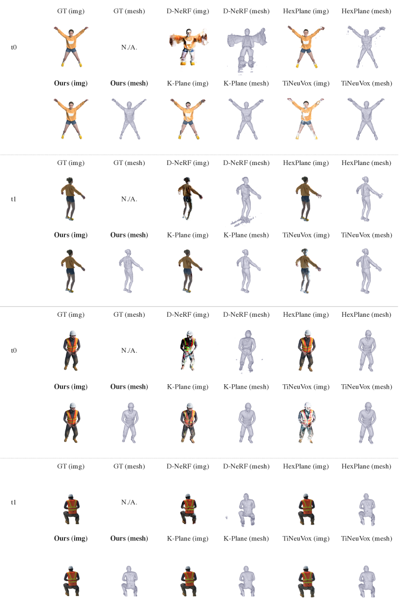
To quantitatively evaluate the mesh reconstruction quality of our method, ground truth mesh is needed. Since the existing dataset (e.g. the D-NeRF dataset) does not provide mesh ground truth information, we use Blender to render our own dataset. Specifically, we render 6 dynamic scenes including a running horse, a flying bird, a walking beagle, a walking duck, a walking cartoon girl, and a deforming sphere. The deforming sphere example is designed to test the method’s ability to handle topology change during deformation (the sphere is gradually deformed into a torus). Our dataset follows the data format from the D-NeRF dataset, which provides camera parameters, RGB images, as well as the ground truth mesh stored in OBJ format.

For rendering specification, we use the Eevee render engine for the running horse scene and the Cycles render engine for the other five scenes. The sampling number is set to 128. The video length for each scene is 200 frames. For both training and testing sets, each frame is only visible under one camera view. The rendered image resolution is $800\times 800$ in s-RGB color space.

Appendix 0.D Results on the D-NeRF and DG-Mesh Dataset

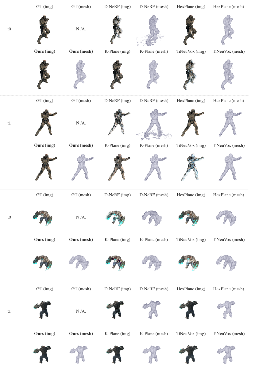
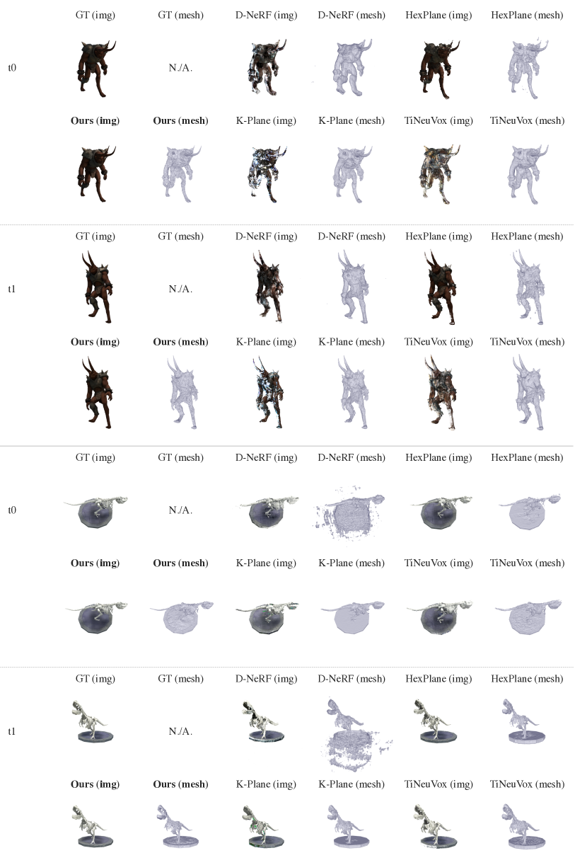
We provide more results visualization of our method as well as the other baselines on the D-NeRF dataset and the DG-Mesh dataset. From Fig. 2 - Fig. 4 are the results on the DG-Mesh dataset. For each data sample, We show the reconstructed mesh and mesh rendering image under two different time frame and camera view. The results shows our method achieves best mesh reconstruction as well as rendering quality. From Fig. 5 - Fig. 8 are the results on the D-NeRF dataset, our method also gives both mesh reconstruction and rendering quality in general.