6Img-to-3D: Few-Image Large-Scale Outdoor Driving Scene Reconstruction

Abstract

Current 3D reconstruction techniques struggle to infer unbounded scenes from a few images faithfully. Specifically, existing methods have high computational demands, require detailed pose information, and cannot reconstruct occluded regions reliably. We introduce 6Img-to-3D, an efficient, scalable transformer-based encoder-renderer method for single-shot image to 3D reconstruction. Our method outputs a 3D-consistent parameterized triplane from only six outward-facing input images for large-scale, unbounded outdoor driving scenarios. We take a step towards resolving existing shortcomings by combining contracted custom cross- and self-attention mechanisms for triplane parameterization, differentiable volume rendering, scene contraction, and image feature projection. We showcase that six surround-view vehicle images from a single timestamp without global pose information are enough to reconstruct 360^∘ scenes during inference time, taking 395 ms. Our method allows, for example, rendering third-person images and birds-eye views. Our code is available here, and more examples can be found at our website https://6Img-to-3D.GitHub.io/.

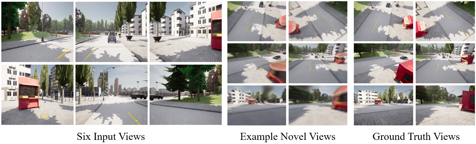
Figure 1: Qualitative results of 6Img-to-3D. During inference time, 6Img-to-3D takes six surround vehicle RGB images as input and returns a parameterized triplane from which arbitrary views can be rendered.

1 Introduction

Inferring the appearance and geometry of large-scale outdoor scenes from a few camera inputs is a challenging, unsolved problem. The problem is characterized by the complexity inherent in outdoor scenes, namely a vast spatial extent, diverse object textures, and ambiguity of the 3D geometry when resolving occlusions. Robotics and autonomous driving systems both require methods that process vision-centric first-person views from a fixed set of cameras as input and derive suitable control commands from these [80]. The ability to instantaneously perform 2D-to-3D scene reconstructions would be useful within such methods and thus have a broad applicability within the robotics [2, 51, 60, 89] and autonomous driving [61, 15, 111, 8] domains. Instantaneously generating unoccluded bird’s-eye views in difficult parking or slow driving scenarios would, for example, greatly assist human drivers. For applying one-shot images to high-fidelity 3D techniques in vehicles or robots, additional factors, such as the inference speed, the quality of the inferred representation, the scalability of the approach, and the number of camera parameters required for the technique to work, are equally important. For those safety-critical domains, avoiding overly compressing the 3D scene or altering scene details by adding or omitting road obstacles is crucial. For those safety-critical domains, avoiding overly compressing the 3D scene or altering scene details by adding or omitting road obstacles is crucial.

Despite recent progress in 3D reconstruction from a few or single 2D images, many methods are either limited to single objects [27, 76, 46, 45, 96] or to generative indoor view synthesis [12]. Existing few-shot methods developed for single objects are often not easily transferable to large-scale or unbounded outdoor settings. This is because outdoor settings are more diverse due to their varying structural composition, occlusions, and vast extent. Another limitation is that many methods require a high degree of overlap between the input images, such as found in spherically arranged and inward-facing camera setups focused on a single object in the center [55, 103]. This is opposed to the outward-facing camera setup essential for autonomous driving where the camera overlap is minimal [6, 9, 74]. The camera setups are contrasted in Fig. 2. Traditional methods in autonomous driving have shown promising results with such camera setups but lack visual fidelity since they only predict semantic occupancy [28, 81, 72, 87] and commonly rely on additional sensors such as LiDAR.

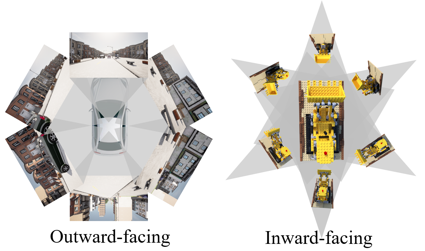
Figure 2: View Overlap. Inward and outward-facing camera setups differ significantly in their view overlap. Ourward-facing (inside-out) camera setups overlap minimally, whereas inward-facing (outside-in) setups can overlap across multiple cameras. The source of the excavator images is [54, 55].

Given the above limitations, we present 6Img-to-3D, a novel transformer-based decoder-renderer method for single-shot image to 3D reconstruction. 6Img-to-3D is fully differentiable and end-to-end trained on a single GPU. It simultaneously takes six outward-facing images (6 Img) as inputs and generates a parameterized triplane (to 3D) from which novel scene views can be rendered. Unlike previous methods, we do not focus on single objects but instead on complex driving scenarios characterized by a high-depth complexity recorded only by sparse multi-view outward-facing RGB cameras. Furthermore, unlike other methods, we do not use a multi- or few-shot scheme where an initial reconstruction is tested and improved iteratively. Instead, we provide the 3D reconstruction in a single shot without iterative model refinement. To this end, we utilize pre-trained ResNet features, cross- and self-attention mechanisms for parameterizing the triplane, and image feature projection to condition the renderer. Our method has 61M parameters and is trained using roughly 11.4K input and 190K supervising images from 1900 scenes. We do not require depth or LiDAR information. Due to the absence of suitable datasets, including a large number of non-ego vehicle views needed during training, we rely on synthetic data from Carla [19].

The contributions of this paper can be summarized as follows:

1. Visual Fidelity and Unboundedness. We present 6Img-to-3D, an efficient, single-shot, few-image reconstruction pipeline for large-scale outdoor environments. Our method outputs a parameterized triplane of the 3D scene from which arbitrary viewpoints can be rendered. We combine triplane-based differentiable volume rendering, renderer conditioning on projected image features, self- and custom cross-attention mechanisms, and an LPIPS loss.

2. Scaling and Hardware Efficiency. We demonstrate the favorable scaling properties of our architecture regarding the amount of training data. Unlike other large-scale 2D-to-3D methods, 6Img-to-3D trains and runs on a single 42GB GPU, allowing easier transfer of the method to embedded systems.

3. Testing and Abblations. We perform extensive additional tests and ablation studies to confirm the effect of individual model components such as the LPIPS loss, projected image features conditioning, and scene contraction.

4. Self-Supervised and Runtime. We establish that our method trained by using self-supervised learning generalizes well to novel scenes without inputting additional camera poses other than those required to define the novel views. Since our method only requires a single-forward pass during inference, obtaining a parameterized triplane is fast and only takes 395ms.

Our code is available here.

2 Related Work

3D Representations. Traditional methods for representing 3D scenes include voxels [68, 24, 91, 97, 88, 75], point clouds [20, 105, 100, 1, 106, 75], signed distance field (SDF) [84, 38] and polygon meshes [75, 32, 83, 57, 94, 48]. Recently, numerous new implicit and explicit representations have emerged for learning 3D scenes [79, 92, 23]. Implicit neural fields such as Neural Radiance Fields (NeRFs) model the surrounding appearance and geometry using a continuously queriable function. They can be updated through differentiable volumetric rendering [59, 55, 49, 77, 23] and either utilize a single [17, 55, 108] or multiple [66, 64] multilayer perceptrons (MLPs). However, these models are slow to train, data-intensive, and expensive to render since querying the implicit neural field is computationally demanding. Explicit approaches such as Plenoctrees [102], Plenoxels [101], and NSVF [44] employ trilinear interpolation within a 3D grid to represent the scene. This significantly improves rendering and optimization time but comes at the expense of limited scalability due to the curse of dimensionality when increasing the resolution or scene size. Hybrid models [73, 56] adopt an intermediary representation, storing values in a voxel-like grid. These values are then decoded using viewing direction through a shallow MLP to infer color and density. Some models further refine this process by decomposing the voxel grid into vector-matrix, using the CANDECOMP/PARAFAC (CP) decompositions [13] or into three or more orthogonal planes called triplanes or K-Planes [11, 5, 21]. This enables the computation of features for each point in space by aggregating the feature values of projected 3D points onto each plane, transitioning from an N-cube voxel grid to a 3 $\times$ N-squared plane representation.

Few-Image to 3D Representation. Single-scene 3D reconstruction methods require many images to generalize towards novel views since the reconstruction problem would be underconstrained otherwise [55]. Hence, few-image to 3D representation methods incorporate additional global or local information to further regularize and constrain the problem. Global regularization methods rely on additional model priors, either via applying further model regularization [98, 58] or by utilizing pre-trained image models to provide an extra guidance signal to inform the optimization of the single-scene [18, 63, 45, 53, 69, 93, 96, 42, 62]. Local regularization methods train a cross-scene multi-perspective aggregator. Such models include PixelNeRF [103], IBRNet [85], MVSNeRF [14], VolRecon [67] and others [82, 47, 31, 40]. They retrieve image features via view projection and aggregate resulting features using MLPs or transformers to obtain novel views. We also rely on pixel feature conditioning, but unlike our method, many of the mentioned local regularization methods rely on a large overlap between input images ensured by using spherical inward-facing cameras. Another category of methods does not train the representation on a per-scene basis but instead trains a meta-network that outputs the discrete parameterized scene representation. Models such as [71, 22, 25, 3, 86] use diffusion to generate 3D representations of scenes. Many of those models use the triplane representation [71, 22, 25, 3], whereas some directly generate in the image-space [86] or can be conditioned on input images [25, 86, 3]. Other methods [11, 7] use GANs to generate 3D representations. The method that most closely resembles our work is LRM [27], which utilizes cross- and self-attention to parameterize a triplane using a few object images. LRM focuses on single objects and does not handle unbound scenes. In addition, we train on a single A40 GPU, whereas LRM is trained on 128 NVIDIA A100 GPUs and has seven times more parameters.

Large-Scale 3D Scene Representations. Extending NeRFs to unbounded scenes requires spatially contracting the scene is usually done proportionally to disparity as introduced in MipNeRF-360 [4] or using an inverted sphere parametrization as in NeRF++ [109]. Architectures modeling outdoor driving scenes are BlockNeRF [78], Neural Scene Graphs [61], DisCoScene [95], NeuralField-LDM [33] and Neural ground planes [70]. Those are, however, not dealing with sparse input views. Neo360 [30] utilizes local image features to infer an image-conditional triplanar representation, whereby the model dissociates foreground from background scene parts. Unlike our method, Neo360 is trained on 8 A100 GPUs and focuses on inward-facing camera perspectives as input to the model. Due to the larger view overlap, Neo360 thus solves an easier 2D-to-3D lifting task. Large-scale scene generation methods such as Infinite Nature [43], InfiniteNature-Zero [36], PathDreamer [35], CityDreamer [90], Infinicity [39], SceneDreamer [16] and PersistentNature [10] often produce additional images in an autoregressive fashion without the ability to input camera coordinates for novel view synthesis control. In autonomous driving, 3D visual perception tasks include 3D detection and map segmentation based on multi-camera images. Established methods create a bird’s-eye-view (BEV) semantic representation of a scene using either Inverse Perspective Mapping (IPM) [65] or attention mechanisms [99, 37]. TPVFormer [29], a work that our architecture is partially based on, maps six outward-facing vehicle 2D images onto three orthogonal planes using self- and cross-deformable attention mechanisms to obtain semantic occupancy predictions. The method is, however, supervised with depth information from a LiDAR sensor and, unlike our method, only predicts semantic occupancy.

3 6Img-to-3D

Given six outward-facing images $\bm{I}_{ego}$, their camera extrinsic (relative pose) matrices $\bm{M}$ and associated camera intrinsic matrices $\bm{K}$ with appropriate dimensions, the goal is to reconstruct the surrounding 3D occupancy and appearance, that is the scene $\bm{S}$. Since the values of the scene $\bm{S}$ are not known, we use ${N}$ spherical multi-view images $\bm{I}_{sphere}$ with their associated extrinsic and extrinsic matrices during training as a supervision signal to estimate the scene $\bm{\hat{S}}$. The proposed architecture for lifting $\bm{I}_{ego}$ consists of an image-to-triplane encoder. After a forward pass through this architecture, the discrete triplane contains the approximation of the scene $\bm{\hat{S}}$. The following sections describe the different parts of the pipeline visualized in Fig. 3 and the training objectives.

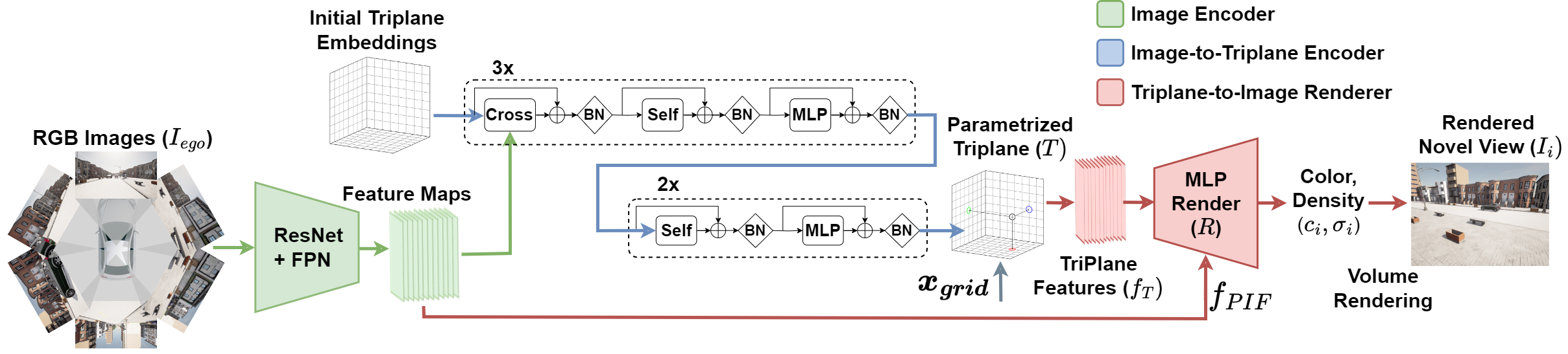
Figure 3: The overview of 6Img-to-3D. Given six input images, we first encode them into feature maps using a pre-trained ResNet and an FPN (Sec. 3.1). The scene coordinates are contracted to fit the unbounded scenes (Sec. 3.2). MLPs, cross-and self-attention layers form the Image-to-Triplane Encoder of our framework (Sec. 3.3). Images can be rendered from the resulting triplane using our renderer (Sec. 3.4). We additionally condition the rendering process on projected image features.

3.1 Image Encoder

Six RGB input images $\bm{I}_{ego}\in\mathbb{R}^{6\times 3\times H\times W}$ are processed via a pre-trained ResNet [26] followed by a Feature Pyramid Network (FPN) [41], resulting in multi-scale pixel-aligned image features $\bm{F}_{I}\in\mathbb{R}^{6\times 3\times H/i\times W/i},$ with $i=\{8,16,32,64\}$.

3.2 Triplane Representation

The triplane consists of three pairwise orthogonal feature grids ${\bm{T}_{HW}}$, ${\bm{T}_{HZ}}$ and ${\bm{T}_{WZ}}$, each representing parts of the decomposed 3D space, a setup similar to EG3D [11]. We choose triplanes because they allow gradient-based optimization, are explicit representations and their parameterization is thus straightforward. Additionally, they are lightweight and provide an easily queriable information encoding [11, 21]. The triplane ${\bm{T}}$ is composed of the three coordinate-centered and axis-aligned planes ${\bm{T}_{HW}}$, ${\bm{T}_{HZ}}$ and ${\bm{T}_{WZ}}$, respectively of size $200\times 200\times F_{T}$, $200\times 16\times F_{T}$ and $200\times 16\times F_{T}$, where $F_{T}$ is the number of feature channels of the triplane. Due to the concentration of relevant information near the ground plane in 3D outdoor driving scenes, we decide to allocate more space to the horizontal dimensions ($HW$) than to the vertical dimension ($Z$). The grid coordinates $\bm{x_{grid}}$ for each plane are normalized between -1 and 1. The contraction equation from world coordinates $\bm{x_{w}}$ to grid coordinates $\bm{x_{grid}}$ is given as element-wise operations by

$$\begin{split}\bm{x_{Ws}}&=\bm{x_{W}}\cdot\bm{s}\\ \bm{x_{grid}}&=\begin{cases}\text{${\frac{\bm{x_{Ws}}}{2}}$}&\text{$\|\bm{x_{Ws}}\|\leq 1$}\\ \text{$(2-\frac{1}{\|\bm{x_{Ws}}\|})\frac{\bm{x_{Ws}}}{2\|\bm{x_{Ws}}\|}$}&\text{$\|\bm{x_{Ws}}\|>1$}\end{cases}\end{split}$$ (1)

In short, a scaling parameter $\bm{s}=[s_{h},s_{w},s_{z}]$ is applied before contraction to adapt to the nature of our scenes, and the scaled world coordinates $\bm{x_{Ws}}$ are contracted using the spatial distortion introduced in Mip-NeRF 360 [4] to obtain $\bm{x_{grid}}$, with $||\cdot||$ denoting the L2 norm.

3.3 Image-to-Triplane Encoder

The Image-to-Triplane Encoder, adopted from TPVFormer [28], comprises deformable custom cross- and self-attention layers, both using residual connections. The first half of the encoder consists of three consecutive blocks of cross-attention, self-attention, and MLPs, and the second half consists of two blocks that only have self-attention layers and MLPs. The next sections will introduce each component in more detail. Intermediate batch normalization (BN) layers are applied within both blocks. The number of blocks is empirically motivated. We hypothesize that increasing the number of blocks could further improve performance; the current design reflects a balance chosen considering our computing constraints. LRM [27], for example, uses 16 blocks in total.

Cross-Attention (Image-Triplane) We use cross-attention to incorporate as much information as possible from input image features into the triplane grids. This is facilitated by deformable attention mechanisms (DeformAttn) [112]. Unlike traditional attention mechanisms, this layer is designed to handle the high dimensionality of both the image features and the triplanar grids by restricting the attention of each query to a small set of keys, rather than to all available keys as in traditional attention. This layer is applied to each plane separately. Establishing the link between each query (triplane feature) and its keys (image features) is non-trivial. We compute the deformable attention the following way:

$$\textbf{CrossAttn}(\bm{T_{k}})=\text{DeformAttn}(\bm{T_{k}},\bm{p^{F}_{k}},\bm{F_{I}}),k\in\{HW,HZ,WZ\}\$$

whereby the grid features $\bm{T_{k}}$ are used as queries, the image features $\bm{F_{I}}$ as keys and the reference points $\bm{p^{F}_{k}}$ links a selected number of keys to each query.

We establish the correspondence via reference points $\bm{p^{F}_{k}}$, computed as follows: we first establish a correspondence from camera indices $(u,v)_{cam_{i}}$ to world coordinates $\bm{x}_{\text{W}}$ by sampling points along each input camera ${cam_{i}}$ ray, as illustrated in Fig. 4a. The world coordinates $\bm{x}_{\text{W}}$ are then transformed into grid coordinates $\bm{x}_{\text{grid}}$, employing Eq. 1, as shown in Fig. 4b. Given the obtained correspondences between camera indices $(u,v)_{cam_{i}}$ and 3D grid coordinates, for each plane $\bm{T_{k}}$ we consider only a subset of $n_{k}$ fixed slices of the correspondences to obtain the reference points $p_{F}^{k}$, illustrated in Fig. 4c. For any $(i,j)$ index in the plane $\bm{T_{k}}$, we now have a correspondence to $n_{k}$ image feature indexes via the reference points $\bm{p^{F}_{k}}$. $n_{k}$ is proportional to the dimension perpendicular to the plane $\bm{T_{k}}$ ($4$ for ${\bm{T}_{HW}}$, $32$ for ${\bm{T}_{HZ}}$ and ${\bm{T}_{WZ}}$).

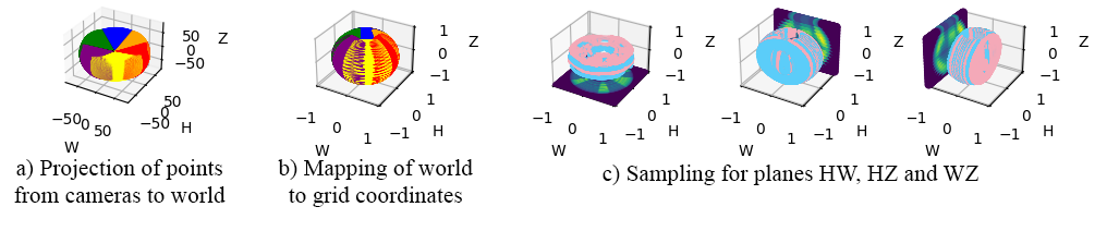
Figure 4: Establishing Reference Points. a) Points are projected into the world space from the cameras. b) Those points are mapped into the grid space. c) For each plane element, $n$ points are selected to be used as reference points between the grid index and image feature.

Self-Attention (Triplane) This layer is the same as the one within TPVFormer. It allows the three planes to exchange information between and within themselves. The self-attention layer also makes use of the deformable attention described above:

$$\textbf{SelfAttn}(\bm{T_{k}})=\text{DeformAttn}(\bm{T_{k}},\bm{p^{T}_{k}},\mathbf{T}),k\in\{HW,HZ,WZ\}\;.$$

whereby $\bm{T_{k}}$ is the plane used as query, the triplane $\mathbf{T}$ is used as keys and the query to keys correspondence is defined by the reference points $\bm{p^{T}_{k}}$. For any element in a plane, reference points are obtained by randomly sampling in their neighborhood and in their perpendicular direction.

3.4 Triplane-to-Image Renderer

The renderer $\bm{R}$, consisting of a shallow MLP, predicts the color $\bm{c}$ and density $\sigma\in[0,1]$ for a sampled 3D point $\bm{x_{W}}\in\mathbb{R}^{3}$. As we are dealing with Lambertian scenes, the view directions are discarded. The sampling point $\bm{x_{W}}$ is first converted into grid coordinates $\bm{x_{grid}}$ using Eq. 1. The triplane features $\bm{f_{T}}$ are then obtained by projecting this point via bilinear sampling onto each plane and applying the Hadamard product (elementwise multiplication) on those plane features: $\bm{f_{T}}^{ijk}=\bm{T}_{HW}(\bm{x_{grid}}^{ij})\cdot\bm{T}_{HZ}(\bm{x_{grid}}^{ik})\cdot\bm{T}_{WZ}(\bm{x_{grid}}^{jk})$.

Inspired by PixelNeRF [104], we extract the Projected Image Features $\bm{f_{PIF}}$ from the pixel-aligned input image features $\bm{F_{I}}$ by projecting $\bm{x_{W}}$ back into the image space of the input cameras: ${(u,v)}_{cam_{i}}=\bm{K}_{i}~{}\bm{M}_{i}^{-1}~{}{\bm{x_{W}}},i\in\{1,...,6\}$. Since each point in space can be seen by a maximum of two cameras, the aggregation function concatenates the valid features, with zero-padding when one or no camera sees the point: $\bm{f_{PIF}}=\text{aggregation}(F_{Ii}\text{(u,v)}_{cam_{i}}\text{ for }i\in\{1,...,6\})$.

As the triplane features $\bm{f_{T}}$ and the projected image features $\bm{f_{PIF}}$ come from two different distributions, we first process $\bm{f_{PIF}}$ through batch normalization before going through the renderer: $\bm{c},\sigma=\bm{R}(\bm{f_{T}},\textrm{BatchNorm}(\bm{f_{PIF}}))$. Given the volume density $\sigma_{i}$ and the color $\bm{c_{i}}$, we follow the same volume rendering equations as NeRF [55], originating from [52]. Initially, multiple coarse points are sampled uniformly along each ray $\bm{r}$. Those coarse points are then fed into the renderer to obtain densities, which are used for finer proportional sampling. The renderer then accumulates contributions from these points along the ray, which can be expressed as

$$\hat{C}(\bm{r})=\sum_{i=1}^{N}T_{i}\left(1-\exp\left(-\sigma_{i}\delta_{i}\right)\right)\mathbf{c}_{i}\;,$$ (2)

where $\bm{r}$ represents a ray with origin $\bm{o}$ and direction $\bm{d}$, $T_{i}=\exp\left(-\sum_{j=1}^{i-1}\sigma_{j}\delta_{j}\right)$ is the ray transmission upto sample $i$, $1-\exp\left(-\sigma_{i}\delta_{i}\right)$ is the absorption from sample $i$, and $\delta_{i}=t_{i+1}-t_{i}$ is the distance between adjacent samples. Hereby $t_{i}$ is the accumulated distance from the ray origin to the start of the $i$th segment, and $\hat{C}(\bm{r})$ is the accumulated RGB color, resulting in a pixel value corresponding to the origin $\bm{o}$ of the ray $\bm{r}$. We can compute each pixel value using the volume rendering equation to obtain a novel view $\bm{I}_{i}$.

3.5 Training Objectives

Training is conducted using MSE and VGG-based ${L}_{\text{LPIPS}}$ losses on randomly sampled views, as well as the TV loss introduced by K-Planes on the triplanes $\bm{T}$ [21] and a distortion loss from Mip-NeRF 360 [4]. This yields the objective

$$\mathcal{L}=\mathcal{L}_{color}(\bm{C}(\bm{r}),\hat{\bm{C}}(\bm{r}))+\lambda_{t}\mathcal{L}_{TV}(\bm{T})+\lambda_{d}\mathcal{L}_{dist}(\bm{s},\bm{w})+\lambda_{l}\mathcal{L}_{\text{LPIPS}}(\bm{x},\hat{\bm{x}})\;.$$ (3)

The color loss is a simple MSE loss computed per ray over batches of size $N$. It can be written as

$$\mathcal{L}_{color}(\bm{C}(\bm{r}),\hat{\bm{C}}(\bm{r}))=\frac{1}{N}\sum_{i=1}^{N}(\bm{C}(\bm{r}_{i}),\hat{\bm{C}}(\bm{r}_{i}))^{2}\;.$$ (4)

Similar to [21, 101, 13], the total variation in space regularization is applied to smoothen the triplanes. This is done via the loss

$$\mathcal{L}_{TV}(\bm{T})=\frac{1}{3n^{2}}\sum_{k,i,j}\left(\|\bm{T}_{k}^{i,j}-\bm{T}_{k}^{i-1,j}\|_{2}^{2}+\|\bm{T}_{k}^{i,j}-\bm{T}_{k}^{i,j-1}\|_{2}^{2}\right)$$ (5)

for $\bm{T_{k}}$ in $\{\bm{T}_{HW},\bm{T}_{HZ},\bm{T}_{WZ}\}$, where $i,j$ are the grid indices of the plane. To reduce floating artifacts and enforce volume rendering weights to be compact, we regularize the scene using MipNeRF360’s [4] distortion loss, given by

$$\mathcal{L}_{dist}(\bm{s},\bm{w})=\sum_{i,j}w_{i}w_{j}\bigg{|}\frac{s_{i}+s_{i+1}}{2}-\frac{s_{j}+s_{j+q}}{2}\bigg{|}+\frac{1}{3}\sum_{i}w_{i}^{2}(s_{i+1}-s_{i})\;,$$ (6)

where $\bm{s}$ is a set of ray distances and $\bm{w}$ are the volume rendering weights parameterizing each ray, computed following [4].

4 Experiments

4.1 Dataset

Since datasets with both ego and non-ego vehicle views are unavailable, we introduce a novel dataset for few-view image reconstruction in an autonomous driving setting. Concerning 3D reconstruction, other approaches also rely on synthetic data [30]. Our data is produced using the open-source CARLA Simulator [19]. Our dataset contains 2000 single-timestep complex outdoor driving scenes, each offering six outward-facing vehicle images and 100 spherical images for supervision. We also produce five multi-timestep scenes, each with 200 consecutive driving steps containing six outward-facing vehicle cameras, one bird’s-eye view, and one camera following the vehicle from behind. The multi-timestep data is only used for visualization. This results in 220K individual RGB images, each with their associated intrinsic camera matrix and pose. The dataset represents various driving scenes, vehicle types, pedestrians, and lighting conditions. To show the generalizability of our method, we use CARLA [19] Town 1, Town 2 to 7, and 10 for generating training data, resulting in 1900 training scenes, and left the 100 scenes from Town 2 for validation. We plan to make the dataset and the data generator publicly available in a separate future contribution.

4.2 Implementation Details

Model Inputs. The six input images have a resolution of $1600\times 928$ each, and the supervision images are downscaled to $64\times 48$ pixels.
Architecture. Our triplanes have feature channels $F_{T}$ of size $128$. The renderer $R$ is implemented as a five-layer MLP with 128 neurons per layer, taking as input $128$ triplane features $f_{T}$ and $2\times 128$ projected image features $f_{PIF}$.
Training. All models were trained on a single Nvidia A40 GPU with 42GB of VRAM for $100$ epochs, resulting in a training time of five days, with an Adam optimizer [34], a learning rate of $5\mathrm{e}\text{-}5$, and a cosine scheduler [50] with 1000 warmup steps. One epoch consists of 1900 steps, each comprising a new scene and three randomly sampled views as supervision, scaled to $64\times 48$ pixels. Using more than three supervising views per scene leads to diminishing returns; using only three views thus reduces the total training time, a fact also observed by others [27]. Ray-based sampling allows our model trained on low-resolution images to render high-resolution outputs during inference. We sample 64 coarse followed by 64 fine points during training.
Inference. A forward pass to obtain the parameterized triplane is completed in 395 ms. Rendering an image of size $400\times 300$ from this triplane, using 128 uniformly-spaced points along each ray, takes 520 ms without the Projected Image Features (PIFs) vs 1461 ms when using PIFs. To improve the quality, a second pass based on the density of the first uniform sampling can be done by resampling 128 points in denser regions. This brings the rendering speed to 955ms without PIFs and 2853 ms with PIFs. Adding or removing the PIFs and sampling in a single or double fashion thus offers a trade-off between visual fidelity and speed.

4.3 Quantitative Results

We evaluate our method (6Img-to-3D) against several recent baselines such as NeRF [55], K-Planes [21] and the related few-shot method PixelNeRF [103] which Neo360 [30] also evaluates against.

Table 1: Performance comparison.

Methods	PSNR $\uparrow$	SSIM$\uparrow$	LPIPS$\downarrow$
TriPlane Overfitting	22.902	0.792	0.450
NeRF [55]	8.473	0.498	0.820
K-Planes [21]	9.307	0.437	0.773
PixelNeRF [104]	15.263	0.695	0.673
6Img-to-3D (Ours)	18.864	0.733	0.453

Though Neo360’s approach only targets inward-facing camera setups with largely overlapping cameras, it would be interesting to see how well Neo360 can handle our more difficult use-case of outward-facing cameras with minimal overlap and compare against it. However, it requires a considerable computational budget for training, i.e., 8 A100 GPUs for one day, which was not available in the work for this paper. Since this paper focuses on methods that can be trained efficiently on a single GPU and [30] does not allow straightforwardly to down their model, we could not compare against it. Furthermore, Neo360’s approach targets an inward-facing camera setup with widely overlapping camera views as input, whereas we only consider ego-vehicle views with outward-facing cameras. Their NERDS360 dataset [30] does not provide such a setup. Performance is measured using the established metrics PSNR, LPIPS [110], and MSE on the validation set. The results can be found in Tab. 1 and are visualized in Fig. 5.

We evaluated NeRF and K-Planes by training them on a subset of the evaluation set. The overfitted triplane was trained per evaluation scene on $80\%$ of the supervising spherical images to determine the obtainable upper bound when using the triplane representation. PixelNeRF was trained and evaluated under conditions equivalent to our method. Due to the negligible camera view overlap, NeRF and K-Planes cannot reconstruct the scene, emphasizing the task’s difficulty.

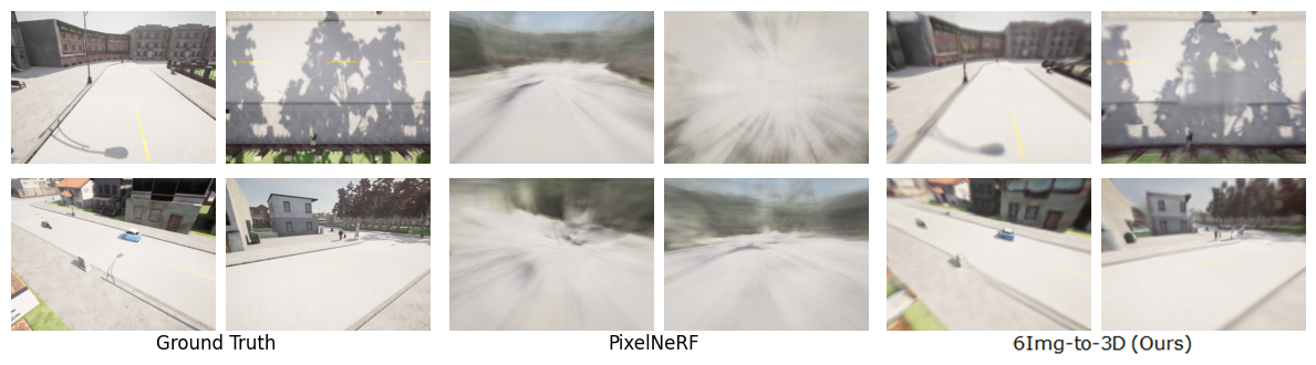
Figure 5: Visualization of the Comparison. PixelNeRF visibly struggles to reconstruct details and cannot resemble texture properly. Our method represents shape and appearance faithfully.

4.4 Ablation Study

Table 2: Ablation Results.

Method	PSNR $\uparrow$		SSIM $\uparrow$		LPIPS $\downarrow$
Sampling	Single	Double	Single	Double	Single	Double
w/o Scene Contraction	17.312	17.493	0.706	0.726	0.492	0.479
w/o $\mathcal{L}_{\text{LPIPS}}$	18.835	18.953	0.723	0.736	0.555	0.538
w/o Proj. Image Features	18.396	18.440	0.719	0.726	0.484	0.488
w    SwinFIR Upscaler${}^{\text{*}}$	-	19.188	-	0.746	-	0.444
6Img-to-3D (Ours)	18.762	18.864	0.719	0.733	0.453	0.453
* Not included in the full model since it visually impairs image quality.

We show the effectiveness of our model elements in Tab. 2 and visualize our ablations in Fig. 6. All model variants are trained for 100 epochs and evaluated on the holdout validation set consisting of 100 scenes from town two. We find that the scene contraction combined with the contracted cross-attention mechanism substantially improves the model performance. The PIFs and LPIPS help adjust the color values further. While LPIPS leads to more human-appealing images, this comes at the cost of reduced PSNR performance. Double and single sampling here refers to rendering the image with or without a more fine-grained second sampling step.

Additionally, an off-the-shelf upscaler, SwinFIR [107], is trained and tested on the output of our 6Img-to-3D model. While slightly improving on all metrics, a visual analysis shows that the upscaler only outputs a smoothed image instead of adding otherwise missing details.

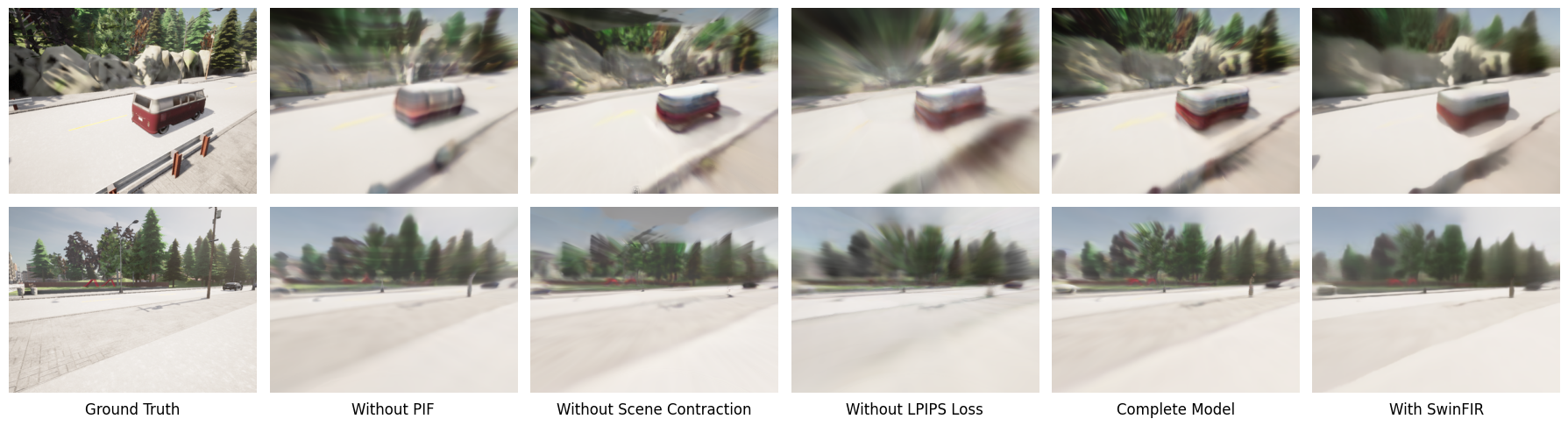
Figure 6: Visualization of the ablation. The final model particularly benefits from the LPIPS loss, the scene contraction, and the PIFs. When not using Scene Contraction, the out-of-bound objects are not rendered. Without the PIFs, the model struggles with fine details. Removing the LPIPS loss leads to increased smearing artifacts potentially caused by the projection of the PIFs along the camera rays.

4.5 Qualitative Results

Depth Values. We visualize the expected termination depth of each ray, resulting in the depth maps shown in Fig. 7. While never trained on depth information explicitly, 6Img-to-3D outputs reasonable depth maps.

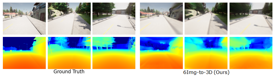
Figure 7: Depth Visualization. 6Img-to-3D infers a full 3D representation of the scene and can thus also be queried for density only, resulting in reasonable depth maps.

Consistency Over Timesteps. Our model works deterministically and thus obtains identical outputs for identical inputs. 6Img-to-3D also produces temporally consistent images across multiple consecutive timesteps without being explicitly trained to do so. A small change in the pose of the six input cameras results in a small change in the resulting output representation, visualized within the short trajectory in Fig. 8. When fed with six images per timestep, our model can also visualize longer scenes for example from a bird’s-eye view or a third-person perspective, see Fig. 8 long trajectory.

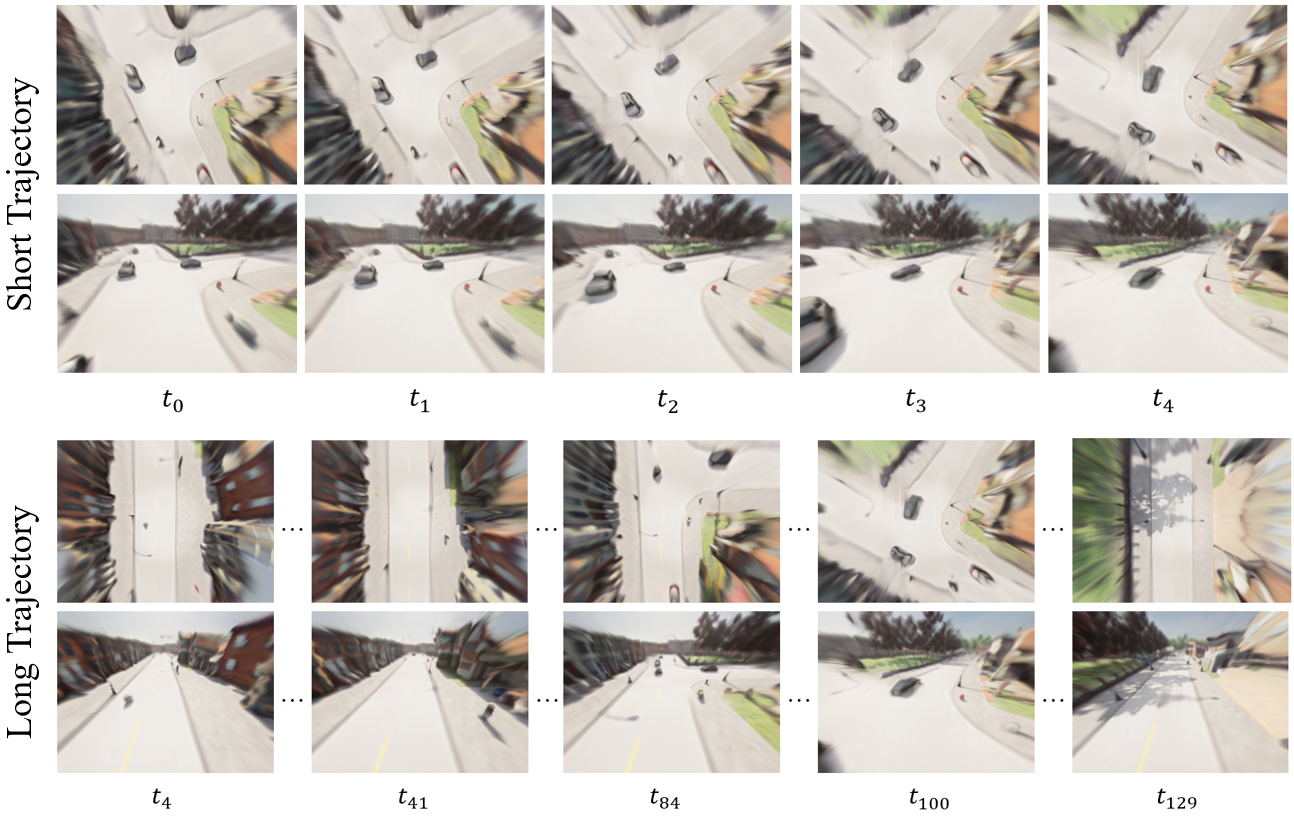
Figure 8: Trajectories. Consecutive timesteps are visualized with images from a BEV camera and behind and above the ego vehicle.

4.6 Effects of Scaling

Since our framework is self-supervised, we investigated whether our pipeline would benefit from a larger dataset. As shown in Fig. 9, the performance scales with the number of scenes.

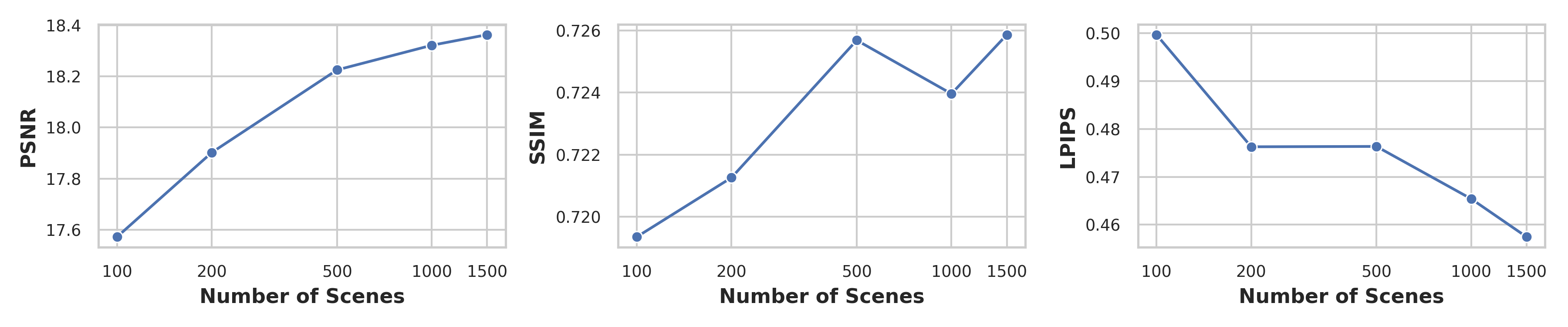
Figure 9: Effect of number of training scenes on performance.

5 Discussion

Conclusion. In this paper, we present 6Img-to-3D, an efficient and scalable method for reconstructing 3D representations of unbounded outdoor scenes from a few images. Our evaluation demonstrates that 6Img-to-3D can faithfully reconstruct third-person vehicle perspectives and birds-eye views using only six images with minimal overlap and without depth information. We achieve this by leveraging a triplanar representation of space, deformable attention mechanisms, feature projection and scene contraction. Our pipeline benefits from utilizing the features from the input images at multiple pipeline stages. A novel cross-attention sampling mechanism for contracted planes essentially drives performance gains. Our model could be further improved by additional training and using more data. We conclude this from the absence of overfitting during training and from how the model scales with data. An increased model size allows for a higher triplane resolution, which might help alleviate blurry texture for fine-grained details. Our model has around $\frac{1}{7}$ the amount of parameters of LRM [27], so visual fidelity could certainly be improved by scaling the model. We demonstrate the potential of our approach, particularly for embedded devices within vehicles, given its computational requirements. Seamless 2D-to-3D reconstruction could enhance driver assistance and autonomous driving systems, ultimately increasing road safety and navigation capabilities.

Future Directions. We see potential to improve the performance of our model. Initial experiments with an out-of-the-box upsampler trained on the data for post-rendering upscaling improved PSNR, SSIM, and LPIPS scores but introduced blurring (see Fig. 6). Incorporating the six source image information into the upscaling process represents a potentially valuable research direction to improve upscaling performance. The rendered could be extended to incorporate the viewing direction if incorporating view-dependent effects is required. This would allow the model to accurately recreate real-world materials, such as shiny metals or wet surfaces, with specular or glossy properties. We made some first attempts to run our trained model zero-shot on the nuScenes dataset [9]. Those zero-shot tests showed promising results that the model can be extended to real-world data. We assume that real-world driving data could be utilized by leveraging multi-timestep images for training. Using LiDAR for depth supervision or implementing a separate segmentation head would be natural extensions of our work.

Acknowledgements The research leading to these results is partially funded by the German Federal Ministry for Economic Affairs and Climate Action within the project “NXT GEN AI METHODS". The authors wish to extend their sincere gratitude to the creators of TPVformer, NeRFStudio, and the KPlanes paper for generously open-sourcing their code.

6 Appendix

6.1 Dataset Visualization

Table 3: Samples from Our Dataset. Towns differ in buildings (residential and commercial), types of bridges, amount of rivers, the traffic lights, and the kind of junctions. All towns contain pedestrians.

Town Input (Outward Facing) Supervision (Spherical Images) Town 1 Town 2 Town 3 Town 4 Town 5 Town 6

6.2 Bounded Scene Paramterization

The transformation from world coordinates $\bm{x_{W}}$ to grid coordinates $\bm{x_{grid}}$ can also be done when a bounded scene is given.

Bounded scenes: The world coordinates $\bm{x_{W}}$ are transformed into grid coordinates $\bm{x_{grid}}$ by scaling the scene with the scaling parameter $\bm{s}=[s_{h},s_{w},s_{z}]$ and applying the offset $\bm{o}=[o_{,}o_{w},o_{z}]$ according to Eq. 7 for element-wise operations. When depth maps are available, out-of-bound pixels of the training images can be masked with a white background during an initial testing phase, so the network learns only to reconstruct the inside of the bounded scene.

$$\bm{x_{grid}}=\frac{\bm{x_{W}}-\bm{o}}{\bm{s}}$$ (7)

6.3 Shape and Parameter Details

We follow the PyTorch convention of Batch $\times$ Channel $\times$ Height $\times$ Width ($B\times C\times H\times W$) in our description of the model. The shape of 6Img-to-3D is shown in Tab. 4.

Table 4: Shape and parameter values of 6Img-to-3D trained on the introduced dataset.

Part		Shape	Parameters
Input Images		$6\times 3\times 928\times 1600$	n.a.
ResNet Maps		$6\times 512\times 116\times 200$	44M
		$6\times 1024\times 58\times 100$
		$6\times 2048\times 29\times 50$
Feature Maps		$6\times 128\times 116\times 200$	1M
		$6\times 128\times 58\times 100$
		$6\times 128\times 29\times 50$
		$6\times 128\times 15\times 25$
Attention Mechanism		n.a.	16M
Triplane		$128\times 200\times 200$	n.a.
		$128\times 200\times 16$
		$128\times 16\times 200$
MLP decoder		input: 384	84K
		output: 4
Output Image		$3\times 600\times 800$

6.4 Zero-shot nuScenes Performance visualization

We attempt an early analysis of our 6Img-to-3D applied zero-shot to nuScenes. Without additional training, the model can display the appearance of nuscenes. Unfortunately, the camera setup within our dataset does not match the nuScenes data exactly. Camera positions, FOV, and scene style (sunny vs. cloudy weather) differ, making zero-shot transfer even more difficult. The promising results motivate to extent the model to real-world data.

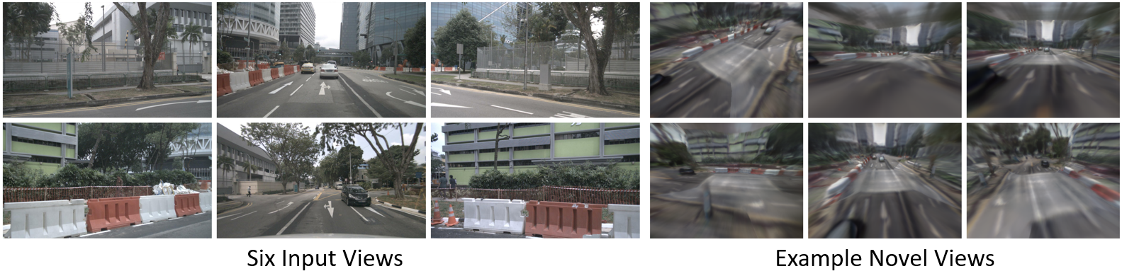
Figure 10: 6Img-to-3D with nuScenes Data.

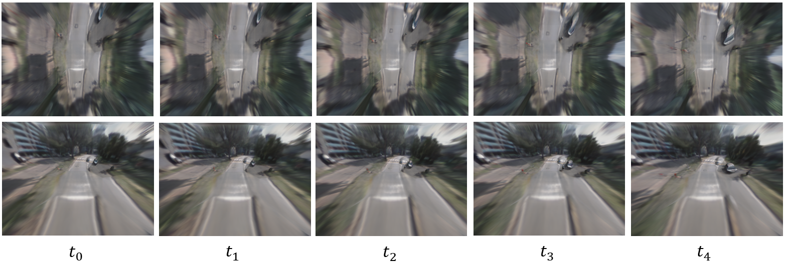
Figure 11: nuScenes Short Trajectory. Consecutive timesteps inferred during zero-shot inference on nuScenes.

6.5 Failure Cases

In Fig. 12, we visualize the failure cases of our method. Our model struggles with zero-shot reconstructing fine details, as seen in examples one and two. Partially, model failures can be attributed to the dataset itself. Some of the supervising images in the training set are located inside buildings. Within the Carla simulator, walls are sometimes transparent from within the building, which leads the model to pick up on this physically impossible artifact. Those failure cases are shown in examples three and four. Example five shows an instance where the model is unable to infer the structure of the building beyond what is actually contained in the input images.

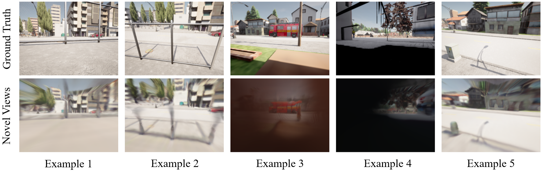
Figure 12: Visualization of Failure Cases.

6.6 Extended Qualitative Results Comparison

To give a better impression of our model’s performance, we here extend the visualization from our ablations. The results are not cherry-picked.

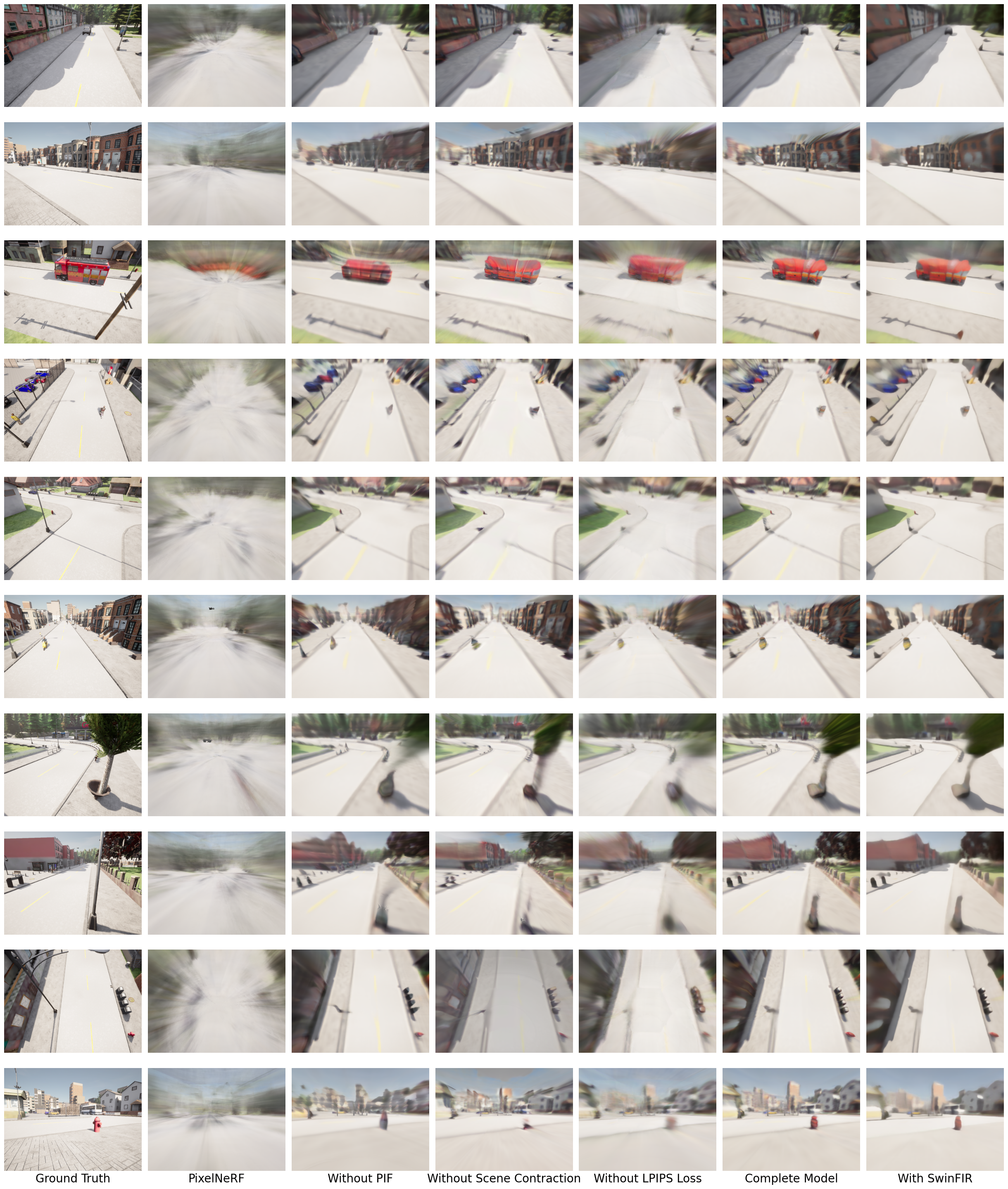
Figure 13: Qualitative Results Comparison (I).

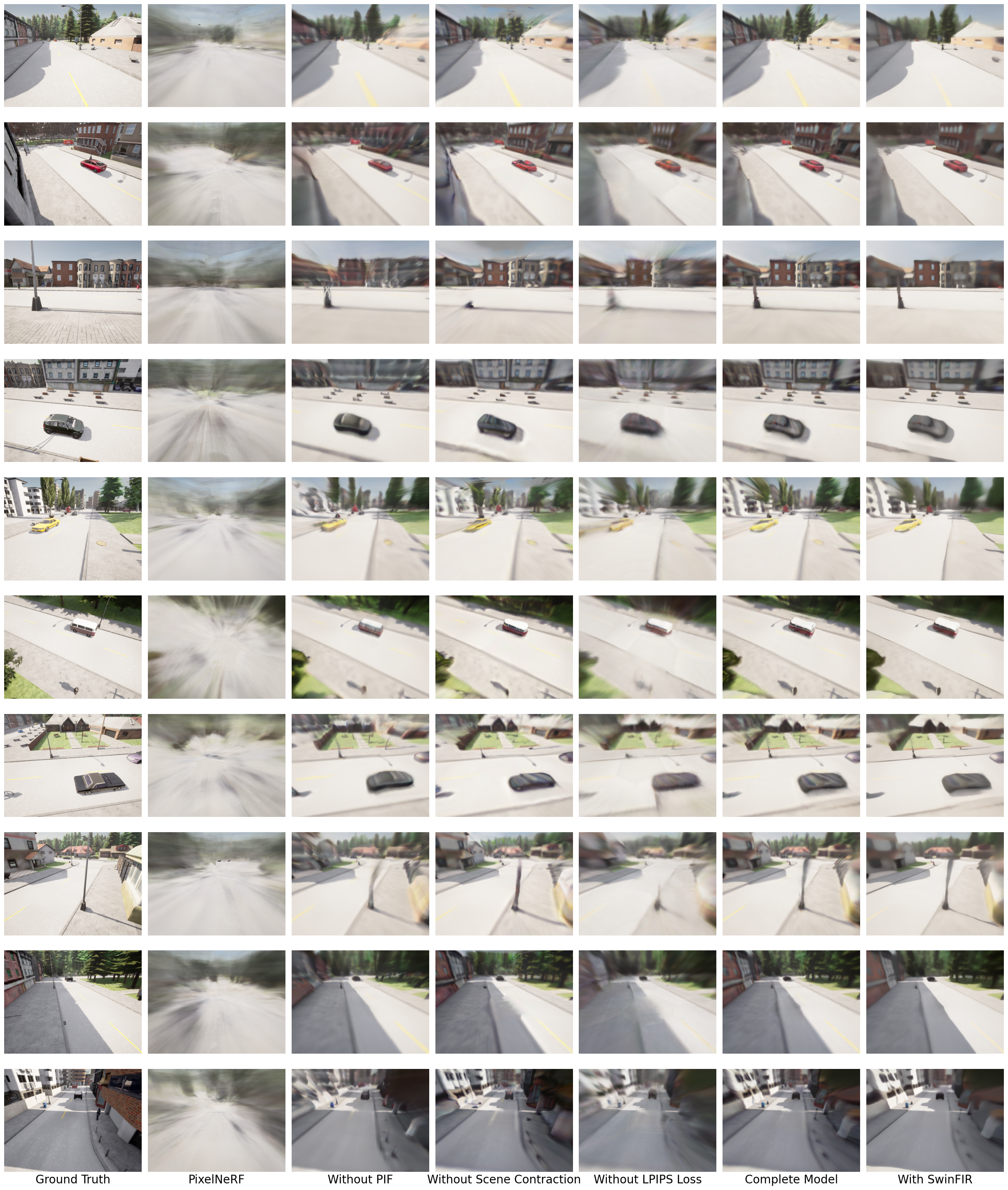
Figure 14: Qualitative Results Comparison (II).

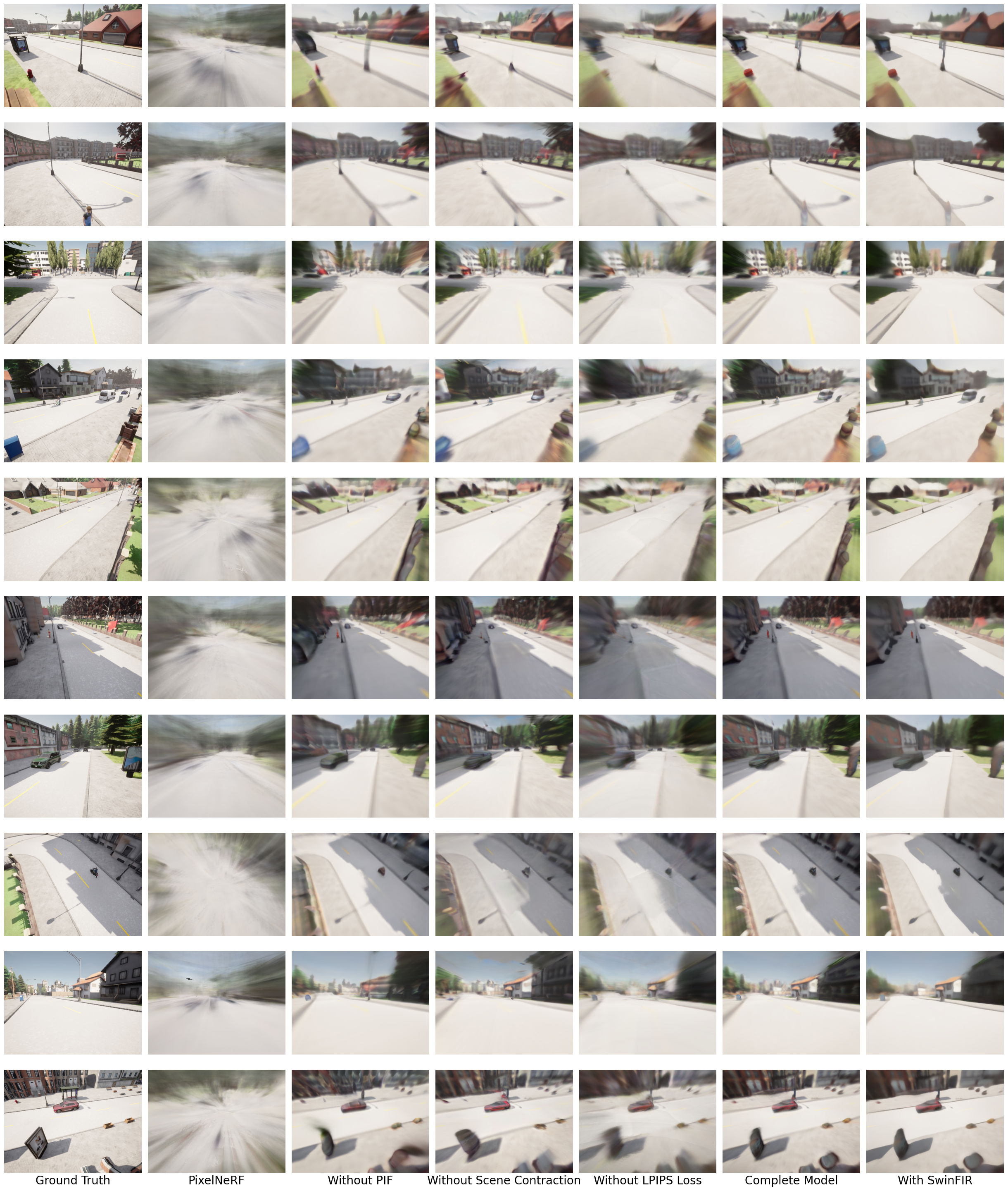
Figure 15: Qualitative Results Comparison (III).

References

- [1] Achlioptas, P., Diamanti, O., Mitliagkas, I., Guibas, L.: Learning representations and generative models for 3d point clouds (2018), arXiv:1707.02392
- [2] Adamkiewicz, M., Chen, T., Caccavale, A., Gardner, R., Culbertson, P., Bohg, J., Schwager, M.: Vision-only robot navigation in a neural radiance world (2022), arXiv:2110.00168
- [3] Anciukevicius, T., Xu, Z., Fisher, M., Henderson, P., Bilen, H., Mitra, N.J., Guerrero, P.: RenderDiffusion: Image Diffusion for 3D Reconstruction, Inpainting and Generation (Apr 2023), http://arxiv.org/abs/2211.09869, arXiv:2211.09869
- [4] Barron, J.T., Mildenhall, B., Verbin, D., Srinivasan, P.P., Hedman, P.: Mip-NeRF 360: Unbounded Anti-Aliased Neural Radiance Fields (Mar 2022), http://arxiv.org/abs/2111.12077, arXiv:2111.12077
- [5] Bautista, M.A., Guo, P., Abnar, S., Talbott, W., Toshev, A., Chen, Z., Dinh, L., Zhai, S., Goh, H., Ulbricht, D., Dehghan, A., Susskind, J.: GAUDI: A Neural Architect for Immersive 3D Scene Generation (Jul 2022), http://arxiv.org/abs/2207.13751, arXiv:2207.13751
- [6] Behley, J., Garbade, M., Milioto, A., Quenzel, J., Behnke, S., Stachniss, C., Gall, J.: SemanticKITTI: A Dataset for Semantic Scene Understanding of LiDAR Sequences (Aug 2019), http://arxiv.org/abs/1904.01416, arXiv:1904.01416
- [7] Bhattarai, A.R., Nießner, M., Sevastopolsky, A.: TriPlaneNet: An Encoder for EG3D Inversion (Mar 2023), http://arxiv.org/abs/2303.13497, arXiv:2303.13497
- [8] Bogdoll, D., Yang, Y., Zöllner, J.M.: Muvo: A multimodal generative world model for autonomous driving with geometric representations (2023), arXiv:2311.11762
- [9] Caesar, H., Bankiti, V., Lang, A.H., Vora, S., Liong, V.E., Xu, Q., Krishnan, A., Pan, Y., Baldan, G., Beijbom, O.: nuScenes: A multimodal dataset for autonomous driving (May 2020), http://arxiv.org/abs/1903.11027, arXiv:1903.11027
- [10] Chai, L., Tucker, R., Li, Z., Isola, P., Snavely, N.: Persistent nature: A generative model of unbounded 3d worlds (2023), arXiv:2303.13515
- [11] Chan, E.R., Lin, C.Z., Chan, M.A., Nagano, K., Pan, B., De Mello, S., Gallo, O., Guibas, L., Tremblay, J., Khamis, S., Karras, T., Wetzstein, G.: Efficient Geometry-aware 3D Generative Adversarial Networks (Apr 2022), http://arxiv.org/abs/2112.07945, arXiv:2112.07945
- [12] Charatan, D., Li, S., Tagliasacchi, A., Sitzmann, V.: pixelsplat: 3d gaussian splats from image pairs for scalable generalizable 3d reconstruction (2023), arXiv:2312.12337
- [13] Chen, A., Xu, Z., Geiger, A., Yu, J., Su, H.: TensoRF: Tensorial Radiance Fields (Nov 2022), http://arxiv.org/abs/2203.09517, arXiv:2203.09517
- [14] Chen, A., Xu, Z., Zhao, F., Zhang, X., Xiang, F., Yu, J., Su, H.: Mvsnerf: Fast generalizable radiance field reconstruction from multi-view stereo (2021), arXiv:2103.15595
- [15] Chen, L., Wu, P., Chitta, K., Jaeger, B., Geiger, A., Li, H.: End-to-end autonomous driving: Challenges and frontiers (2023), arXiv:2306.16927
- [16] Chen, Z., Wang, G., Liu, Z.: Scenedreamer: Unbounded 3d scene generation from 2d image collections. IEEE Transactions on Pattern Analysis and Machine Intelligence 45(12), 15562–15576 (Dec 2023). https://doi.org/10.1109/tpami.2023.3321857, http://dx.doi.org/10.1109/TPAMI.2023.3321857
- [17] Chen, Z., Zhang, H.: Learning implicit fields for generative shape modeling (2019), arXiv:1812.02822
- [18] Deng, C., Jiang, C.M., Qi, C.R., Yan, X., Zhou, Y., Guibas, L., Anguelov, D.: Nerdi: Single-view nerf synthesis with language-guided diffusion as general image priors (2022), arXiv:2212.03267
- [19] Dosovitskiy, A., Ros, G., Codevilla, F., Lopez, A., Koltun, V.: Carla: An open urban driving simulator (2017), arXiv:1711.03938
- [20] Fan, H., Su, H., Guibas, L.: A point set generation network for 3d object reconstruction from a single image (2016), arXiv:1612.00603
- [21] Fridovich-Keil, S., Meanti, G., Warburg, F., Recht, B., Kanazawa, A.: K-Planes: Explicit Radiance Fields in Space, Time, and Appearance (Mar 2023), http://arxiv.org/abs/2301.10241, arXiv:2301.10241
- [22] Gao, J., Shen, T., Wang, Z., Chen, W., Yin, K., Li, D., Litany, O., Gojcic, Z., Fidler, S.: GET3D: A Generative Model of High Quality 3D Textured Shapes Learned from Images (Sep 2022), http://arxiv.org/abs/2209.11163, arXiv:2209.11163
- [23] Gao, K., Gao, Y., He, H., Lu, D., Xu, L., Li, J.: Nerf: Neural radiance field in 3d vision, a comprehensive review (2023), arXiv:2210.00379
- [24] Girdhar, R., Fouhey, D.F., Rodriguez, M., Gupta, A.: Learning a predictable and generative vector representation for objects (2016), arXiv:1603.08637
- [25] Gu, J., Trevithick, A., Lin, K.E., Susskind, J., Theobalt, C., Liu, L., Ramamoorthi, R.: NerfDiff: Single-image View Synthesis with NeRF-guided Distillation from 3D-aware Diffusion (Feb 2023), http://arxiv.org/abs/2302.10109, arXiv:2302.10109
- [26] He, K., Zhang, X., Ren, S., Sun, J.: Deep residual learning for image recognition (2015), arXiv:1512.03385
- [27] Hong, Y., Zhang, K., Gu, J., Bi, S., Zhou, Y., Liu, D., Liu, F., Sunkavalli, K., Bui, T., Tan, H.: Lrm: Large reconstruction model for single image to 3d (2023), arXiv:2311.04400
- [28] Huang, Y., Zheng, W., Zhang, Y., Zhou, J., Lu, J.: Tri-perspective view for vision-based 3d semantic occupancy prediction (2023), arXiv:2302.07817
- [29] Huang, Y., Zheng, W., Zhang, Y., Zhou, J., Lu, J.: Tri-Perspective View for Vision-Based 3D Semantic Occupancy Prediction (Mar 2023), http://arxiv.org/abs/2302.07817, arXiv:2302.07817
- [30] Irshad, M.Z., Zakharov, S., Liu, K., Guizilini, V., Kollar, T., Gaidon, A., Kira, Z., Ambrus, R.: NeO 360: Neural Fields for Sparse View Synthesis of Outdoor Scenes (Aug 2023), http://arxiv.org/abs/2308.12967, arXiv:2308.12967
- [31] Johari, M.M., Lepoittevin, Y., Fleuret, F.: Geonerf: Generalizing nerf with geometry priors (2022), arXiv:2111.13539
- [32] Kanazawa, A., Tulsiani, S., Efros, A.A., Malik, J.: Learning category-specific mesh reconstruction from image collections (2018), arXiv:1803.07549
- [33] Kim, S.W., Brown, B., Yin, K., Kreis, K., Schwarz, K., Li, D., Rombach, R., Torralba, A., Fidler, S.: Neuralfield-ldm: Scene generation with hierarchical latent diffusion models (2023), arXiv:2304.09787
- [34] Kingma, D.P., Ba, J.: Adam: A method for stochastic optimization (2017), arXiv:1412.6980
- [35] Koh, J.Y., Lee, H., Yang, Y., Baldridge, J., Anderson, P.: Pathdreamer: A world model for indoor navigation (2021), arXiv:2105.08756
- [36] Li, Z., Wang, Q., Snavely, N., Kanazawa, A.: Infinitenature-zero: Learning perpetual view generation of natural scenes from single images (2022), arXiv:2207.11148
- [37] Li, Z., Wang, W., Li, H., Xie, E., Sima, C., Lu, T., Yu, Q., Dai, J.: BEVFormer: Learning Bird’s-Eye-View Representation from Multi-Camera Images via Spatiotemporal Transformers (Jul 2022), http://arxiv.org/abs/2203.17270, arXiv:2203.17270
- [38] Liang, R., Zhang, J., Li, H., Yang, C., Guan, Y., Vijaykumar, N.: Spidr: Sdf-based neural point fields for illumination and deformation (2023), arXiv:2210.08398
- [39] Lin, C.H., Lee, H.Y., Menapace, W., Chai, M., Siarohin, A., Yang, M.H., Tulyakov, S.: Infinicity: Infinite-scale city synthesis (2023), arXiv:2301.09637
- [40] Lin, K.E., Yen-Chen, L., Lai, W.S., Lin, T.Y., Shih, Y.C., Ramamoorthi, R.: Vision Transformer for NeRF-Based View Synthesis from a Single Input Image (Oct 2022), http://arxiv.org/abs/2207.05736, arXiv:2207.05736
- [41] Lin, T.Y., Dollár, P., Girshick, R., He, K., Hariharan, B., Belongie, S.: Feature pyramid networks for object detection (2017), arXiv:1612.03144
- [42] Lin, Y., Han, H., Gong, C., Xu, Z., Zhang, Y., Li, X.: Consistent123: One image to highly consistent 3d asset using case-aware diffusion priors (2023), arXiv:2309.17261
- [43] Liu, A., Tucker, R., Jampani, V., Makadia, A., Snavely, N., Kanazawa, A.: Infinite nature: Perpetual view generation of natural scenes from a single image (2021), arXiv:2012.09855
- [44] Liu, L., Gu, J., Lin, K.Z., Chua, T.S., Theobalt, C.: Neural sparse voxel fields (2021), arXiv:2007.11571
- [45] Liu, M., Xu, C., Jin, H., Chen, L., T, M.V., Xu, Z., Su, H.: One-2-3-45: Any single image to 3d mesh in 45 seconds without per-shape optimization (2023), arXiv:2306.16928
- [46] Liu, R., Wu, R., Hoorick, B.V., Tokmakov, P., Zakharov, S., Vondrick, C.: Zero-1-to-3: Zero-shot one image to 3d object (2023), arXiv:2303.11328
- [47] Liu, Y., Peng, S., Liu, L., Wang, Q., Wang, P., Theobalt, C., Zhou, X., Wang, W.: Neural rays for occlusion-aware image-based rendering (2022), arXiv:2107.13421
- [48] Liu, Z., Feng, Y., Black, M.J., Nowrouzezahrai, D., Paull, L., Liu, W.: Meshdiffusion: Score-based generative 3d mesh modeling (2023), arXiv:2303.08133
- [49] Lombardi, S., Simon, T., Saragih, J., Schwartz, G., Lehrmann, A., Sheikh, Y.: Neural volumes: learning dynamic renderable volumes from images. ACM Transactions on Graphics 38(4), 1–14 (Jul 2019). https://doi.org/10.1145/3306346.3323020, http://dx.doi.org/10.1145/3306346.3323020
- [50] Loshchilov, I., Hutter, F.: Sgdr: Stochastic gradient descent with warm restarts (2017), arXiv:1608.03983
- [51] Maggio, D., Abate, M., Shi, J., Mario, C., Carlone, L.: Loc-nerf: Monte carlo localization using neural radiance fields (2022), arXiv:2209.09050
- [52] Max, N.: Optical models for direct volume rendering. IEEE Transactions on Visualization and Computer Graphics 1(2), 99–108 (jun 1995). https://doi.org/10.1109/2945.468400, https://doi.org/10.1109/2945.468400
- [53] Melas-Kyriazi, L., Rupprecht, C., Laina, I., Vedaldi, A.: Realfusion: 360 reconstruction of any object from a single image (2023), arXiv:2302.10663
- [54] Mildenhall, B., Srinivasan, P.P., Tancik, M., Barron, J.T., Ramamoorthi, R., Ng, R.: Synthetic nerf dataset, https://drive.google.com/drive/folders/128yBriW1IG_3NJ5Rp7APSTZsJqdJdfc1
- [55] Mildenhall, B., Srinivasan, P.P., Tancik, M., Barron, J.T., Ramamoorthi, R., Ng, R.: NeRF: Representing Scenes as Neural Radiance Fields for View Synthesis (Aug 2020), http://arxiv.org/abs/2003.08934, arXiv:2003.08934
- [56] Müller, T., Evans, A., Schied, C., Keller, A.: Instant neural graphics primitives with a multiresolution hash encoding. ACM Transactions on Graphics 41(4), 1–15 (Jul 2022). https://doi.org/10.1145/3528223.3530127, https://dl.acm.org/doi/10.1145/3528223.3530127
- [57] Nash, C., Ganin, Y., Eslami, S.M.A., Battaglia, P.W.: Polygen: An autoregressive generative model of 3d meshes (2020), arXiv:2002.10880
- [58] Niemeyer, M., Barron, J.T., Mildenhall, B., Sajjadi, M.S.M., Geiger, A., Radwan, N.: RegNeRF: Regularizing Neural Radiance Fields for View Synthesis from Sparse Inputs (Dec 2021), http://arxiv.org/abs/2112.00724, arXiv:2112.00724
- [59] Niemeyer, M., Mescheder, L., Oechsle, M., Geiger, A.: Differentiable volumetric rendering: Learning implicit 3d representations without 3d supervision (2020), arXiv:1912.07372
- [60] Ortiz, J., Clegg, A., Dong, J., Sucar, E., Novotny, D., Zollhoefer, M., Mukadam, M.: isdf: Real-time neural signed distance fields for robot perception (2022), arXiv:2204.02296
- [61] Ost, J., Mannan, F., Thuerey, N., Knodt, J., Heide, F.: Neural scene graphs for dynamic scenes (2021), arXiv:2011.10379
- [62] Po, R., Yifan, W., Golyanik, V., Aberman, K., Barron, J.T., Bermano, A.H., Chan, E.R., Dekel, T., Holynski, A., Kanazawa, A., Liu, C.K., Liu, L., Mildenhall, B., Nießner, M., Ommer, B., Theobalt, C., Wonka, P., Wetzstein, G.: State of the art on diffusion models for visual computing (2023), arXiv:2310.07204
- [63] Raj, A., Kaza, S., Poole, B., Niemeyer, M., Ruiz, N., Mildenhall, B., Zada, S., Aberman, K., Rubinstein, M., Barron, J., Li, Y., Jampani, V.: Dreambooth3d: Subject-driven text-to-3d generation (2023), arXiv:2303.13508
- [64] Rebain, D., Jiang, W., Yazdani, S., Li, K., Yi, K.M., Tagliasacchi, A.: DeRF: Decomposed Radiance Fields (Nov 2020), http://arxiv.org/abs/2011.12490, arXiv:2011.12490
- [65] Reiher, L., Lampe, B., Eckstein, L.: A Sim2Real Deep Learning Approach for the Transformation of Images from Multiple Vehicle-Mounted Cameras to a Semantically Segmented Image in Bird’s Eye View (May 2020), http://arxiv.org/abs/2005.04078, arXiv:2005.04078
- [66] Reiser, C., Peng, S., Liao, Y., Geiger, A.: KiloNeRF: Speeding up Neural Radiance Fields with Thousands of Tiny MLPs (Aug 2021), http://arxiv.org/abs/2103.13744, arXiv:2103.13744
- [67] Ren, Y., Wang, F., Zhang, T., Pollefeys, M., Süsstrunk, S.: VolRecon: Volume Rendering of Signed Ray Distance Functions for Generalizable Multi-View Reconstruction (Apr 2023), http://arxiv.org/abs/2212.08067, arXiv:2212.08067
- [68] Seitz, S.M., Dyer, C.R.: Photorealistic scene reconstruction by voxel coloring. In: Proceedings of the 1997 Conference on Computer Vision and Pattern Recognition (CVPR ’97). p. 1067. CVPR ’97, IEEE Computer Society, USA (1997)
- [69] Seo, J., Jang, W., Kwak, M.S., Ko, J., Kim, H., Kim, J., Kim, J.H., Lee, J., Kim, S.: Let 2d diffusion model know 3d-consistency for robust text-to-3d generation (2023), arXiv:2303.07937
- [70] Sharma, P., Tewari, A., Du, Y., Zakharov, S., Ambrus, R., Gaidon, A., Freeman, W.T., Durand, F., Tenenbaum, J.B., Sitzmann, V.: Neural groundplans: Persistent neural scene representations from a single image (2023), arXiv:2207.11232
- [71] Shue, J.R., Chan, E.R., Po, R., Ankner, Z., Wu, J., Wetzstein, G.: 3D Neural Field Generation using Triplane Diffusion (Nov 2022), http://arxiv.org/abs/2211.16677, arXiv:2211.16677
- [72] Sima, C., Tong, W., Wang, T., Chen, L., Wu, S., Deng, H., Gu, Y., Lu, L., Luo, P., Lin, D., Li, H.: Scene as occupancy (2023), arXiv:2306.02851
- [73] Sun, C., Sun, M., Chen, H.T.: Direct Voxel Grid Optimization: Super-fast Convergence for Radiance Fields Reconstruction. In: 2022 IEEE/CVF Conference on Computer Vision and Pattern Recognition (CVPR). pp. 5449–5459. IEEE, New Orleans, LA, USA (Jun 2022). https://doi.org/10.1109/CVPR52688.2022.00538, https://ieeexplore.ieee.org/document/9879963/
- [74] Sun, P., Kretzschmar, H., Dotiwalla, X., Chouard, A., Patnaik, V., Tsui, P., Guo, J., Zhou, Y., Chai, Y., Caine, B., Vasudevan, V., Han, W., Ngiam, J., Zhao, H., Timofeev, A., Ettinger, S., Krivokon, M., Gao, A., Joshi, A., Zhang, Y., Shlens, J., Chen, Z., Anguelov, D.: Scalability in perception for autonomous driving: Waymo open dataset. In: Proceedings of the IEEE/CVF Conference on Computer Vision and Pattern Recognition (CVPR) (June 2020)
- [75] Szeliski, R.: Computer Vision: Algorithms and Applications. Springer-Verlag, Berlin, Heidelberg, 1st edn. (2010)
- [76] Szymanowicz, S., Rupprecht, C., Vedaldi, A.: Splatter image: Ultra-fast single-view 3d reconstruction (2023), arXiv:2312.13150
- [77] Tagliasacchi, A., Mildenhall, B.: Volume rendering digest (for nerf) (2022), arXiv:2209.02417
- [78] Tancik, M., Casser, V., Yan, X., Pradhan, S., Mildenhall, B., Srinivasan, P.P., Barron, J.T., Kretzschmar, H.: Block-NeRF: Scalable Large Scene Neural View Synthesis (Feb 2022), http://arxiv.org/abs/2202.05263, arXiv:2202.05263
- [79] Tewari, A., Thies, J., Mildenhall, B., Srinivasan, P., Tretschk, E., Yifan, W., Lassner, C., Sitzmann, V., Martin-Brualla, R., Lombardi, S., Simon, T., Theobalt, C., Nießner, M., Barron, J.T., Wetzstein, G., Zollhöfer, M., Golyanik, V.: Advances in Neural Rendering. Computer Graphics Forum (EG STAR 2022) (2022)
- [80] Thrun, S., Burgard, W., Fox, D.: Probabilistic Robotics (Intelligent Robotics and Autonomous Agents). The MIT Press (2005)
- [81] Tian, X., Jiang, T., Yun, L., Mao, Y., Yang, H., Wang, Y., Wang, Y., Zhao, H.: Occ3d: A large-scale 3d occupancy prediction benchmark for autonomous driving (2023), arXiv:2304.14365
- [82] Trevithick, A., Yang, B.: Grf: Learning a general radiance field for 3d representation and rendering (2021), arXiv:2010.04595
- [83] Wang, N., Zhang, Y., Li, Z., Fu, Y., Liu, W., Jiang, Y.G.: Pixel2mesh: Generating 3d mesh models from single rgb images (2018), arXiv:1804.01654
- [84] Wang, P., Liu, L., Liu, Y., Theobalt, C., Komura, T., Wang, W.: Neus: Learning neural implicit surfaces by volume rendering for multi-view reconstruction. NeurIPS (2021)
- [85] Wang, Q., Wang, Z., Genova, K., Srinivasan, P., Zhou, H., Barron, J.T., Martin-Brualla, R., Snavely, N., Funkhouser, T.: IBRNet: Learning Multi-View Image-Based Rendering (Apr 2021), http://arxiv.org/abs/2102.13090, arXiv:2102.13090
- [86] Watson, D., Chan, W., Martin-Brualla, R., Ho, J., Tagliasacchi, A., Norouzi, M.: Novel View Synthesis with Diffusion Models (Oct 2022), http://arxiv.org/abs/2210.04628, arXiv:2210.04628
- [87] Wei, Y., Zhao, L., Zheng, W., Zhu, Z., Zhou, J., Lu, J.: Surroundocc: Multi-camera 3d occupancy prediction for autonomous driving (2023), arXiv:2303.09551
- [88] Wu, J., Wang, Y., Xue, T., Sun, X., Freeman, W.T., Tenenbaum, J.B.: Marrnet: 3d shape reconstruction via 2.5d sketches (2017), arXiv:1711.03129
- [89] Wu, P., Escontrela, A., Hafner, D., Goldberg, K., Abbeel, P.: Daydreamer: World models for physical robot learning (2022), arXiv:2206.14176
- [90] Xie, H., Chen, Z., Hong, F., Liu, Z.: Citydreamer: Compositional generative model of unbounded 3d cities (2023), arXiv:2309.00610
- [91] Xie, H., Yao, H., Zhang, S., Zhou, S., Sun, W.: Pix2vox++: Multi-scale context-aware 3d object reconstruction from single and multiple images. International Journal of Computer Vision 128(12), 2919–2935 (Jul 2020). https://doi.org/10.1007/s11263-020-01347-6, http://dx.doi.org/10.1007/s11263-020-01347-6
- [92] Xie, Y., Takikawa, T., Saito, S., Litany, O., Yan, S., Khan, N., Tombari, F., Tompkin, J., Sitzmann, V., Sridhar, S.: Neural fields in visual computing and beyond (2022), arXiv:2111.11426
- [93] Xu, D., Jiang, Y., Wang, P., Fan, Z., Wang, Y., Wang, Z.: Neurallift-360: Lifting an in-the-wild 2d photo to a 3d object with 360 views (2023), arXiv:2211.16431
- [94] Xu, Q., Wang, W., Ceylan, D., Mech, R., Neumann, U.: Disn: Deep implicit surface network for high-quality single-view 3d reconstruction (2021), arXiv:1905.10711
- [95] Xu, Y., Chai, M., Shi, Z., Peng, S., Skorokhodov, I., Siarohin, A., Yang, C., Shen, Y., Lee, H.Y., Zhou, B., Tulyakov, S.: Discoscene: Spatially disentangled generative radiance fields for controllable 3d-aware scene synthesis (2022), arXiv:2212.11984
- [96] Xu, Y., Tan, H., Luan, F., Bi, S., Wang, P., Li, J., Shi, Z., Sunkavalli, K., Wetzstein, G., Xu, Z., Zhang, K.: Dmv3d: Denoising multi-view diffusion using 3d large reconstruction model (2023), arXiv:2311.09217
- [97] Yagubbayli, F., Wang, Y., Tonioni, A., Tombari, F.: Legoformer: Transformers for block-by-block multi-view 3d reconstruction (2022), arXiv:2106.12102
- [98] Yang, J., Pavone, M., Wang, Y.: Freenerf: Improving few-shot neural rendering with free frequency regularization (2023), arXiv:2303.07418
- [99] Yang, W., Li, Q., Liu, W., Yu, Y., Ma, Y., He, S., Pan, J.: Projecting Your View Attentively: Monocular Road Scene Layout Estimation via Cross-view Transformation. In: 2021 IEEE/CVF Conference on Computer Vision and Pattern Recognition (CVPR). pp. 15531–15540. IEEE, Nashville, TN, USA (Jun 2021). https://doi.org/10.1109/CVPR46437.2021.01528, https://ieeexplore.ieee.org/document/9578824/
- [100] Yang, Y., Feng, C., Shen, Y., Tian, D.: Foldingnet: Point cloud auto-encoder via deep grid deformation (2018), arXiv:1712.07262
- [101] Yu, A., Fridovich-Keil, S., Tancik, M., Chen, Q., Recht, B., Kanazawa, A.: Plenoxels: Radiance Fields without Neural Networks (Dec 2021), http://arxiv.org/abs/2112.05131, arXiv:2112.05131
- [102] Yu, A., Li, R., Tancik, M., Li, H., Ng, R., Kanazawa, A.: PlenOctrees for Real-time Rendering of Neural Radiance Fields. In: 2021 IEEE/CVF International Conference on Computer Vision (ICCV). pp. 5732–5741. IEEE, Montreal, QC, Canada (Oct 2021). https://doi.org/10.1109/ICCV48922.2021.00570, https://ieeexplore.ieee.org/document/9711398/
- [103] Yu, A., Ye, V., Tancik, M., Kanazawa, A.: pixelnerf: Neural radiance fields from one or few images (2021), arXiv:2012.02190
- [104] Yu, A., Ye, V., Tancik, M., Kanazawa, A.: pixelNeRF: Neural Radiance Fields from One or Few Images (May 2021), http://arxiv.org/abs/2012.02190, arXiv:2012.02190
- [105] Yu, X., Rao, Y., Wang, Z., Liu, Z., Lu, J., Zhou, J.: Pointr: Diverse point cloud completion with geometry-aware transformers (2021), arXiv:2108.08839
- [106] Zeng, X., Vahdat, A., Williams, F., Gojcic, Z., Litany, O., Fidler, S., Kreis, K.: Lion: Latent point diffusion models for 3d shape generation (2022), arXiv:2210.06978
- [107] Zhang, D., Huang, F., Liu, S., Wang, X., Jin, Z.: Swinfir: Revisiting the swinir with fast fourier convolution and improved training for image super-resolution (2023), arXiv:2208.11247
- [108] Zhang, K., Riegler, G., Snavely, N., Koltun, V.: NeRF++: Analyzing and Improving Neural Radiance Fields (Oct 2020), http://arxiv.org/abs/2010.07492, arXiv:2010.07492
- [109] Zhang, K., Riegler, G., Snavely, N., Koltun, V.: Nerf++: Analyzing and improving neural radiance fields (2020), arXiv:2010.07492
- [110] Zhang, R., Isola, P., Efros, A.A., Shechtman, E., Wang, O.: The unreasonable effectiveness of deep features as a perceptual metric (2018), arXiv:1801.03924
- [111] Zheng, W., Chen, W., Huang, Y., Zhang, B., Duan, Y., Lu, J.: Occworld: Learning a 3d occupancy world model for autonomous driving (2023), arXiv:2311.16038
- [112] Zhu, X., Su, W., Lu, L., Li, B., Wang, X., Dai, J.: Deformable DETR: Deformable Transformers for End-to-End Object Detection (Mar 2021), http://arxiv.org/abs/2010.04159, arXiv:2010.04159