Entanglement generation between two comoving Unruh-DeWitt detectors in the cosmological de Sitter spacetime

Abstract

We investigate the entanglement generation or harvesting between two identical Unruh-DeWitt detectors in the cosmological de Sitter spacetime. We consider two comoving two-level detectors at a coincident spatial position. The detectors are assumed to be unentangled initially. The detectors are individually coupled to a scalar field, which eventually leads to coupling between the two detectors. We consider two kinds of scalar fields – conformally symmetric and massless minimally coupled, for both real and complex cases. By tracing out the degrees of freedom corresponding to the scalar field, we construct the reduced density matrix for the two detectors, whose eigenvalues characterise transitions between the energy levels of the detectors. By using the existing results for the detector response functions per unit proper time for these fields, we next compute the logarithmic negativity, quantifying the degree of entanglement generated at late times between the two detectors. The similarities and differences of these results for different kind of scalar fields have been discussed.

I Introduction

The phenomenon of quantum entanglement is even more counter intuitive compared to the standard quantum mechanical processes. Experimental observations, for example, of the violation of the Bell inequalities, which cannot be explained by classical theories based upon local hidden variables, have placed quantum entanglement on very strong physical grounds bell_1 ; bell_2 ; bell_3 ; bell_4 . One of the defining characteristics of entangled states is the inability to describe the corresponding Hilbert space as a product of pure states of subsystems, e.g. NielsenChuang and references therein. In addition to its foundational role in quantum physics, quantum entanglement has found a wide range of applications in the modern world, from building high-security communication systems by employing quantum cryptography to futuristic quantum teleportation based devices, e.g. WJHN ; DAC ; Hotta:2008uk ; MKM .

Recently, the research community has also shown considerable interest in studying quantum entanglement in the context of relativistic quantum field theory Reznik:2002fz ; Martin-Martinez:2015qwa ; Fuentes:2010dt ; Anastopoulos:2022owu ; Casini:2022rlv ; Preskill ; RevModPhys ; Jordan:2011ci ; Giddings:2012bm ; Calabrese:2004eu ; Wu:2022glj . An essential focus of this is to examine the dynamics of quantum particles coupled to a quantum field, particularly using particle detectors. These investigations encompass studying entanglement dynamics, entanglement harvesting, and understanding the radiative processes of entangled relativistic particles Menezes:2015veo ; Menezes:2015iva ; Iso:2016lua ; Lindel:2023rfi ; Lima:2023pyt ; Elghaayda:2023igv ; Barman:2022xht ; Kaushal:2022las . Entanglement harvesting, in particular, is intriguing as it offers a means to extract additional quantum information.

The Unruh-DeWitt detectors are very popular in the context of relativistic quantum entanglement. Initially designed for studying Unruh radiation observed by a uniformly accelerated observer in the Minkowski spacetime, they were also used for studyig Hawking radiation in eternal black hole spacetimes Unruh . In this paper, we wish to examine the conditions under which these detectors become entangled over time in the presence of a coupling with a quantum field. such framework allows us to explore the potential for entanglement harvesting between initially uncorrelated detectors. Various earlier investigations show different factors could contribute to this detector entanglement, including detectors’ trajectories Reznik:2002fz ; Benatti:2004ee ; Salton:2014jaa ; Koga:2018the ; Koga:2019fqh ; Zhang:2020xvo , the background spacetime geometry Fuentes-Schuller:2004iaz ; Henderson:2017yuv ; Wu:2023glc ; Martin-Martinez:2012chf ; Tjoa:2022oxv ; Bhattacharya:2022ahn ; Dhanuka:2022ggi ; Maeso-Garcia:2022uzf ; Martin-Martinez:2015eoa ; Mendez-Avalos:2022obb ; Perche:2022ykt , the presence of a thermal bath Brown:2013kia ; Barman:2021kwg ; Henderson:2022oyd , and even the transient passage of gravitational waves Prokopec:2022akz ; Xu:2020pbj .

In particular, a large number of works have actively engaged in understanding the entanglement harvesting patterns of Unruh-DeWitt detectors that interact perturbatively with quantum fields. These works span from inertial detectors in flat spacetime Barman:2022xht ; Barman:2021kwg ; Koga:2018the ; Koga:2019fqh to those following various trajectories in curved spacetime Fuentes-Schuller:2004iaz ; Martin-Martinez:2015qwa ; Fuentes:2010dt ; Henderson:2017yuv ; Robbins:2020jca ; Cong:2020nec ; Gallock-Yoshimura:2021yok . For various such studies, we further refer our reader to Reznik:2002fz ; Benatti:2004ee ; Salton:2014jaa ; Zhang:2020xvo ; Brown:2013kia ; Henderson:2022oyd ; Pozas-Kerstjens:2015gta ; Xu:2020pbj ; Cliche:2010fi (also references therein). See Chowdhury:2021ieg ; Barman:2022loh for study of degradation/entanglement generation between two initially correlated Unruh-DeWitt detectors. See also Makarov:2017erw ; Brown:2012pw for discussion on some non-perturbative effects. We note that studying such features of entanglement in the early inflationary background can provide valuable insights about the geometry as well as the quantum condition at such stage. For instance, entanglement generated in the early universe could affect cosmological correlation functions or the cosmic microwave background Boyanovsky:2018soy ; Rauch:2018rvx ; Morse:2020mdc . Researchers are increasingly interested in investigating aspects of entanglement in the cosmological de Sitter spacetime, for more details readers may refer to Bhattacharya:2019zno ; Bhattacharya:2020bal ; Ali:2021jch ; Foo:2020dzt ; VerSteeg:2007xs ; Brahma:2023hki ; Brahma:2023lqm ; Bhattacharyya:2024duw .

In this work, we focus on examining entanglement harvesting between two two-level, identical, initially unentangled Unruh-DeWitt detectors coupled to real and complex scalar fields in the cosmological de Sitter spacetime. We take the trajectories of these detectors to be comoving, i.e., their spatial positions are fixed. We also assume that the spatial positions of the two detectors are coincident. We investigate two physically interesting scenarios for both kind of fields : a conformal scalar in the conformal vacuum and a minimally coupled massless scalar field. We assume that the detectors are initially at ground state, whereas the initial state of the field is the vacuum. By constructing the appropriate reduced density matrix at the leading perturbative order, and using the existing results of the detector response functions per unit proper time, we next compute the logarithmic negativity for each scenario to quantify the entanglement generated or harvested between the detectors. Furthermore, we explore how the characteristics of this harvested entanglement vary with different system parameters.

The rest of this paper is organised as follows. In the next section we briefly review the basic framework. III focuses on the entanglement generation or harvesting for detectors coupled with real conformal and massless minimal scalar fields, by computing the logarithmic negativity. IV extends this analysis to complex conformal and massless minimal scalar fields. We have sketched some computations in A. Finally we conclude in V. We shall work with mostly positive signature of the metric and will set $c=1=\hbar$ throughout.

II The basic setup

Following Unruh ; Birrell:1982ix ; Allen:1985ux , we wish to sketch below the basic setup we will be working in, for the sake of completeness. The de Sitter metric in expanding cosmological coordinates reads

$$ds^{2}=-dt^{2}+e^{2Ht}\left(dx^{2}+dy^{2}+dz^{2}\right)=\frac{1}{H^{2}\eta^{2}}\left[-d\eta^{2}+dx^{2}+dy^{2}+dz^{2}\right]$$ (1)

where $H>0$ is the de Sitter Hubble constant, and $\eta=-e^{-Ht}/H$, is the conformal time.

The general action for a real scalar field reads

$$S=-\frac{1}{2}\int\sqrt{-g}\,d^{4}x\,\left[(\nabla_{\mu}\phi)(\nabla^{\mu}\phi)+m^{2}\phi^{2}+\xi R\phi^{2}\right]$$ (2)

whereas for a complex scalar field it reads

$$S=-\int\sqrt{-g}\,d^{4}x\,\left[(\nabla_{\mu}\phi^{\dagger})(\nabla^{\mu}\phi)+m^{2}|\phi|^{2}+\xi R|\phi|^{2}\right]$$ (3)

We shall be concerned with two scenarios in this paper, viz., a conformally invariant scalar field ($m^{2}=0,\ \xi=1/6$) and a massless minimally coupled scalar field ($m^{2}=0=\xi$), for both real and complex scalar field theories.

Let us now quickly review the Unruh-DeWitt particle detector formalism, e.g. Unruh ; Birrell:1982ix . For a real scalar field, the simplest coupling with a pointlike detector reads

$${\cal L}_{\rm int}=-g\mu(\tau)\phi(x(\tau))$$ (4)

where $\mu$ is detector’s monopole moment operator, $g$ is the field-detector coupling constant, and $\tau$ is the proper time along the trajectory of the detector. In the Heisenberg picture, we have $\mu(\tau)=e^{iH_{0}\tau}\,\mu\,e^{-iH_{0}\tau}$, where $H_{0}$ is detector’s free Hamiltonian. In this paper we wish to restrict ourselves to comoving trajectories, we assume that the spatial position of the detector is fixed.

For a transition from an initial state to a final state $|i\rangle\to|f\rangle$ in this system, the first order transition matrix element reads

$${\cal M}_{fi}=ig\,\langle\omega_{f}|\mu|\omega_{i}\rangle\int_{\tau_{i}}^{\tau_{f}}d\tau e^{-i(\omega_{f}-\omega_{i})\tau}\langle\phi_{f}|\phi(x(\tau))|\phi_{i}\rangle$$ (5)

where we have taken $|i\rangle=|\omega_{i}\rangle\otimes|\phi_{i}\rangle$ and $|f\rangle=|\omega_{f}\rangle\otimes|\phi_{f}\rangle$, where $\omega$’s are the energy eigenvalues of the detector. The transition probability is given by

$$|{\cal M}_{fi}|^{2}=g^{2}\,|\langle\omega_{f}|\mu|\omega_{i}\rangle|^{2}\int_{\tau_{i}}^{\tau_{f}}d\tau_{1}\,d\tau_{2}\,e^{-i(\omega_{f}-\omega_{i})(\tau_{1}-\tau_{2})}\,\langle\phi_{i}|\phi(x_{2}(\tau_{2}))|\phi_{f}\rangle\langle\phi_{f}|\phi(x_{1}(\tau_{1}))|\phi_{i}\rangle$$ (6)

We next sum over all the final states of the field, using the completeness relation for the field basis, $|\phi_{f}\rangle$. Assuming the initial state for the field to be the vacuum, we have the transition probability

$${\overline{\cal F}(\Delta\omega)}=\int{\cal D}\phi_{f}|{\cal M}_{fi}|^{2}=g^{2}\,|\langle\omega_{f}|\mu|\omega_{i}\rangle|^{2}\int_{\tau_{i}}^{\tau_{f}}d\tau_{1}\,d\tau_{2}\,e^{-i(\omega_{f}-\omega_{i})(\tau_{1}-\tau_{2})}\,\langle\phi_{i}|\phi(x_{2}(\tau_{2}))\phi(x_{1}(\tau_{1}))|\phi_{i}\rangle$$

(7)

where

$$\langle\phi_{i}|\phi(x_{2}(\tau_{2}))\,\phi(x_{1}(\tau_{1}))|\phi_{i}\rangle\equiv iG^{+}(x_{2}(\tau_{2})-x_{1}(\tau_{1}))$$

is the Wightman function. One then defines two new temporal variables

$$\tau_{+}=\frac{\tau_{1}+\tau_{2}}{2}\qquad\Delta\tau=\tau_{1}-\tau_{2}$$

with ranges $-\infty<\tau_{+}<\infty$, $-\infty<\Delta\tau<\infty$. However, since the Wightman function usually is not a function of $\tau_{+}$, 7 is divergent. In order to thus give it a physical meaning, one defines transition probability per unit proper time by dividing/differentiating it by $\tau_{+}$ Unruh . The resulting transition probability per unit proper time is known as the response function, given by

$$\frac{d{\cal F}(\Delta\omega)}{d\tau_{+}}=\int_{-\infty}^{\infty}d(\Delta\tau)\,e^{-i(\omega_{f}-\omega_{i})\Delta\tau}\,iG^{+}(\Delta\tau)$$ (8)

where we have abbreviated ${\cal F}:=\overline{\cal F}/(g|\langle\omega_{f}|\mu|\omega_{i}\rangle|)^{2}$.

For a scalar field moving in 1 of mass $m$ and non-minimal coupling $\xi$, the Wightman function $G^{+}(x,x^{\prime})$ reads Allen:1985ux ,

$$iG^{+}(x,x^{\prime})=\frac{H^{2}}{16\pi^{2}}\Gamma\left(\frac{3}{2}-\nu\right)\Gamma\left(\frac{3}{2}+\nu\right)\,_{2}F_{1}\left(\frac{3}{2}-\nu,\frac{3}{2}+\nu,2;1-\frac{y}{4}\right)$$ (9)

where

$$\nu=\left(\frac{9}{4}-12\xi-\frac{m^{2}}{H^{2}}\right)^{1/2}$$

and the de Sitter invariant interval $y$ reads

$$y(x,x^{\prime})=\frac{-(\eta-\eta^{\prime}-i\epsilon)^{2}+|\vec{x}-\vec{x}^{\prime}|^{2}}{\eta\eta^{\prime}}$$

where $\epsilon=0^{+}$. Rewriting things now in the cosmological time $t$ and setting $\vec{x}=\vec{x}^{\prime}$ for a comoving detector, we have

$$y(t,t^{\prime})=-4\left(\sinh\frac{H\Delta t}{2}-i\epsilon\right)^{2}$$ (10)

Since we have set the comoving spatial separation to zero, the cosmological time $t$ becomes the proper time along the detector’s trajectory, $\tau=t$.

Finally, for a complex scalar field the simplest field-detector coupling reads,

$${\cal L}_{\rm int}=-g\mu(t)\phi^{\dagger}(x(t))\phi(x(t))$$ (11)

Alike the fermions, e.g. Louko:2016ptn , the quadratic coupling is necessary in order to make the interaction Hamiltonian hermitian. This means that the corresponding response function integrals will contain a product of two Wightman functions, necessitating renormalisation, as was done in SKS . We shall address this issue in IV.

III A real scalar field coupled to two Unruh-DeWitt detectors

We begin by considering two Unruh-DeWitt detectors coupled to a real scalar field. As of 4, the simplest interaction Hamiltonian reads for this composite system as

$$H_{I}=\sum_{j}g_{j}\mu_{j}\phi(x(\tau_{j}))$$ (12)

where the index $j$ runs for both the detectors, labeled as $A$ and $B$. We explicitly expand the monopole moment of the detectors (introduced below 4 in the preceding section) in the Heisenberg picture as a function of the proper time as monopole ; Bruschi:2012rx ; Sriramkumar:1994pb

$$\mu_{j}(\tau)=|E_{j}\rangle\langle G_{j}|e^{i\omega_{j}\tau_{j}}+|G_{j}\rangle\langle E_{j}|e^{-i\omega_{j}\tau_{j}}\qquad({\rm no~{}summation})$$ (13)

$G$ and $E$ in the above expression stand respectively for the ground and excited levels of the detectors. For simplicity, we imagine both detectors to be identical so that $g_{j}=g$ and $\omega_{j}=\omega$. We also assume that both the detectors and the scalar field are in their ground state initially

$$|\text{in}\rangle=|0\otimes G_{A}\otimes G_{B}\rangle$$ (14)

From now on, we shall suppress the tensor product symbol for the sake of notational brevity. The time evolution of this initial state in the interaction picture is given by

$$|\text{out}\rangle=U|\text{in}\rangle=Te^{-i\int d\tau_{j}H_{Ij}}|0G_{A}G_{B}\rangle$$ (15)

where $T$ stands for time ordering. We make the perturbative expansion, $U=I+U^{(1)}+U^{(2)}+\cdots$, with

$$U^{(1)} = -i\int_{-\infty}^{\infty}d\tau_{j}\;H_{Ij}(t(\tau))$$ (16)

$$U^{(2)} = -\int_{-\infty}^{\infty}d\tau_{i}\int_{-\infty}^{\tau}d\tau^{\prime}_{j}\;H_{Ii}(t(\tau))H_{Ij}(t^{\prime}(\tau^{\prime}))$$ (17)

and so on. The density operator corresponding to the out state is given by

$$\rho=|\text{out}\rangle\langle\text{out}|=\rho^{(0)}+\rho^{(1)}+\rho^{(2)}+O(g^{3})$$ (18)

where $\rho^{(n)}$ is of the order of $g^{n}$. Also note that, since the initial state of the field is the vacuum state, we have $\rho^{(1)}=0$ due to the vanishing one point function of the field. The two detectors interact with each other via the scalar field. The reduced density matrix of the two detectors is obtained by tracing out the field $\phi$’s degrees of freedom, resulting in the mixed density matrix

$$\rho_{\small AB}={\rm Tr}_{\phi}\rho=\left(\begin{array}[]{cccc}1-P_{AA}-P_{BB}&0&0&E\\ 0&P_{AA}&P_{AB}&0\\ 0&P_{AB}&P_{BB}&0\\ E^{*}&0&0&0\end{array}\right)$$ (19)

The basis of $\rho_{\small AB}$ is $|G_{A}G_{B}\rangle,\;|G_{A}E_{B}\rangle,\;|E_{A}G_{B}\rangle\;\text{and}\;|E_{A}E_{B}\rangle$, and the matrix elements read

$$P_{ij}=g^{2}\int d\tau_{i}\int d\tau^{\prime}_{j}\;e^{-i\omega(\tau_{i}-\tau^{\prime}_{j})}iG^{+}(x_{i},x_{j}^{\prime})\qquad(i,j=A,B)$$ (20)

$$E=-g^{2}\int d\tau_{A}\int d\tau_{B}\;e^{i\omega(\tau_{A}+\tau_{B})}iG_{F}(x_{A},x_{B})$$ (21)

where $G^{+}$ and $G_{F}$ are respectively the positive frequency Wightmann function and the Feynman propagator. In 20, subscripts $i$ and $j$ represent the detectors $A$ and $B$.

Since we have assumed that the two detectors are identical, we must have $P_{AA}=P_{BB}=P$. 19 then simplifies to

$$\rho_{AB}=\left(\begin{array}[]{cccc}1-2P&0&0&E\\ 0&P&P&0\\ 0&P&P&0\\ E^{*}&0&0&0\end{array}\right)$$ (22)

Let us now compute the logarithmic negativity to quantify the entanglement between the two detectors represented by 22. The logarithmic negativity of a bipartite state is defined as $\mathcal{L_{N}}=\log_{2}(2\mathcal{N}+1)$, e.g. NielsenChuang , where the negativity $\mathcal{N}$ is defined as the absolute sum of the negative eigenvalues of $\rho_{AB}^{\text{T}_{A}}$, where $\rho_{AB}^{\text{T}_{A}}$ is the partial transpose of $\rho_{AB}$ with respect to the subspace of $A$, i.e., $(|i\rangle_{\!A}\langle n|\otimes|j\rangle_{\!B}\langle\ell|)^{\text{T}_{A}}:=|n\rangle_{\!A}\langle i|\otimes|j\rangle_{\!B}\langle\ell|$. The partial transposed density matrix $\rho_{AB}$ reads

$$(\rho_{AB})^{{\rm T}_{A}}=\left(\begin{array}[]{cccc}1-2P&0&0&P\\ 0&P&E&0\\ 0&E^{*}&P&0\\ P&0&0&0\end{array}\right)$$ (23)

whose eigenvalues are given by

$$\lambda_{1} = \frac{1}{2}\left(1-2P+\sqrt{(1-2P)^{2}+4P^{2}}\right)$$

$$\lambda_{2} = \frac{1}{2}\left(1-2P-\sqrt{(1-2P)^{2}+4P^{2}}\right)$$

$$\lambda_{3} = P+|E|\qquad\lambda_{4}=P-|E|$$ (24)

However, the above eigenvalues turn out to be divergent owing to the double temporal integrals of 20 and 21. Thus in order to associate physical meaning to these eigenvalues, following the prescription described in II (Unruh ; Birrell:1982ix ), we take their values per unit proper time. In other words, we redefine the two temporal variables appearing in 20 and 21 as $\tau_{+}=(\tau_{i}+\tau^{\prime}_{j})/2$ and $\delta\tau=\tau_{i}-\tau^{\prime}_{j}$. For 20, we then divide the integral by $\lim_{\tau_{+}\to\infty}\tau_{+}$, in order to obtain a transition probability per unit proper time. For 21, performing such integral yields a $\delta(\omega)$, when the Green function is independent of $\tau_{+}$. However, for any detector with a gap in the energy levels, which we always assume, we must have $\omega\neq 0$, yielding a vanishing contribution from 21. For massless and minimally coupled scalar field as we shall see, the two point function contains a $\ln(a(t)a(t^{\prime}))=H(t+t^{\prime})=2H\tau_{+}$ term. Accordingly, this generates a term $\sim\partial_{\omega}\delta(\omega)$, which vanishes for $\omega\neq 0$. We also note that the eigenvalues of the density matrix basically correspond to some transition probabilities. Thus dividing the probability amplitudes of 20, 21 can be thought of as to correspond to defining these physical quantities or measurements per unit proper time. Putting everything together, in place of III we thus have the eigenvalues representing measurement per unit time

$$\lambda_{1}^{\prime}=(\sqrt{2}-1)P^{\prime}>0\qquad\lambda_{2}^{\prime} = -(\sqrt{2}+1)P^{\prime}\qquad<0$$

$$\lambda_{3}^{\prime} = P^{\prime}=\lambda_{4}^{\prime}$$ (25)

The log negativity is then defined as Vidal:2002zz ; Plenio:2005 ; Calabrese:2012nk

$$\mathcal{L_{N}}=\log_{2}(2\mathcal{N}+1)$$ (26)

where the negativity $\mathcal{N}$ is defined as the absolute sum of the negative eigenvalues of $\rho_{AB}^{\text{T}_{A}}$. Note in III that only one eigenvalue is negative for the present case for $\omega\neq 0$.

Note that we may also tackle the continuum limit $\omega\to 0$ (i.e., not strictly $\omega=0$), as follows. First of all in this case 20 has to be estimated for $\omega\to 0$. Next for 21, we also set $\omega\to 0$. Accordingly, the $\tau_{+}$ integral yields a divergence $\lim_{\tau_{+}\to\infty}\tau_{+}$, which needs to be tamed as earlier by defining the transition rate per unit proper time. However, note also that unlike the $\omega\neq 0$ case, $E$ (21) will be non-vanishing in III, leading to a modification in III. The logarithmic negativity can then be computed in the usual manner. Although in this paper, we shall focus only on the $\omega\neq 0$ case, as an example of a two level system.

Before proceeding further, we also note that an alternative way to deal with the divergence of transition probability integrals discussed above III is to invoke a switching function for the field detector coupling, e.g. Pozas-Kerstjens:2015gta ; Wu:2023glc ; Barman:2021kwg ; Maeso-Garcia:2022uzf ; Martin-Martinez:2015eoa , and references therein. Such switching function is effectively a modification of the interaction Hamiltonian, 12, in order to make it ‘short lived’, so that 20, 21 are convergent for large values of the temporal coordinates. A very popular choice is the Gaussian switching function, in which case, for example, 20 gets modified to

$$P_{IJ}=g^{2}\int d\tau_{I}\int d\tau^{\prime}_{J}\;e^{-\frac{\tau_{I}^{2}+\tau_{J}^{\prime 2}}{2\sigma^{2}}}e^{-i\omega(\tau_{I}-\tau^{\prime}_{J})}iG^{+}(x_{I},x^{\prime}_{J})$$ (27)

where $\sigma^{-1/2}$ denotes the effective interaction timescale. In terms of $\tau_{+}=(\tau_{I}+\tau^{\prime}_{J})/2$ and $\Delta\tau=\tau_{I}-\tau^{\prime}_{J}$, the above integral reads

$$P_{IJ}=g^{2}\int d\tau_{+}\int d\Delta\tau\;e^{-\Delta\tau^{2}/4\sigma^{2}}e^{-\tau_{+}^{2}/\sigma^{2}}e^{-i\omega\Delta\tau}iG^{+}(x_{I},x_{J}^{\prime})$$ (28)

which has no divergence. This helps us to work with the total probabilities and to define the entanglement measures with respect to them. However, we are not going to use any such switching function in this paper. The reason behind this is, that even though such control over interaction can be arranged in the flat spacetime, any such thing does not seem to be very plausible or realistic in a cosmological background, where we cannot possibly have any control over the timescale of interactions between fields. Apart from this, we also note that any such interaction term with temporal switching cannot obey the de Sitter symmetries.

With these ingredients, we are now ready to go into the computation of entanglement generation due to field-detectors couplings.

III.1 Conformally symmetric real scalar field in conformal vacuum

Let us begin with a conformally invariant real scalar field coupled to two Unruh-DeWitt detectors. The corresponding Wightman function in this case is obtained by setting $m=0$ and $\xi=1/6$ in 9. We have for a comoving detector $(\vec{x}-\vec{x}^{\prime})=0$,

$$iG^{+}(x,x^{\prime})=-\frac{H^{2}}{16\pi^{2}\Big{(}\sinh{\frac{H\Delta\tau}{2}-i\epsilon}\Big{)}^{2}}$$ (29)

where $\Delta\tau=\tau-\tau^{\prime}$ as earlier. We also recall that by our assumption, the two comoving detectors have vanishing comoving spatial separation. Note that if the comoving spatial positions of the two detectors are coincident at some initial time, it will remain so forever. Substituting thus 29 into 20, we have for any kind of transition

$$P=-g^{2}\int d\tau\int d\tau^{\prime}\;e^{-i\omega\Delta\tau}\frac{H^{2}}{16\pi^{2}\Big{(}\sinh{\frac{H\Delta\tau}{2}-i\epsilon}\Big{)}^{2}}$$ (30)

Introducing as earlier new temporal variables, $\tau_{+}=(\tau+\tau^{\prime})/2$ and $\Delta\tau=\tau-\tau^{\prime}$, and by dividing $P$ by $\lim_{\tau_{+}\to\infty}\tau_{+}$, we have the transitionb rate per unit proper time

$$P^{\prime}=-\frac{g^{2}H^{2}}{16\pi^{2}}\int_{-\infty}^{\infty}d(\Delta\tau)\;\frac{e^{-i\omega\Delta\tau}}{\Big{(}\sinh{\frac{H\Delta\tau}{2}-i\epsilon}\Big{)}^{2}}=\frac{g^{2}Hp}{\pi(e^{\pi p}-1)}$$ (31)

where $p=2\omega/H$ is dimensionless. The above integral can be easily evaluated using, e.g., a semicircular contour Birrell:1982ix . Further extension of it for the de Sitter $\alpha$-vacua can be seen in Bousso:2001mw . On the other hand, as we have discussed in the preceding section, the other integral, 21, yields a $\delta(\omega)$ which is vanishing for $\omega\neq 0$.

The only negative eigenvalue of the partially transposed density matrix is given by III, to yield the logarithmic negativity

$$\mathcal{L_{N}}=\log_{2}(2|\lambda_{2}^{\prime}|+1)$$ (32)

The variation of the logarithmic negativity with respect to the dimensionless parameter $p$ and the field-detector coupling has been depicted in 1. Even though the behaviour is monotonic for a real conformal scalar, as we shall see in the next section, the same is not true if the conformal scalar is complex.

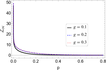
Figure 1: The variation of the logarithmic negativity between two Unruh-DeWitt detectors for a real conformal scalar field in the conformal vacuum with respect to the dimensionless energy parameter $p=2\omega/H$ and the field-detector coupling $g$. See main text for discussion.

III.2 The minimally coupled massless real scalar

Let us now consider a massless and minimally coupled ($m=0=\xi$) real scalar field. Note that this makes $\nu=3/2$ in 9, making it undefined. The two point function for such a scalar field needs to be obtained separately from its equation of motion, and the Wightman function is given by Allen:1985ux ,

$$iG^{+}(y)=\frac{H^{2}}{4\pi^{2}}\Bigg{(}\frac{1}{y}-\frac{\ln{y}}{2}+\frac{\ln{\big{(}a(\eta)a(\eta^{\prime})\big{)}}}{2}\Bigg{)}$$ (33)

Thus even though $y$ is de Sitter invariant, the above Wightman function is not, owing the logarithmic term of the scale factor. On substituting 33 in 20 and dividing by $\lim_{\tau_{+}\to\infty}\tau_{+}=(\tau_{A}+\tau^{\prime}_{B})/2$, we obtain the response function

$$P^{\prime}=\frac{dP}{d\tau+}=\frac{g^{2}H^{2}}{4\pi^{2}}\int_{-\infty}^{\infty}d(\Delta\tau)\;e^{-i\omega\Delta\tau}\Bigg{(}\frac{1}{y}-\frac{\ln{y}}{2}+\frac{\ln{\big{(}a(\eta)a(\eta^{\prime})\big{)}}}{2}\Bigg{)}$$ (34)

The above integral was first evaluated in Garbrecht:2004du , given by

$$P^{\prime}=\frac{pH}{4\pi}\frac{1+16/p^{2}}{e^{\pi p}-1}+\frac{H}{4\pi^{2}}\ln(a(t)a(t^{\prime}))\delta(p)$$ (35)

where $p=2\Delta E/H$ is dimensionless. We drop the $\delta$-function as earlier, owing to $p\neq 0$. Accordingly, similar to the case of the conformal scalar discussed in the previous section, 21 shows that $E^{\prime}=0$. The logarithmic negativity is formally the same as 32. Its variation with respect to parameter $p$ for different $g$ values is shown in 2.

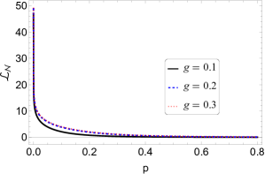
Figure 2: The variation of the logarithmic negativity for the minimally coupled massless real scalar with respect to the dimensionless energy gap $p$, as well as the field-detector coupling.

IV A complex scalar field coupled to Unruh-DeWitt detectors

Let us now come to the case of two Unruh-DeWitt detectors coupled to each other via a complex scalar field. Corresponding to 11, the interaction Hamiltonian is given by

$$H_{I}(t(\tau_{j}))=\sum_{j}g_{j}\mu_{j}(\tau_{j})\phi^{\dagger}(\vec{x}(\tau_{j}),t(\tau_{j}))\phi(\vec{x}(\tau_{j}),t(\tau_{j}))$$ (36)

where the index $j=A,B$ runs for both the detectors $A$ and $B$. We assume as earlier that the initial state of the scalar field is vacuum, as well as the detectors are in the ground state

$$|\text{in}\rangle=|0G_{A}G_{B}\rangle$$ (37)

where we have suppressed the tensor product symbol. The time evolution operator $U$ gives the ‘out’ state

$$|\text{out}\rangle=U|\text{in}\rangle=Te^{-i\int d\tau_{j}H_{I}(t(\tau_{j}))}|0G_{A}G_{B}\rangle$$ (38)

From the ‘out’ density operator,

$$\rho^{\text{out}}=|\text{out}\rangle\langle\text{out}|,$$ (39)

we compute the reduced density matrix corresponding to the two detectors as earlier by tracing out the field $\phi$ degrees of freedom, given by

$$\rho_{AB}=\left(\begin{array}[]{cccc}1-N_{AA}-N_{BB}&0&0&M\\ 0&N_{AA}&N_{AB}&0\\ 0&N_{AB}^{*}&N_{BB}&0\\ M^{*}&0&0&0\end{array}\right)$$ (40)

where the matrix elements explicitly read

$$M=-g^{2}\int d\tau_{A}\int d\tau^{\prime}_{B}\;e^{-i\omega(\tau_{A}+\tau^{\prime}_{B})}(iG_{F}(x_{A},x^{\prime}_{B}))^{2}$$ (41)

and

$$\begin{split}N_{IJ}=g^{2}\int d\tau_{I}\int d\tau^{\prime}_{J}\;e^{-i\omega(\tau_{I}-\tau^{\prime}_{J})}(-iG^{+}(x_{I},x^{\prime}_{J})))^{2}\end{split}$$ (42)

where $G^{+}(x_{J},x^{\prime}_{J})$ and $G_{F}(x_{J},x^{\prime}_{J})$ are the positive frequency Whitman propagator and the Feynman propagator, respectively. Note that 41 contains only the cross-detector coupling, whereas 42 also contains self coupling, both mediated via the scalar field. For identical detectors, 40 simplifies to

$$\rho_{AB}=\left(\begin{array}[]{cccc}1-2N&0&0&M\\ 0&N&N&0\\ 0&N&N&0\\ M^{*}&0&0&0\end{array}\right)$$ (43)

The above density matrix is formally similar to 22, although the elements are different, owing to 41 and 42, which contains the square of the propagator as opposed to the real scalar case. Defining once again measurement per unit proper time ($\tau_{+}$) as earlier, we obtain the logarithmic negativity for complex scalar field-detector coupling

$$\mathcal{L_{N}}=\log_{2}(4N^{\prime}(1+\sqrt{2})+1)$$ (44)

where compared to the case of the real scalar field, $N^{\prime}$ now contains the square of the Green function,

$$N^{\prime}=g^{2}\int_{-\infty}^{\infty}d(\Delta\tau)\;e^{-i\omega\Delta\tau}\;(iG^{+}(\Delta\tau))^{2}$$ (45)

IV.1 Conformal complex scalar in conformal vacuum

Let us first consider a conformal complex scalar field in the conformal vacuum. 45 in this case reads

$$N^{\prime}=\frac{g^{2}H^{3}}{128\pi^{4}}\int_{-\infty}^{\infty}du\,\frac{e^{-ipu}}{(\sinh u-i\epsilon)^{4}}=\frac{g^{2}p^{3}H^{3}}{384\pi^{3}}\frac{1}{e^{\pi p}-1}$$ (46)

where $p=2\Delta E/H$ as earlier. On substituting the above into 44, we obtain the logarithmic negativity for the two identical detectors coupled to a conformal complex scalar field in the conformal vacuum. Its variation with respect to the parameter $p$ for different values of the coupling $g$ is depicted in 3. Compared to the earlier cases of real scalar fields, 1, 2, we note a non-monotonic behaviour.

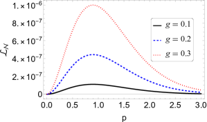
Figure 3: The variation of the logarithmic negativity for two identical detectors coupled to a conformal complex scalar field in a conformal vacuum with respect to the dimensionless energy gap $p$ and the coupling $g$. We note the qualitative difference compared to the monotonic behaviour of the real scalar field cases, 1, 2.

IV.2 The minimally coupled massless complex scalar

Let us now come to the case of a massless and minimally coupled scalar field. Substituting 33 into 45, we have

$$N^{\prime}=\frac{g^{2}H^{3}}{8\pi^{4}}\,\int_{-\infty}^{\infty}du\,e^{-ipu}\left[\frac{(y\ln y-2)^{2}}{4y^{2}}+\ln(a(t)a(t^{\prime}))\,\left(\frac{1}{y}-\frac{1}{2}\ln y\right)+\left(\frac{1}{2}\ln(a(t)a(t^{\prime}))\right)^{2}\right]\hskip 14.22636pt$$ (47)

We rewrite the above equation as (after ignoring a term proportional to $\delta(p)$),

$$N^{\prime}=\frac{H^{3}}{8\pi^{4}}\int_{-\infty}^{\infty}du\,e^{-ipu}\left[\frac{\left[2(\sinh u-i\epsilon)^{2}\ln(-4(\sinh u-i\epsilon)^{2})+1\right]^{2}}{16(\sinh u-i\epsilon)^{4}}-\frac{\ln(a(t)a(t^{\prime}))}{4(\sinh u-i\epsilon)^{2}}\right.$$

$$\left.-\left(\frac{1}{2}\ln(a(t)a(t^{\prime}))\right)\,\ln(-4(\sinh u-i\epsilon)^{2})\right]$$ (48)

The above integral was first evaluated in SKS , which we wish to outline below and in A, very briefly.

The first integral of 48 splits into three sub-integrals

$$\int_{-\infty}^{\infty}du\,e^{-ipu}\left[\frac{1}{16(\sinh u-i\epsilon)^{4}}+\frac{\ln\left(-4(\sinh u-i\epsilon\right)^{2})}{4(\sinh u-i\epsilon)^{2}}+\frac{\left(\ln\left(-4(\sinh u-i\epsilon)^{2}\right)\right)^{2}}{4}\right]$$ (49)

Note that the first integral in 49 is the same as that of the conformal complex scalar case 46. We now evaluate the second integral of 49. Expanding the logarithm in order to avoid the branch cuts, the second integral becomes

$$-\frac{1}{2}\sum_{n=1}^{\infty}\frac{1}{n}\int_{0}^{\infty}du\,\left(\frac{e^{-(ip+2n)u}}{\left(\sinh u-i\epsilon\right)^{2}}\,+\,{\rm c.c.}\right)\,+\,\frac{i}{2}\left(\partial_{p}+\frac{\pi}{2}\right)\int_{0}^{\infty}du\,\left(\frac{e^{-ipu}}{\left(\sinh u-i\epsilon\right)^{2}}\,-\,{\rm c.c.}\right)$$ (50)

where ‘c.c.’ stands for complex conjugation. The above integral shows divergences. We regularise them by renormalising the off-diagonal matrix elements of the detectors’ monopole operators in the energy eigenbasis, A (SKS ). The regularised expression reads

$$\int_{-\infty}^{\infty}du\,e^{-ipu}\,\frac{\ln\left(-4(\sinh u-i\epsilon\right)^{2})}{4(\sinh u-i\epsilon)^{2}}\Bigg{|}_{\rm Regularised}$$

$$= \frac{\pi}{2}\operatorname{csch}\frac{\pi p}{2}\coth\frac{\pi p}{2}\,\int_{0}^{\pi/2}\,dx\,\csc^{2}x\,\left[\cosh\left(\frac{\pi}{2}-x\right)p-\cosh\frac{\pi p}{2}+px\sinh\frac{\pi p}{2}\right]$$ (51)

$$-\operatorname{csch}\frac{\pi p}{2}\,\int_{0}^{\pi/2}\,dx\,\csc^{2}x\,\left[\left(\frac{\pi}{2}-x\right)\sinh\left(\frac{\pi}{2}-x\right)p-\left(\frac{\pi}{2}-x\right)\sinh\frac{\pi p}{2}+\frac{\pi px}{2}\cosh\frac{\pi p}{2}\right]$$

$$-\frac{\pi}{e^{\pi p}-1}\,\int_{0}^{\pi/2}\,dx\,\csc^{2}x\,\left[e^{px}-1-px\right]-\operatorname{csch}\frac{\pi p}{2}\,\int_{0}^{\pi/2}\,dx\,x\,\csc^{2}x\,\left[\sinh\left(\frac{\pi}{2}-x\right)p-\sinh\frac{\pi p}{2}\right]\hskip 28.45274pt$$

The third integral of 47 is given by

$$\int_{-\infty}^{\infty}du\;e^{-ipu}\frac{(\ln({-4(\sinh{u}-i\epsilon)^{2}}))^{2}}{4}=4\sum_{n=1}^{\infty}\frac{p^{2}-4n^{2}}{n(p^{2}+4n^{2})^{2}}-\sum_{n=1}^{\infty}\frac{2\pi p}{n(p^{2}+4n^{2})}+8\sum_{m,n=1}^{\infty}\,\frac{1}{n\,(p^{2}+4(m+n)^{2})}$$ (52)

Next, the second and third integrals of 48 can be evaluated in a likewise manner. Putting things together now, we obtain the regularised expression for the response function integral 48,

$$N^{\prime}_{\rm Regularised}=\frac{g^{2}p^{3}H^{3}}{384\pi^{3}}\,\frac{1}{e^{\pi p}-1}+\,\frac{pH^{3}}{16\pi^{3}}\,\frac{\ln(a(t)a(t^{\prime}))}{e^{\pi p}-1}\left(1+\frac{8}{p^{2}}\right)$$

$$+\frac{H^{3}}{2\pi^{4}}\left[\sum_{n=1}^{\infty}\frac{p^{2}-4n^{2}}{n(p^{2}+4n^{2})^{2}}-\sum_{n=1}^{\infty}\frac{\pi p}{2n(p^{2}+4n^{2})}+2\sum_{m,n=1}^{\infty}\,\frac{1}{n\,(p^{2}+4(m+n)^{2})}\right]$$

$$+\frac{H^{3}}{16\pi^{3}}\operatorname{csch}\frac{\pi p}{2}\coth\frac{\pi p}{2}\,\int_{0}^{\pi/2}\,dx\,\csc^{2}x\,\left[\cosh\left(\frac{\pi}{2}-x\right)p-\cosh\frac{\pi p}{2}+px\sinh\frac{\pi p}{2}\right]$$

$$-\frac{H^{3}}{8\pi^{4}}\operatorname{csch}\frac{\pi p}{2}\,\int_{0}^{\pi/2}\,dx\,\csc^{2}x\,\left[\left(\frac{\pi}{2}-x\right)\sinh\left(\frac{\pi}{2}-x\right)p-\left(\frac{\pi}{2}-x\right)\sinh\frac{\pi p}{2}+\frac{\pi px}{2}\cosh\frac{\pi p}{2}\right]$$

$$-\frac{H^{3}}{8\pi^{4}}\operatorname{csch}\frac{\pi p}{2}\,\int_{0}^{\pi/2}\,dx\,x\,\csc^{2}x\,\left[\sinh\left(\frac{\pi}{2}-x\right)p-\sinh\frac{\pi p}{2}\right]-\frac{H^{3}}{8\pi^{3}}\frac{\pi}{e^{\pi p}-1}\,\int_{0}^{\pi/2}\,dx\,\csc^{2}x\,\left[e^{px}-1-px\right]\hskip 34.14322pt$$ (53)

On substituting $N^{\prime}$ from 53 in 44, the logarithmic negativity can be computed and its variation with respect to parameter $p$ for different $g$ values can be seen in 4.

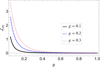
Figure 4: The variation of the logarithmic negativity for the minimally coupled massless complex scalar field with respect to the dimensionless energy gap $p$, for different values of the field-detector coupling $g$.

V Conclusion

Let us summarise our work now. In this paper we have computed the entanglement harvesting for two identical, two-level, comoving detectors in the cosmological de Sitter spacetime. The detectors are assumed to have coincident spatial position. We also have assumed that they are un-entangled initially. We have considered conformally invariant and massless minimally coupled scalar fields, and have considered both real and complex scalars. The entanglement generated between the detectors is computed in terms of the logarithmic negativity, depicted in 1, 2, 3, 4. We note that the first two and the fourth show monotonic behaviour for the log-negativity. Intuitively, we may explain this by noting that as the dimensionless energy difference between the levels of the detector, $p$, increases, the associated wavelength decreases, decreasing the correlation between the two detectors. 3 in this sense is counter-intuitive, for it shows a maximum for small $p$ values. We also note from 2 and 4 that there is more generation of log-negativity for complex field compared to the real for the massless minimally coupled case, for given values of the parameters.

Looking into the generation of decoherence between initially entangled detectors seems to be an interesting task in this context. Extension of the critical slowing down of a detector e.g. Kaplanek:2019vzj ; Burgess:2024eng to two initially unentangled or entangled ones seems also to be a very interesting task. We wish to come back to these issues in our future publications.

sectionAppendix #1

Appendix A Brief sketch of the computation of 48

Following SKS , we wish to provide below some detail for the evaluation of 48. For example for the evaluation of 50, we use

$$\int_{0}^{\infty}\,du\frac{e^{-ipu}}{\left(\sinh u-i\epsilon\right)^{2}}\,=-i\frac{\partial}{\partial\epsilon}\,\int_{0}^{\infty}\,du\frac{e^{-ipu}}{\left(\sinh u-i\epsilon\right)}$$ (54)

The above trick converts the second order pole to first order, so that we may assign a Cauchy principal value to the integral.

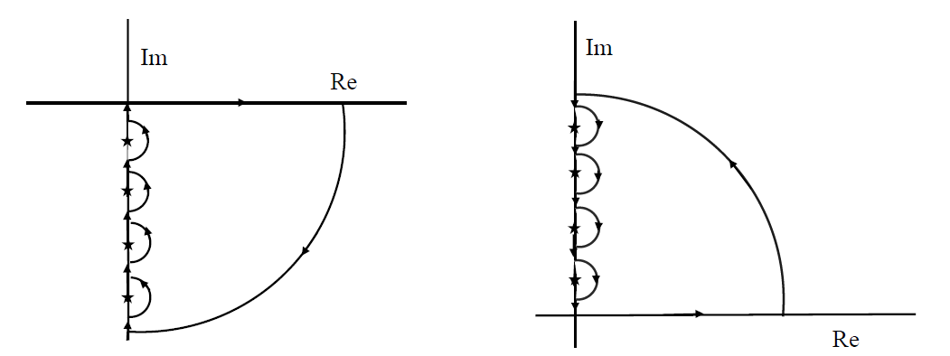
Figure 5: Contours required for the evaluation of integrals.

Accordingly, we utilise quarter-circular contours as shown in 5, with an infinite number of indentations around the poles

$$u_{n}=i(n\pi+(-1)^{n}\epsilon)\qquad n=0,\,\pm 1,\,\pm 2,\cdots$$

We have

$$\int_{0}^{\infty}\,du\;\frac{e^{-ipu}}{\left(\sinh u-i\epsilon\right)^{2}}\,=-\frac{\pi p}{e^{\pi p}-1}\,+\,i\,\int_{0}^{\infty}du\;\frac{e^{-pu}}{(\sin u+\epsilon)^{2}}\Bigg{|}_{\rm poles~{}excluded}$$ (55)

The above integral on the right hand side can be rewritten after a change of variable as,

$$\operatorname{csch}\frac{\pi p}{2}\,\int_{0}^{\pi/2}dx\;\csc^{2}x\,\cosh p\left(\frac{\pi}{2}-x\right)$$

By separating the divergence, we rewrite the above as

$$\coth\frac{\pi p}{2}\int_{0}^{\pi/2}dx\,\csc^{2}x-p\int_{0}^{\pi/2}dx\,x\,\csc^{2}x+\operatorname{csch}\frac{\pi p}{2}\int_{0}^{\pi/2}dx\csc^{2}x\left[\cosh\left(\frac{\pi}{2}-x\right)p-\cosh\frac{\pi p}{2}+px\sinh\frac{\pi p}{2}\right]$$

(56)

We also have

$$-\frac{1}{2}\sum_{n=1}^{\infty}\frac{1}{n}\int_{0}^{\infty}du\,\frac{e^{-(ip+2n)u}}{\left(\sinh u-i\epsilon\right)^{2}}+{\rm c.c.}=\frac{\pi p}{e^{p\pi}-1}\sum_{n=1}^{\infty}\frac{1}{n}+\frac{1}{\sinh\frac{\pi p}{2}}\sum_{n=1}^{\infty}\frac{1}{n}\int_{0}^{\pi/2}\,dx\,\csc^{2}x\sin 2nx\sinh\left(\frac{\pi}{2}-x\right)p$$

(57)

Using now the formula GR ,

$$\sum_{n=1}^{\infty}\frac{\sin 2nx}{n}=\frac{\pi-2x}{2}\qquad(0<x<\pi),$$ (58)

we rewrite 57 as

$$\frac{\pi p}{e^{p\pi}-1}\zeta(1)+\frac{\pi}{2}\int_{0}^{\pi/2}dx\,\csc^{2}x-\left(1+\frac{\pi p}{2}\coth\frac{\pi p}{2}\right)\,\int_{0}^{\pi/2}dx\,x\csc^{2}x$$

$$+\frac{\pi}{2\sinh\frac{\pi p}{2}}\int_{0}^{\pi/2}\,dx\,\csc^{2}x\,\left[\sinh\left(\frac{\pi}{2}-x\right)p-\sinh\frac{\pi p}{2}+px\cosh\frac{\pi p}{2}\right]$$

$$-\frac{1}{\sinh\frac{\pi p}{2}}\int_{0}^{\pi/2}\,dx\,x\,\csc^{2}x\,\left[\sinh\left(\frac{\pi}{2}-x\right)p-\sinh\frac{\pi p}{2}\right]$$ (59)

After inserting suitable regulators, we can extract the following divergent part

$$\int_{-\infty}^{\infty}du\,e^{-ipu}\,\frac{\ln\left(-4(\sinh u-i\epsilon\right)^{2})}{4(\sinh u-i\epsilon)^{2}}\Bigg{|}_{\rm div.}=\frac{\pi\coth\frac{\pi p}{2}}{e^{\pi p}-1}\frac{1}{\epsilon}+\frac{\pi p}{e^{\pi p}-1}\ln\frac{\epsilon}{\epsilon^{\prime}}$$ (60)

In order to regularise the above divergence, we modify the field-detector interaction by adding another monopole operator that does not couple to the field SKS , for any one of the detectors

$${\cal L}_{\rm int}=g\mu(t):\phi^{\dagger}(x(t))\phi(x(t)):+\mu^{\prime}(t)$$

The response function, 45, after this modification becomes (after ignoring a $\delta$-function as earlier),

$$N^{\prime}=\frac{2}{H}\int_{-\infty}^{\infty}du\,e^{-ipu}\,(iG^{+}(u))^{2}+\frac{2}{gH}\left(\frac{\langle E|\mu^{\prime}|G\rangle}{\langle E|\mu|G\rangle}+{\rm c.c.}\right)\int_{-\infty}^{\infty}du\,e^{-ipu}\,iG^{+}(u)$$ (61)

The first term on the right hand side gives the usual response function integral for a massless minimal complex scalar, 48, whereas the second term yields the response function for a real massless minimal scalar field. Here, $|G\rangle$ and $|E\rangle$ are the ground state and the excited state of the detector, respectively. In order for the above contribution to cancel the divergence of 60, we must set

$$\langle E|\mu^{\prime}|G\rangle=-\frac{gH^{3}}{8\pi^{2}p\left(1+16/p^{2}\right)}\left(\frac{\coth\frac{\pi p}{2}}{\epsilon}+p\ln\frac{\epsilon}{\epsilon^{\prime}}\right)\langle E|\mu|G\rangle$$ (62)

which implies an operator relationship,

$$\mu^{\prime}=-\frac{gH^{3}}{8\pi^{2}}\,\sum_{i,j,\,i\neq j}C_{ij}|i\rangle\langle i|\mu|j\rangle\langle j|$$ (63)

Next by denoting $|G\rangle$ and $|E\rangle$, respectively, say, $|i=0\rangle$ and $|i=1\rangle$, we obtain

$$C_{10}(p=2\omega/H)=\frac{1}{p(1+16/p^{2})}\left(\frac{\coth\frac{\pi p}{2}}{\epsilon}+p\ln\frac{\epsilon}{\epsilon^{\prime}}\right)$$ (64)

It is clear that, by construction, $\mu^{\prime}$ will cancel the divergence for any level transition of the detector. Note also that $C_{10}$ is even in $p$, i.e., $C_{01}=C_{10}$. On collecting all the finite pieces, the second integral of 49 is given by 51.

We next compute the third integral of 47. After some algebra, it can be cast into a form

$$-2\left(\partial_{p}^{2}+\pi\partial_{p}\right)\,\int_{0}^{\infty}du\,\cos pu-\sum_{n=1}^{\infty}\frac{1}{n}\,\left(4\partial_{p}+2\pi\right)\int_{0}^{\infty}du\,\sin pu\,e^{-2nu}$$

$$+2\sum_{m,n=1}^{\infty}\frac{1}{mn}\int_{0}^{\infty}du\,\cos pu\,e^{-2(m+n)u}$$ (65)

By introducing an infinitesimal positive imaginary part in $p$, we have

$$\int_{0}^{\infty}du\,\cos pu=0$$

Using the above result and also integrating by parts, 65 is evaluated as

$$4\sum_{n=1}^{\infty}\frac{p^{2}-4n^{2}}{n(p^{2}+4n^{2})^{2}}-\sum_{n=1}^{\infty}\frac{2\pi p}{n(p^{2}+4n^{2})}+8\sum_{m,n=1}^{\infty}\,\frac{1}{n\,(p^{2}+4(m+n)^{2})}$$ (66)

Putting everything together, the regularised expression of 53 follows.

References

- (1) A. Einstein, B. Podolsky and N. Rosen, Can Quantum-Mechanical Description of Physical Reality Be Considered Complete, Phys. Rev. 777 (1935)
- (2) S. Bell, On the Einstein-Podolsky-Rosen paradox, Physics1 195 (1964)
- (3) J. F. Clauser, M. A. Horne, A. Shimony and R. A. Holt, Proposed experiment to test local hidden-variable theories, Phys. Rev. Lett.23 880 (1969)
- (4) R. F. Werner, Quantum states with Einstein-Podolsky-Rosen correlations admitting a hidden-variable model, Phys. Rev. A 40, 4277 (1989)
- (5) M. A. Nielsen and I. L. Chuang (2010), Quantum Computation And Information Theory (Cambridge university press, UK)
- (6) W. Tittel, J. Brendel, H. Zbinden and N. Gisin, Violation of Bell inequalities by photons more than 10 km apart, Phys. Rev. Lett. 81, 3563-3566 (1998) [arXiv:quant-ph/9806043 [quant-ph]].
- (7) D. Salart, A. Baas, C. Branciard, N. Gisin and H. Zbinden, Testing spooky action at a distance , Nature 454, 861-864 (2008).
- (8) M. Hotta, Quantum measurement information as a key to energy extraction from local vacuums, Phys. Rev. D 78, 045006 (2008) [arXiv:0803.2272 [physics.gen-ph]].
- (9) M. Frey, K. Funo, and M. Hotta, Strong Local Passivity in Finite Quantum Systems , Phys.Rev.E 90, 012127 (2014).
- (10) I. Fuentes-Schuller and R. B. Mann, Alice falls into a black hole: Entanglement in non-inertial frames, Phys. Rev. Lett. 95, 120404 (2005) [arXiv:quant-ph/0410172 [quant-ph]].
- (11) B. Reznik, Entanglement from the vacuum, Found. Phys. 33, 167-176 (2003) [arXiv:quant-ph/0212044 [quant-ph]].
- (12) E. Martin-Martinez, A. R. H. Smith and D. R. Terno, Spacetime structure and vacuum entanglement, Phys. Rev. D 93, no.4, 044001 (2016) [arXiv:1507.02688 [quant-ph]].
- (13) I. Fuentes, R. B. Mann, E. Martin-Martinez and S. Moradi, Entanglement of Dirac fields in an expanding spacetime, Phys. Rev. D 82, 045030 (2010) [arXiv:1007.1569 [quant-ph]].
- (14) C. Anastopoulos, B. L. Hu and K. Savvidou, Quantum field theory based quantum information: Measurements and correlations, Annals Phys. 450, 169239 (2023) [arXiv:2208.03696 [quant-ph]].
- (15) H. Casini and M. Huerta, Lectures on entanglement in quantum field theory, PoS TASI2021, 002 (2023) [arXiv:2201.13310 [hep-th]].
- (16) John Preskill, Quantum information and physics: Some future directions, Journal of Modern 47, no. 2-3, 127-137, (2000).
- (17) Peres, Asher, Terno and R. Daniel, Quantum information and relativity theory, Rev. Mod. Phys., 76, no. 1, 93-123, (2004).
- (18) S. P. Jordan, K. S. M. Lee and J. Preskill, Quantum Computation of Scattering in Scalar Quantum Field Theories, Quant. Inf. Comput. 14, 1014-1080 (2014) [arXiv:1112.4833 [hep-th]].
- (19) S. B. Giddings, Black holes, quantum information, and unitary evolution, Phys. Rev. D 85, 124063 (2012 [arXiv:1201.1037 [hep-th]].
- (20) P. Calabrese and J. L. Cardy, Entanglement entropy and quantum field theory, J. Stat. Mech. 0406, P06002 (2004) [arXiv:hep-th/0405152 [hep-th]].
- (21) S. M. Wu, H. S. Zeng and T. Liu, Quantum correlation between a qubit and a relativistic boson in an expanding spacetime, Class. Quant. Grav. 39, no.13, 135016 (2022) [arXiv:2206.13733 [quant-ph]].
- (22) G. Menezes, Radiative processes of two entangled atoms outside a Schwarzschild black hole, Phys. Rev. D 94, no.10, 105008 (2016) [arXiv:1512.03636 [gr-qc]].
- (23) G. Menezes and N. F. Svaiter, Radiative processes of uniformly accelerated entangled atoms, Phys. Rev. A 93, no.5, 052117 (2016) [arXiv:1512.02886 [hep-th]].
- (24) S. Iso, N. Oshita, R. Tatsukawa, K. Yamamoto and S. Zhang, Quantum radiation produced by the entanglement of quantum fields, Phys. Rev. D 95, no.2, 023512 (2017) [arXiv:1610.08158 [hep-th]].
- (25) F. Lindel, A. Herter, V. Gebhart, J. Faist and S. Y. Buhmann, Entanglement Harvesting from Electromagnetic Quantum Fields, [arXiv:2311.04642 [quant-ph]].
- (26) C. Lima, E. Patterson, E. Tjoa and R. B. Mann, Unruh phenomena and thermalization for qudit detectors, Phys. Rev. D 108, no.10, 105020 (2023) [arXiv:2309.04598 [quant-ph]].
- (27) S. Elghaayda and M. Mansour, Entropy disorder and quantum correlations in two Unruh-deWitt detectors uniformly accelerating and interacting with a massless scalar field, Phys. Scripta 98, no.9, 095254 (2023)
- (28) D. Barman, S. Barman and B. R. Majhi, Entanglement harvesting between two inertial Unruh-DeWitt detectors from nonvacuum quantum fluctuations, Phys. Rev. D 106, no.4, 045005 (2022) [arXiv:2205.08505 [gr-qc]].
- (29) S. Kaushal, Schwinger effect and a uniformly accelerated observer, Eur. Phys. J. C 82, no.10, 872 (2022) [arXiv:2201.03906 [hep-th]].
- (30) W. G. Unruh, Notes on black-hole evaporation, Phys. Rev. D 14, 870 (1976)
- (31) F. Benatti and R. Floreanini, Entanglement generation in uniformly accelerating atoms: Reexamination of the Unruh effect, Phys. Rev. A 70, no.1, 012112 (2004) [arXiv:quant-ph/0403157 [quant-ph]].
- (32) G. Salton, R. B. Mann and N. C. Menicucci, Acceleration-assisted entanglement harvesting and rangefinding, New J. Phys. 17, no.3, 035001 (2015) [arXiv:1408.1395 [quant-ph]].
- (33) J. I. Koga, G. Kimura and K. Maeda, Quantum teleportation in vacuum using only Unruh-DeWitt detectors, Phys. Rev. A 97, no.6, 062338 (2018) [arXiv:1804.01183 [gr-qc]].
- (34) J. I. Koga, K. Maeda and G. Kimura, Entanglement extracted from vacuum into accelerated Unruh-DeWitt detectors and energy conservation, Phys. Rev. D 100, no.6, 065013 (2019) [arXiv:1906.02843 [quant-ph]].
- (35) J. Zhang and H. Yu, Entanglement harvesting for Unruh-DeWitt detectors in circular motion, Phys. Rev. D 102, no.6, 065013 (2020) [arXiv:2008.07980 [quant-ph]].
- (36) L. J. Henderson, R. A. Hennigar, R. B. Mann, A. R. H. Smith and J. Zhang, Harvesting Entanglement from the Black Hole Vacuum, Class. Quant. Grav. 35, no.21, 21LT02 (2018) [arXiv:1712.10018 [quant-ph]].
- (37) D. Wu, S. C. Tang and Y. Shi, Birth and death of entanglement between two accelerating Unruh-DeWitt detectors coupled with a scalar field, JHEP 12, 037 (2023)[arXiv:2304.12126 [gr-qc]].
- (38) E. Martin-Martinez and N. C. Menicucci, Cosmological quantum entanglement, Class. Quant. Grav. 29, 224003 (2012) [arXiv:1204.4918 [gr-qc]].
- (39) E. Tjoa and R. B. Mann, Unruh-DeWitt detector in dimensionally-reduced static spherically symmetric spacetimes, JHEP 03, 014 (2022) [arXiv:2202.04084 [gr-qc]].
- (40) D. Bhattacharya, K. Gallock-Yoshimura, L. J. Henderson and R. B. Mann, Extraction of entanglement from quantum fields with entangled particle detectors, Phys. Rev. D 107, no.10, 105008 (2023) [arXiv:2212.12803 [quant-ph]].
- (41) A. Dhanuka and K. Lochan, Unruh DeWitt probe of late time revival of quantum correlations in Friedmann spacetimes, Phys. Rev. D 106, no.12, 125006 (2022) [arXiv:2210.11186 [gr-qc]].
- (42) H. Maeso-García, J. Polo-Gómez and E. Martín-Martínez, How measuring a quantum field affects entanglement harvesting, Phys. Rev. D 107, no.4, 045011 (2023) [arXiv:2210.05692 [quant-ph]].
- (43) E. Martin-Martinez and B. C. Sanders, Precise space–time positioning for entanglement harvesting, New J. Phys. 18, 043031 (2016) [arXiv:1508.01209 [quant-ph]].
- (44) D. Mendez-Avalos, L. J. Henderson, K. Gallock-Yoshimura and R. B. Mann, Entanglement harvesting of three Unruh-DeWitt detectors, Gen. Rel. Grav. 54, no.8, 87 (2022)[arXiv:2206.11902 [quant-ph]].
- (45) T. R. Perche, B. Ragula and E. Martín-Martínez, Harvesting entanglement from the gravitational vacuum, Phys. Rev. D 108, no.8, 085025 (2023) [arXiv:2210.14921 [quant-ph]].
- (46) E. G. Brown, Thermal amplification of field-correlation harvesting, Phys. Rev. A 88, no.6, 062336 (2013) [arXiv:1309.1425 [quant-ph]].
- (47) S. Barman, D. Barman and B. R. Majhi, Entanglement harvesting from conformal vacuums between two Unruh-DeWitt detectors moving along null paths, JHEP 09, 106 (2022) [arXiv:2112.01308 [gr-qc]].
- (48) L. J. Henderson, S. Y. Ding and R. B. Mann, Entanglement harvesting with a twist, AVS Quantum Sci. 4, no.1, 014402 (2022) [arXiv:2201.11130 [quant-ph]].
- (49) T. Prokopec, Gravitational wave signals in an Unruh–DeWitt detector, Class. Quant. Grav. 40, no.3, 035007 (2023) [arXiv:2206.10136 [gr-qc]].
- (50) Q. Xu, S. A. Ahmad and A. R. H. Smith, Gravitational waves affect vacuum entanglement, Phys. Rev. D 102, no.6, 065019 (2020) [arXiv:2006.11301 [quant-ph]].
- (51) M. P. G. Robbins, L. J. Henderson and R. B. Mann, Entanglement amplification from rotating black holes, Class. Quant. Grav. 39, no.2, 02LT01 (2022) [arXiv:2010.14517 [hep-th]].
- (52) W. Cong, C. Qian, M. R. R. Good and R. B. Mann, Effects of Horizons on Entanglement Harvesting, JHEP 10, 067 (2020) [arXiv:2006.01720 [gr-qc]].
- (53) K. Gallock-Yoshimura, E. Tjoa and R. B. Mann, Harvesting entanglement with detectors freely falling into a black hole, Phys. Rev. D 104, no.2, 025001 (2021) [arXiv:2102.09573 [quant-ph]].
- (54) M. Cliche and A. Kempf, Vacuum entanglement enhancement by a weak gravitational field, Phys. Rev. D 83, 045019 (2011) [arXiv:1008.4926 [quant-ph]].
- (55) A. Pozas-Kerstjens and E. Martin-Martinez, Harvesting correlations from the quantum vacuum, Phys. Rev. D 92, no.6, 064042 (2015) [arXiv:1506.03081 [quant-ph]].
- (56) P. Chowdhury and B. R. Majhi, Fate of entanglement between two Unruh-DeWitt detectors due to their motion and background temperature, JHEP 05, 025 (2022) [arXiv:2110.11260 [hep-th]].
- (57) D. Barman, A. Choudhury, B. Kad and B. R. Majhi, Spontaneous entanglement leakage of two static entangled Unruh-DeWitt detectors, Phys. Rev. D 107, no.4, 045001 (2023) [arXiv:2211.00383 [quant-ph]].
- (58) D. Makarov, Quantum entanglement of a harmonic oscillator with an electromagnetic field, Sci. Rep. 8, no.1, 8204 (2018)
- (59) E. G. Brown, E. Martin-Martinez, N. C. Menicucci and R. B. Mann, Detectors for probing relativistic quantum physics beyond perturbation theory, Phys. Rev. D 87, 084062 (2013) [arXiv:1212.1973 [quant-ph]].
- (60) D. Boyanovsky, Imprint of entanglement entropy in the power spectrum of inflationary fluctuations, Phys. Rev. D 98, no.2, 023515 (2018) [arXiv:1804.07967[astro-ph.CO]]
- (61) D. Rauch, J. Handsteiner, A. Hochrainer, J. Gallicchio, A. S. Friedman, C. Leung, B. Liu, L. Bulla, S. Ecker and F. Steinlechner, et al. Cosmic Bell Test Using Random Measurement Settings from High-Redshift Quasars, Phys. Rev. Lett. 121, no.8, 080403 (2018) [arXiv:1808.05966[quant-ph]].
- (62) M. J. P. Morse, Statistical Bounds on CMB Bell Violation, [arXiv:2003.13562 [astro-ph.CO]]
- (63) S. Bhattacharya, S. Chakrabortty and S. Goyal, Dirac fermion, cosmological event horizons and quantum entanglement, Phys. Rev. D101, no.8, 085016 (2020) [arXiv:1912.12272 [hep-th]].
- (64) S. Bhattacharya, H. Gaur and N. Joshi, Some measures for fermionic entanglement in the cosmological de Sitter spacetime, Phys. Rev. D102, no.4, 045017 (2020) [arXiv:2006.14212 [hep-th]].
- (65) M. S. Ali, S. Bhattacharya, S. Chakrabortty and S. Kaushal, Fermionic Bell violation in the presence of background electromagnetic fields in the cosmological de Sitter spacetime, Phys. Rev. D104, no.12, 125012 (2021) [arXiv:2102.11745 [hep-th]].
- (66) J. Foo, S. Onoe, R. B. Mann and M. Zych, Thermality, causality, and the quantum-controlled Unruh–deWitt detector, Phys. Rev. Res. 3, no.4, 043056 (2021) [arXiv:2005.03914 [quant-ph]].
- (67) G. L. Ver Steeg and N. C. Menicucci, Entangling power of an expanding universe, Phys. Rev. D 79, 044027 (2009) [arXiv:0711.3066 [quant-ph]].
- (68) S. Brahma, J. Calderón-Figueroa, M. Hassan and X. Mi, Momentum-space entanglement entropy in de Sitter spacetime, Phys. Rev. D 108, no.4, 043522 (2023) [arXiv:2302.13894 [hep-th]]
- (69) S. Brahma and A. N. Seenivasan, Probing the curvature of the cosmos from quantum entanglement due to gravity, [arXiv:2311.05483 [gr-qc]].
- (70) A. Bhattacharyya, S. Brahma, S. S. Haque, J. S. Lund and A. Paul, The Early Universe as an Open Quantum System: Complexity and Decoherence, [arXiv:2401.12134 [hep-th]].
- (71) N. D. Birrell and P. C. W. Davies, Quantum Fields in Curved Space, Cambridge Univ. Press (1982).
- (72) B. Allen, Vacuum States in de Sitter Space, Phys. Rev. D 32, 3136 (1985).
- (73) J. Louko and V. Toussaint, Unruh-DeWitt detector’s response to fermions in flat spacetimes, Phys. Rev. D 94, no. 6, 064027 (2016) [arXiv:1608.01002 [gr-qc]].
- (74) M. S. Ali, S. Bhattacharya and K. Lochan, Unruh-DeWitt detector responses for complex scalar fields in de Sitter spacetime, JHEP 03, 220 (2021) [arXiv:2003.11046 [hep-th]].
- (75) S. Y. Lin, Unruh-DeWitt-type monopole detector in (3+1)-dimensional space-time, Phys. Rev. D, 68, 104019, (2003).
- (76) D. E. Bruschi, A. R. Lee and I. Fuentes, Time evolution techniques for detectors in relativistic quantum information, J. Phys. A 46, 165303 (2013) [arXiv:1212.2110 [quant-ph]].
- (77) L. Sriramkumar and T. Padmanabhan, Response of finite time particle detectors in noninertial frames and curved space-time, Class. Quant. Grav. 13, 2061-2079 (1996) [arXiv:gr-qc/9408037 [gr-qc]].
- (78) G. Vidal and R. F. Werner, Computable measure of entanglement, Phys. Rev. A 65, 032314 (2002) [arXiv:quant-ph/0102117].
- (79) M. B. Plenio, Logarithmic negativity: a full entanglement monotone that is not convex, Phys. Rev. Lett. 95, 090503 (2005)
- (80) P. Calabrese, J. Cardy and E. Tonni, Entanglement negativity in extended systems: A field theoretical approach J. Stat. Mech. 1302, P02008 (2013) [arXiv:1210.5359 [cond-mat.stat-mech]].
- (81) R. Bousso, A. Maloney and A. Strominger, Conformal vacua and entropy in de Sitter space, Phys. Rev. D 65, 104039 (2002) [arXiv:hep-th/0112218 [hep-th]].
- (82) B. Garbrecht and T. Prokopec, Unruh response functions for scalar fields in de Sitter space, Class. Quant. Grav. 21, 4993-5004 (2004) [arXiv:gr-qc/0404058 [gr-qc]].
- (83) G. Kaplanek and C. P. Burgess, Hot Cosmic Qubits: Late-Time de Sitter Evolution and Critical Slowing Down, JHEP 02, 053 (2020) [arXiv:1912.12955 [hep-th]].
- (84) C. P. Burgess, T. Colas, R. Holman, G. Kaplanek and V. Vennin, Cosmic Purity Lost: Perturbative and Resummed Late-Time Inflationary Decoherence, [arXiv:2403.12240 [gr-qc]].
- (85) I. S. Gradshteyn and I. M. Ryzhik, Table of integrals, series, and products, Academic Press, NY (1965).