Study of structure of deuteron from analysis of bremsstrahlung emission in proton-deuteron scattering in cluster models

Abstract

Purpose: In this paper we investigated emission of bremsstrahlung photons in the scattering of protons off deuterons within the microscopic cluster models in a wide region of the beam energy from low energies up to 1.5 GeV. Methods: Three-cluster model of bremsstrahlung is constructed for such a reaction. Formalism of the model includes form factor of deuteron which characterizes dependence of bremsstrahlung cross sections on structure of deuteron. This gives possibility to investigate the structure of nuclei from analysis of bremsstrahlung cross sections. Results: We studied dependence of the bremsstrahlung cross section on the structure of deuteron. We use three different shapes of the deuteron wave functions. Besides, we also calculate the cross section by neglecting internal structure of deuteron. Analysis of dependence of the cross section on such a parameter shows the following. (1) At beam energies 145 and 195 MeV used in experiments bremsstrahlung cross section is not sensitive visibly on variations of the shape of the deuteron wave functions. (2) Stable difference between cross sections calculated with and without internal structure of deuteron is observed at higher energy of beam (larger 500 MeV). (3) The spectrum is increased as we pass from structureless deuteron (the oscillator length $b$=0) to the deuteron discribed by the shell-model wave function (the realistic oscillator length) inside the full energy region of the emitted photons. Conclusion: Our cluster model is a suitable tool to study the structure of deuteron with high enough precision from bremsstrahlung analysis. We propose new experiments for such an investigation.

I Introduction

The bremsstrahlung emission of photons accompanying nuclear reactions is an important topic of nuclear physics and has been attracted a significant interest of many researchers for a long time (see reviews Amusia.1988.PhysRep ; Pluiko.1987.PEPAN ; Kamanin.1989.PEPAN ; Bertulani.1988.PhysRep ). This is explained by that the spectra of bremsstrahlung photons are calculated on the basis of nuclear models which include mechanisms of reactions, interactions between nuclei, dynamics, and many other physical issues. A lot of aspects of nuclear processes, such as dynamics of nucleons in the nuclear scattering, interactions between nucleons, mechanisms of reactions, quantum effects, deformations of nuclei, properties of hypernuclei in reactions, etc. can be included to the model describing the bremsstrahlung emission (for example, see Refs. Maydanyuk.2003.PTP ; Maydanyuk.2006.EPJA for general properties of $\alpha$ decay from bremsstrahlung analysis, Ref. Maydanyuk.2009.NPA for extraction of information about deformation of nuclei in the $\alpha$ decay from experimental bremsstrahlung data, Ref. Maydanyuk.2011.JPG for bremsstrahlung in the nuclear radioactivity with emission of protons, Ref. Maydanyuk.2010.PRC for bremsstrahlung in the spontaneous fission of [252]Cf, Ref. Maydanyuk.2011.JPCS for bremsstrahlung in the ternary fission of [252]Cf, Ref. Maydanyuk_Zhang_Zou.2018.PRC for bremsstrahlung in the pion-nucleus scattering from our research, there are many investigations of other researchers). Note perspectives on studying electromagnetic observables of light nuclei based on chiral effective field theory Pastore.2008.PRC . The measurements of photons with analysis provide important information on these phenomena.

Analysis of bremsstrahlung photons accompanying nuclear reactions gives possibility to extract additional information on structure of nuclei. Study of the structure of nuclei on the basis of bremsstrahlung analysis is one of the most ambitious aims in nuclear physics. Analyzing formalism of models, option to investigate structure of nuclei exists, in principle, and understandable. Study of structure of nuclei is one of the most promising research directions, taking into account that photons can be measured in experiments. However, during long period of investigations of bremsstrahlung photons in nuclear physics, systematic study of structure of nuclei has not been realized yet. One can explain that by difficulty in development of mathematical formalism of models, importance to reach stability of numerical calculations that is possible at high precision. Moreover, it turns out that not all available experimental bremsstrahlung data are well sensitive to structure of nuclei. In this regards, one can remind investigations of bremsstrahlung emission in reactions with light nuclei within microscopic two-cluster models 1985NuPhA.443..302B ; 1990PhRvC..41.1401L ; 1990PhRvC..42.1895L ; 1991NuPhA.529..467B ; 1991PhRvC..44.1695L ; 1992NuPhA.550..250B ; Liu.1992.FBS ; 1993nuco.conf..423K ; Dohet-Eraly.2011.JPCS ; Dohet-Eraly.2011.PRC ; Dohet-Eraly.2013.PRC ; 2013JPhCS.436a2030D ; Dohet-Eraly.2013.PhD ; 2014PhRvC..89b4617D ; 2014PhRvC..90c4611D .

Summarizing all issues mentioned above, we see perspective problem on realization of such an idea, that is a main aim of this paper. We would like to understand, which parameters of nuclear structure are more effective to realize such an investigation. Of course, the best way is to construct this model on the fully quantum basis, with inclusion of realistic nuclear interactions which were well tested experimentally. A promising way is cluster formalism for description of structure of nuclei and nuclear process. So, as a basis of this research we will develop the fully cluster model in combination of bremsstrahlung formalism. The most effective process for such study is proton-deuteron scattering. We focus on construction of such a unified cluster formalism, analysis of available experimental information about bremsstrahlung for proton-deuteron scattering. This paper is continuation of our previous research Maydanyuk_Vasilevsky.2023.PRC , where we developed cluster model in the folding approximation in study of bremsstrahlung emission in the scattering of nuclei with the small number of nucleons and we did not analyze possibility to extract information about structure of nuclei from bremsstrahlung cross sections.

The paper is organized in the following way. In Sec. II cluster models of emission of the bremsstrahlung photons in the proton-deuteron scattering is formulated. Here, we give an explicit form of the operator of the bremsstrahlung emission, define wave functions of $p+d$ system, calculate matrix elements of bremsstrahlung emission, define form factors of deuteron (characterizing its structure), apply the multiple expansion approach for calculation of matrix elements. In Sec. IV matrix elements of bremsstrahlung emission in folding approximation are reviewed (following to formalism in Ref. Maydanyuk_Vasilevsky.2023.PRC ). In Sec. V cross section of the bremsstrahlung emission of photons is determined and resulting formulas are summarized. In Sec. VI emission of the bremsstrahlung photons for the proton-deuteron scattering is studied on the basis of the model above. We analyze role of the deuteron wave function and its form factor in calculations of the cross section at different energies of relative motions between the scattered proton and deuteron. We also describe the experimental bremsstrahlung data for the proton-deuteron scattering on the basis of the model. Conclusions and perspectives are summarized in Sec. VII. Operator of bremsstrahlung emission in three-cluster model is calculated in App. A. Useful details of calculation of integrals are presented in App. B. Form factor of deuteron in three-cluster approach is derived in App. C.

II Matrix elements of bremsstrahlung emission in three-cluster model

II.1 Operator of bremsstrahlung emission in three-cluster model

Consider the translationally invariant interaction of photon with three-nucleon system

$$\widehat{H}_{e}\left(\mathbf{k}_{\gamma},\mathbf{\varepsilon}^{(\alpha)}\right)=\frac{1}{2}\frac{e\hbar}{m_{N}c}\sum_{i=1}^{A=3}\frac{1}{2}\left(1+\widehat{\tau}_{iz}\right)\left[\widehat{\mathbf{\pi}}_{i}^{\ast}\mathbf{A}^{\ast}\left(i\right)+\mathbf{A}^{\ast}\left(i\right)\widehat{\mathbf{\pi}}_{i}^{\ast}\right]$$ (1)

where

$$\begin{array}[]{lllllll}\vspace{1.0mm}\mathbf{A}^{\ast}\left(i\right)=\mathbf{\varepsilon}^{(\alpha)}\exp\left\{-i\left(\mathbf{k}_{\gamma}\mathbf{\rho}_{i}\right)\right\},&\widehat{\mathbf{\pi}}_{i}^{\ast}=i\nabla_{\mathbf{\rho}_{i}},&\mathbf{\rho}_{i}=\mathbf{r}_{i}-\mathbf{R}_{\rm cm},\\ \mathbf{R}_{cm}=\displaystyle\frac{1}{A}\displaystyle\sum_{i=1}^{A}\mathbf{r}_{i},&\widehat{\mathbf{\pi}}_{i}=\widehat{\mathbf{p}}_{i}-\widehat{\mathbf{P}}_{cm},&\widehat{\mathbf{P}}_{cm}=\displaystyle\frac{1}{A}\displaystyle\sum_{i=1}^{A}\widehat{\mathbf{p}}_{i}.\end{array}$$ (2)

Here, $\mbox{\boldmath$\varepsilon$}^{(\alpha)}$ are unit vectors of linear polarization of the photon emitted ($\mbox{\boldmath$\varepsilon$}^{(\alpha),*}=\mbox{\boldmath$\varepsilon$}^{(\alpha)}$), $\mathbf{k}_{\gamma}$ is wave vector of the photon and $w_{\gamma}=k_{\gamma}c=\bigl{|}\mathbf{k}_{\gamma}\bigr{|}c$. Vectors $\mbox{\boldmath$\varepsilon$}^{(\alpha)}$ are perpendicular to $\mathbf{k}_{\gamma}$ in Coulomb gauge. We have two independent polarizations $\mbox{\boldmath$\varepsilon$}^{(1)}$ and $\mbox{\boldmath$\varepsilon$}^{(2)}$ for the photon with impulse $\mathbf{k}_{\gamma}$ ($\alpha=1,2$). Also we have properties:

$$\begin{array}[]{lclc}\Bigl{[}\mathbf{k}_{\gamma}\times\mbox{\boldmath$\varepsilon$}^{(1)}\Bigr{]}=k_{\gamma}\,\mbox{\boldmath$\varepsilon$}^{(2)},&\Bigl{[}\mathbf{k}_{\gamma}\times\mbox{\boldmath$\varepsilon$}^{(2)}\Bigr{]}=-\,k_{\gamma}\,\mbox{\boldmath$\varepsilon$}^{(1)},&\Bigl{[}\mathbf{k}_{\gamma}\times\mbox{\boldmath$\varepsilon$}^{(3)}\Bigr{]}=0,&\displaystyle\sum\limits_{\alpha=1,2,3}\Bigl{[}\mathbf{k}_{\gamma}\times\mbox{\boldmath$\varepsilon$}^{(\alpha)}\Bigr{]}=k_{\gamma}\,(\mbox{\boldmath$\varepsilon$}^{(2)}-\mbox{\boldmath$\varepsilon$}^{(1)}).\end{array}$$ (3)

Let us introduce new variables, namely Jacobi vectors $\mathbf{r}$ and $\mathbf{q}$

$$\begin{array}[]{lllll}\mathbf{r}=\displaystyle\frac{1}{\sqrt{2}}\left(\mathbf{\rho}_{1}-\mathbf{\rho}_{2}\right)=\displaystyle\frac{1}{\sqrt{2}}\left(\mathbf{r}_{1}-\mathbf{r}_{2}\right),\quad\mathbf{q}=\sqrt{\displaystyle\frac{2}{3}}\left(\mathbf{\rho}_{3}-\frac{\mathbf{\rho}_{1}+\mathbf{\rho}_{2}}{2}\right)=\sqrt{\frac{2}{3}}\left(\mathbf{r}_{3}-\displaystyle\frac{\mathbf{r}_{1}+\mathbf{r}_{2}}{2}\right),\\ \mathbf{q}_{A}=\sqrt{\displaystyle\frac{1}{3}}\left(\mathbf{r}_{1}+\mathbf{r}_{2}+\mathbf{r}_{3}\right)=\sqrt{3}\mathbf{R}_{cm}.\end{array}$$

Inverse relations are

$$\begin{array}[]{lllll}\mathbf{r}_{1}=\displaystyle\frac{1}{\sqrt{2}}\mathbf{r}-\displaystyle\frac{1}{\sqrt{6}}\mathbf{q}+\displaystyle\frac{1}{\sqrt{3}}\mathbf{q}_{A},&\mathbf{r}_{2}=-\displaystyle\frac{1}{\sqrt{2}}\mathbf{r}-\displaystyle\frac{1}{\sqrt{6}}\mathbf{q}+\displaystyle\frac{1}{\sqrt{3}}\mathbf{q}_{A},&\mathbf{r}_{3}=\displaystyle\sqrt{\frac{2}{3}}\mathbf{q}+\displaystyle\frac{1}{\sqrt{3}}\mathbf{q}_{A}.\end{array}$$ (4)

Similar relations can be written for momenta

$$\mathbf{\pi}_{\mathbf{r}} =\frac{1}{\sqrt{2}}\left(\mathbf{\pi}_{1}-\mathbf{\pi}_{2}\right),$$

$$\mathbf{\pi}_{\mathbf{q}} =\sqrt{\frac{2}{3}}\left(\mathbf{\pi}_{3}-\frac{\mathbf{\pi}_{1}+\mathbf{\pi}_{2}}{2}\right),$$

$$\mathbf{\pi}_{A} =\sqrt{\frac{1}{3}}\left(\mathbf{\pi}_{1}+\mathbf{\pi}_{2}+\mathbf{\pi}_{3}\right).$$

Inverse relations

$$\mathbf{\pi}_{1} =\frac{1}{\sqrt{2}}\mathbf{\pi}_{\mathbf{r}}\mathbf{-}\frac{1}{\sqrt{6}}\mathbf{\pi}_{\mathbf{q}}\mathbf{+}\frac{1}{\sqrt{3}}\mathbf{\pi}_{A},$$

$$\mathbf{\pi}_{2} =-\frac{1}{\sqrt{2}}\mathbf{\pi}_{\mathbf{r}}\mathbf{-}\frac{1}{\sqrt{6}}\mathbf{\pi}_{\mathbf{q}}\mathbf{+}\frac{1}{\sqrt{3}}\mathbf{\pi}_{A},$$

$$\mathbf{\pi}_{3} =\sqrt{\frac{2}{3}}\mathbf{\pi}_{\mathbf{q}}\mathbf{+}\frac{1}{\sqrt{3}}\mathbf{\pi}_{A}.$$

Now we fix position of nucleons. We assume that vector $\mathbf{r}$ measures the distance between proton and neutron which form a deuteron. We also assume that $\mathbf{r}_{1}$ is a coordinate of the first proton and $\mathbf{r}_{2}$ is a coordinate of a neutron. Vector $\mathbf{r}_{3}$ determines the location of the second proton. With such definitions, the operator $\widehat{H}_{e}\left(\mathbf{k}_{\gamma},\mathbf{\varepsilon}^{(\alpha)}\right)$ is [see App. A for details, also we take into account that $\left(\mathbf{\varepsilon}^{(\alpha)},\mathbf{k}_{\gamma}\right)=0$]

$$\begin{array}[]{lllll}\vspace{1.5mm}\widehat{H}_{e}\left(\mathbf{k}_{\gamma},\mathbf{\varepsilon}^{(\alpha)}\right)&=&\displaystyle\frac{1}{2}\displaystyle\frac{e\hbar}{m_{N}c}\biggl{\{}\displaystyle\frac{2}{\sqrt{2}}\exp\left\{-i\displaystyle\frac{1}{\sqrt{2}}\left(\mathbf{k}_{\gamma}\mathbf{r}\right)\right\}\left(\mathbf{\varepsilon}^{(\alpha)},\mathbf{\pi}_{\mathbf{r}}^{\ast}\right)\exp\left\{i\frac{1}{\sqrt{6}}\left(\mathbf{k}_{\gamma}\mathbf{q}\right)\right\}\,-\\ &-&\sqrt{\displaystyle\frac{2}{3}}\exp\left\{-i\displaystyle\frac{1}{\sqrt{2}}\left(\mathbf{k}_{\gamma}\mathbf{r}\right)\right\}\exp\left\{i\displaystyle\frac{1}{\sqrt{6}}\left(\mathbf{k}_{\gamma}\mathbf{q}\right)\right\}\left(\mathbf{\varepsilon}^{(\alpha)},\mathbf{\pi}_{\mathbf{q}}^{\ast}\right)+2\sqrt{\displaystyle\frac{2}{3}}\exp\{-i\sqrt{\displaystyle\frac{2}{3}}\left(\mathbf{k}_{\gamma}\mathbf{q}\right)\biggr{\}}\left(\mathbf{\varepsilon}^{(\alpha)},\mathbf{\pi}_{\mathbf{q}}^{\ast}\right)\biggr{\}}.\end{array}$$ (5)

This is the universal and model-independent form of the operator of bremsstrahlung emission for a system comprising from two protons and one neutron. To calculated cross section of bremsstrahlung emission in the process of a proton scattering from a deuteron, we need to formulate model which provides a realistic description of the $p+d$ scattering in economical way, i.e. with minimum of computations but with a reliable output. As the output, we need to determine wave functions of the $p+d$ scattering at selected energies of initial and final states of bremsstrahlung emission. For this aim, we select the resonating group method (RGM), which is the most rigorous and self-consistent realization of a cluster model. Actually, we will use three different variants of the RGM: two- and three-cluster variants and so-called the folding approximation. These three variants of the RGM are explained in detail in next Section.

III Two and three-cluster models of $p+d$ system

Three-nucleon system ³He and its decay channel $p+d$ will be studied in the framework of two- and three-cluster models. In a two-cluster model, wave function of the system is

$$\Psi=\widehat{\mathcal{A}}\left\{\phi^{(S)}\left(d,\mathbf{r}\right)\phi\left(p\right)\psi_{E}\left(\mathbf{q}\right)\right\},$$ (6)

where $\phi^{(S)}\left(d,\mathbf{r}\right)$ is the deuteron wave function from the oscillator shell-model, $\phi\left(p\right)$ is a wave function of proton represented by its spin and isospin parts, and $\psi_{E}\left(\mathbf{q}\right)$ is a wave function of relative motion of proton and deuteron. The antisymmetrization operator $\widehat{\mathcal{A}}$ makes wave functions of the $p+d$ system fully antisymmetric. Three-cluster model suggests the following form for three-nucleon system

$$\Psi=\widehat{\mathcal{A}}\left\{\phi\left(n\right)\phi\left(p_{1}\right)\phi\left(p_{2}\right)f\left(\mathbf{r,q}\right)\right\},$$ (7)

Wave function $\phi\left(p_{2}\right)f\left(\mathbf{r,q}\right)$ of relative motion of nucleons has to be determined by solving the Schrödinger equation or the Faddeev equations.

By assuming that the shape of a deuteron does not change when proton is approaching, then three-particle wave function can be represented as

$$\Psi=\widehat{\mathcal{A}}\left\{\phi\left(d,\mathbf{r}\right)\phi\left(p\right)\psi_{E}\left(\mathbf{q}\right)\right\},$$ (8)

where $\phi\left(d,\mathbf{r}\right)$ is a wave function of the bound state of deuteron. The wave function $\phi\left(d,\mathbf{r}\right)$ is a solution of two-body Schrödinger equation with selected nucleon-nucleon potential.

Note that in both models, in two-cluster and three-cluster, the wave function of deuteron is assumed to be antisymmetric, than the antisymmetrization operator $\widehat{\mathcal{A}}$ in Eqs. (6) and  (8) consists of the unit operator and two permutation operators. As the results, the antisymmetrization operator $\widehat{\mathcal{A}}$ creates in Eqs. (6) and  (8) three terms which are similar to the terms in curly brackets.

If one ignores the full antisymmetrization in Eqs. (6) and (8) by omitting the operator $\widehat{\mathcal{A}}$, one obtains a simple version of the two- and three-cluster models which is called a folding approximation or folding model. In order to avoid bulky expressions, we will use this approximation to present matrix elements of the $\widehat{H}_{e}\left(\mathbf{k}_{\gamma},\mathbf{\varepsilon}_{\mu}\right)$ between the initial and final states of the $p+d$ system.

To construct wave functions of the system $p+d$ in different approximations (models), we need to solve the appropriate Schrödinger equations. For this aim we employ the algebraic version of the resonating group method (RGM), formulated in Refs. kn:Fil_Okhr , kn:Fil81 . This version of the RGM uses the full basis of oscillator functions to expand wave functions of the relative motion of clusters. As the results, the Schrödinger equation is reduced to a system of linear algebraic equation for expansion coefficients. Besides, the algebraic version implements proper boundary conditions in discrete, oscillator representation.

To study $p+d$ system in three-cluster approximation, we will employ a three-cluster model developed in Ref. 2009NuPhA.824…37V .

III.1 Wave functions of $p+d$ system in the cluster formalism

To calculate matrix elements of the operator $\widehat{H}_{e}\left(\mathbf{k}_{\gamma},\mathbf{\varepsilon}^{(\alpha)}\right)$ we need to construct wave functions of the system $p+d$. If we neglect the Pauli principle and employ an adiabatic approximation, then wave function of the system can be constructed in a separable form

$$\Psi\left(\mathbf{r},\mathbf{q}\right)=\phi\left(\mathbf{r}\right)\psi\left(\mathbf{q}\right),$$ (9)

where wave function of deuteron $\phi\left(\mathbf{r}\right)$ is a solution of the two-body Schrödinger equation

$$\left(\widehat{H}_{d}-E_{d}\right)\phi\left(\mathbf{r}\right)=0,$$ (10)

$$\widehat{H}_{d}=-\frac{\hbar^{2}}{2m}\frac{d^{2}}{d\mathbf{r}^{2}}+\widehat{V}_{NN}\left(\mathbf{r}\right)$$ (11)

where $m$ is a mass of nucleon. If the nucleon-nucleon potential ${V}_{NN}\left(\mathbf{r}\right)$ is used in the form

$$\widehat{V}_{NN}\left(\mathbf{r}\right)=\sum_{S=0,1}\sum_{T=0,1}V_{2S+1,2T+1}\left(\mathbf{r}\right)\widehat{P}_{S}\widehat{P}_{T},$$ (12)

where $\widehat{P}_{S}$ ($\widehat{P}_{T}$) is the projection operator projecting onto the spin $S$ (the isospin $T$) of two-nucleon system, then in Eq. (11) $\widehat{V}_{NN}\left(\mathbf{r}\right)$ should be replace with the even component $V_{31}\left(\mathbf{r}\right)$, as deuteron has the spin $S$=1 and the isospin $T$=1.

The wave function describing interaction of proton with deuteron obeys the following equations

$$\left(\widehat{H}_{p}-E_{p}\right)\psi\left(\mathbf{q}\right)=0,$$ (13)

where

$$\widehat{H}_{p}=-\frac{\hbar^{2}}{2m}\frac{d^{2}}{d\mathbf{q}^{2}}+\widehat{V}_{pd}\left(\mathbf{q}\right)$$

and the potential energy $\widehat{V}_{pd}\left(\mathbf{q}\right)$ equals

$$\widehat{V}_{pd}\left(\mathbf{q}\right)=\left\langle\phi\left(\mathbf{r}\right)\left|\sum_{i=1,2}\widehat{V}_{NN}\left(\mathbf{r}_{3}-\mathbf{r}_{i}\right)+\sum_{i=1,2}\widehat{V}_{C}\left(\mathbf{r}_{3}-\mathbf{r}_{i}\right)\right|\phi\left(\mathbf{r}\right)\right\rangle.$$

Here, integration is performed over vector $\mathbf{r}$, and nucleon-nucleon $\widehat{V}_{NN}$ and Coulomb $\widehat{V}_{C}$ potentials are involved in definition of $\widehat{V}_{pd}\left(\mathbf{q}\right)$. Equation (13) determines both initial $\psi_{E_{i}}\left(\mathbf{q}\right)$ and final $\psi_{E_{f}}\left(\mathbf{q}\right)$ wave functions of the $p+d$ system.

III.2 Matrix elements of bremsstrahlung emission in the cluster formalism

Based on assumptions made, we have got matrix element of transition from initial to final states

$$\left\langle\phi\left(\mathbf{r}\right)\psi_{E_{f}}\left(\mathbf{q}\right)\left|\widehat{H}_{e}\left(\mathbf{k}_{\gamma},\mathbf{\varepsilon}^{(\alpha)}\right)\right|\phi\left(\mathbf{r}\right)\psi_{E_{i}}\left(\mathbf{q}\right)\right\rangle.$$

One suggest to calculate this matrix elements on two steps. On the first step, we calculate the matrix element

$$\widehat{\mathcal{H}}_{e}\left(\mathbf{q}\right)=\left\langle\phi\left(\mathbf{r}\right)\left|\widehat{H}_{e}\left(\mathbf{k}_{\gamma},\mathbf{\varepsilon}^{(\alpha)}\right)\right|\phi\left(\mathbf{r}\right)\right\rangle$$

by integrating over vector $\mathbf{r}$. By using Eq. (5), we obtain

$$\widehat{\mathcal{H}}_{e}\left(\mathbf{q}\right)=\left\langle\phi\left(\mathbf{r}\right)\left|\widehat{H}_{e}\left(\mathbf{k}_{\gamma},\mathbf{\varepsilon}^{(\alpha)}\right)\right|\phi\left(\mathbf{r}\right)\right\rangle$$ (14)

$$=\frac{1}{2}\frac{e\hbar}{m_{N}c}\biggl{\{}\frac{2}{\sqrt{2}}\left\langle\phi\left(\mathbf{r}\right)\left|\exp\left\{-i\frac{1}{\sqrt{2}}\left(\mathbf{k}_{\gamma}\mathbf{r}\right)\right\}\left(\mathbf{\varepsilon}^{(\alpha)},\mathbf{\pi}_{\mathbf{r}}^{\ast}\right)\right|\phi\left(\mathbf{r}\right)\right\rangle\exp\left\{i\frac{1}{\sqrt{6}}\left(\mathbf{k}_{\gamma}\mathbf{q}\right)\right\}$$

$$\mathbf{-}\sqrt{\frac{2}{3}}\left\langle\phi\left(\mathbf{r}\right)\left|\exp\left\{-i\frac{1}{\sqrt{2}}\left(\mathbf{k}_{\gamma}\mathbf{r}\right)\right\}\right|\phi\left(\mathbf{r}\right)\right\rangle\exp\left\{i\frac{1}{\sqrt{6}}\left(\mathbf{k}_{\gamma}\mathbf{q}\right)\right\}\left(\mathbf{\varepsilon}^{(\alpha)},\mathbf{\pi}_{\mathbf{q}}^{\ast}\right)$$

$$+\left.2\sqrt{\frac{2}{3}}\exp\left\{-i\sqrt{\frac{2}{3}}\left(\mathbf{k}_{\gamma}\mathbf{q}\right)\right\}\left(\mathbf{\varepsilon}^{(\alpha)},\mathbf{\pi}_{\mathbf{q}}^{\ast}\right)\right\}$$

and then

$$\left\langle\phi\left(\mathbf{r}\right)\psi_{E_{f}}\left(\mathbf{q}\right)\left|\widehat{H}_{e}\left(\mathbf{k}_{\gamma},\mathbf{\varepsilon}^{(\alpha)}\right)\right|\phi\left(\mathbf{r}\right)\psi_{E_{i}}\left(\mathbf{q}\right)\right\rangle=$$ (15)

$$=\frac{1}{2}\frac{e\hbar}{m_{N}c}\biggl{\{}\frac{2}{\sqrt{2}}\left\langle\phi\left(\mathbf{r}\right)\left|\exp\left\{-\frac{i}{\sqrt{2}}\left(\mathbf{k}_{\gamma}\mathbf{r}\right)\right\}\left(\mathbf{\varepsilon}^{(\alpha)},\mathbf{\pi}_{\mathbf{r}}^{\ast}\right)\right|\phi\left(\mathbf{r}\right)\right\rangle\left\langle\psi_{E_{f}}\left(\mathbf{q}\right)\left|\exp\left\{\frac{i}{\sqrt{6}}\left(\mathbf{k}_{\gamma}\mathbf{q}\right)\right\}\right|\psi_{E_{i}}\left(\mathbf{q}\right)\right\rangle$$

$$-\sqrt{\frac{2}{3}}\left\langle\phi\left(\mathbf{r}\right)\left|\exp\left\{-\frac{i}{\sqrt{2}}\left(\mathbf{k}_{\gamma}\mathbf{r}\right)\right\}\right|\phi\left(\mathbf{r}\right)\right\rangle\left\langle\psi_{E_{f}}\left(\mathbf{q}\right)\left|\exp\left\{\frac{i}{\sqrt{6}}\left(\mathbf{k}_{\gamma}\mathbf{q}\right)\right\}\left(\mathbf{\varepsilon}^{(\alpha)},\mathbf{\pi}_{\mathbf{q}}^{\ast}\right)\right|\psi_{E_{i}}\left(\mathbf{q}\right)\right\rangle$$

$$+\left.2\sqrt{\frac{2}{3}}\left\langle\psi_{E_{f}}\left(\mathbf{q}\right)\left|\exp\left\{-i\sqrt{\frac{2}{3}}\left(\mathbf{k}_{\gamma}\mathbf{q}\right)\right\}\left(\mathbf{\varepsilon}^{(\alpha)},\mathbf{\pi}_{\mathbf{q}}^{\ast}\right)\right|\psi_{E_{i}}\left(\mathbf{q}\right)\right\rangle\right\}.$$

Thus we need to calculate few basic integrals

$$\left\langle\phi\left(\mathbf{r}\right)\left|\exp\left\{-\frac{i}{\sqrt{2}}\left(\mathbf{k}_{\gamma}\mathbf{r}\right)\right\}\right|\phi\left(\mathbf{r}\right)\right\rangle,$$ (16)

$$\left\langle\phi\left(\mathbf{r}\right)\left|\exp\left\{-\frac{i}{\sqrt{2}}\left(\mathbf{k}_{\gamma}\mathbf{r}\right)\right\}\left(\mathbf{\varepsilon}^{(\alpha)},\mathbf{\pi}_{\mathbf{r}}^{\ast}\right)\right|\phi\left(\mathbf{r}\right)\right\rangle,$$

$$\left\langle\psi_{E_{f}}\left(\mathbf{q}\right)\left|\exp\left\{\frac{i}{\sqrt{6}}\left(\mathbf{k}_{\gamma}\mathbf{q}\right)\right\}\right|\psi_{E_{i}}\left(\mathbf{q}\right)\right\rangle,$$

$$\left\langle\psi_{E_{f}}\left(\mathbf{q}\right)\left|\exp\left\{\frac{i}{\sqrt{6}}\left(\mathbf{k}_{\gamma}\mathbf{q}\right)\right\}\left(\mathbf{\varepsilon}^{(\alpha)},\mathbf{\pi}_{\mathbf{q}}^{\ast}\right)\right|\psi_{E_{i}}\left(\mathbf{q}\right)\right\rangle.$$

Note that with such definition of coordinates (II.1), the wave vectors of initial and final states are defined as $k_{i}=\sqrt{2mE_{i}\,/\,\hbar^{2}}$, $k_{f}=\sqrt{2mE_{f}\,/\,\hbar^{2}}$, where $E_{i}$ and $E_{f}$ energies are in MeV and in the center of mass motion.

III.3 Introduction of form factors

Introduce the following definitions of form factors of deuteron (in formalism of three-cluster model):

$$\begin{array}[]{lllll}\vspace{1.0mm}F_{1}(\mathbf{k}_{\gamma})&=&\Bigl{\langle}\phi(\mathbf{r})\Bigl{|}\,\exp\{-\,\displaystyle\frac{i}{\sqrt{2}}\,(\mathbf{k}_{\gamma}\mathbf{r})\Bigr{\}}\Bigr{|}\,\phi(\mathbf{r})\Bigr{\rangle},\\ F_{2,\,\alpha}(\mathbf{k}_{\gamma})&=&\Bigl{\langle}\phi(\mathbf{r})\Bigl{|}\,\exp\{-\,\displaystyle\frac{i}{\sqrt{2}}\,(\mathbf{k}_{\gamma}\mathbf{r})\Bigr{\}}\,(\varepsilon^{(\alpha)},\mathbf{\pi}_{\mathbf{r}}^{*})\,\Bigr{|}\,\phi(\mathbf{r})\Bigr{\rangle}.\end{array}$$ (17)

Then, the matrix element of emission in Eq. (15) is rewritten as

$$\begin{array}[]{lllll}\vspace{1.0mm}&\Bigl{\langle}\Psi_{E_{f}}(\mathbf{r},\mathbf{q})\Bigl{|}\,\hat{H}_{\gamma}(\mathbf{k}_{\gamma},\varepsilon^{(\alpha)})\Bigr{|}\,\Psi_{E_{i}}(\mathbf{r},\mathbf{q})\Bigr{\rangle}\;=\\ \vspace{1.0mm}=&\displaystyle\frac{1}{2}\,\displaystyle\frac{e\,\hbar}{m_{N}c}\Bigl{\{}\par\displaystyle\frac{2}{\sqrt{2}}\,\Bigl{\langle}\psi_{E_{f}}(\mathbf{q})\Bigl{|}\,\exp\{\displaystyle\frac{i}{\sqrt{6}}\,(\mathbf{k}_{\gamma}\mathbf{q})\Bigr{\}}\Bigr{|}\,\phi_{E_{i}}(\mathbf{q})\Bigr{\rangle}\cdot F_{2,\,\alpha}\;-\\ \vspace{1.0mm}-&\sqrt{\displaystyle\frac{2}{3}}\,\Bigl{\langle}\psi_{E_{f}}(\mathbf{q})\Bigl{|}\,\exp\{\displaystyle\frac{i}{\sqrt{6}}\,(\mathbf{k}_{\gamma}\mathbf{q})\Bigr{\}}\,(\varepsilon^{(\alpha)},\mathbf{\pi}_{\mathbf{q}}^{*})\,\Bigr{|}\,\psi_{E_{i}}(\mathbf{q})\Bigr{\rangle}\cdot F_{1}\;+\\ +&2\,\sqrt{\displaystyle\frac{2}{3}}\,\Bigl{\langle}\varphi_{E_{f}}(\mathbf{q})\Bigl{|}\,\exp\{-i\,\sqrt{\displaystyle\frac{2}{3}}\,(\mathbf{k}_{\gamma}\mathbf{q})\Bigr{\}}(\varepsilon^{(\alpha)},\mathbf{\pi}_{\mathbf{q}}^{*})\,\Bigr{|}\varphi_{E_{i}}(\mathbf{q})\Bigr{\rangle}\Bigr{\}},\end{array}$$ (18)

where

$$\begin{array}[]{lllll}\Psi_{E_{i}}(\mathbf{r},\mathbf{q})=\phi\left(\mathbf{r}\right)\psi_{E_{i}}\left(\mathbf{q}\right),\end{array}$$ (19)

$$\begin{array}[]{lllll}\Psi_{E_{f}}(\mathbf{r},\mathbf{q})=\phi\left(\mathbf{r}\right)\psi_{E_{f}}\left(\mathbf{q}\right).\end{array}$$ (20)

We introduce the following notations for matrix elements as

$$\begin{array}[]{ll}\mathbf{I}_{1}(\alpha)=\biggl{<}\varphi_{E_{f}}(\mathbf{q})\biggl{|}\,e^{-i\alpha\mathbf{k_{\gamma}q}}\displaystyle\frac{\partial}{\partial\mathbf{q}}\,\biggr{|}\,\varphi_{E_{i}}(\mathbf{q})\biggr{>}_{\mathbf{q}},&I_{2}(\alpha)=\Bigl{<}\varphi_{E_{f}}(\mathbf{q})\Bigl{|}\,e^{-i\alpha\mathbf{k_{\gamma}q}}\,\Bigr{|}\,\varphi_{E_{i}}(\mathbf{q})\Bigr{>}_{\mathbf{q}}.\end{array}$$ (21)

Then, the full matrix element (18) can be rewritten as

$$\begin{array}[]{lllll}\vspace{1.0mm}&\Bigl{\langle}\Psi_{E_{f}}(\mathbf{r},\mathbf{q})\Bigl{|}\,\hat{H}_{\gamma}(\mathbf{k}_{\gamma},\varepsilon^{(\alpha)})\Bigr{|}\,\Psi_{E_{i}}(\mathbf{r},\mathbf{q})\Bigr{\rangle}\;=\\ \vspace{1.0mm}=&\displaystyle\frac{1}{2}\,\displaystyle\frac{e\,\hbar}{m_{N}c}\Bigl{\{}\par\displaystyle\frac{2}{\sqrt{2}}\cdot I_{2}\Bigl{(}\displaystyle\frac{-1}{\sqrt{6}}\Bigr{)}\cdot F_{2,\,\alpha}-\par\sqrt{\displaystyle\frac{2}{3}}\,\Bigl{\langle}\psi_{E_{f}}(\mathbf{q})\Bigl{|}\,\exp\{\displaystyle\frac{i}{\sqrt{6}}\,(\mathbf{k}_{\gamma}\mathbf{q})\Bigr{\}}\,(\varepsilon^{(\alpha)},\mathbf{\pi}_{\mathbf{q}}^{*})\,\Bigr{|}\,\psi_{E_{i}}(\mathbf{q})\Bigr{\rangle}\cdot F_{1}\;+\\ +&2\,\sqrt{\displaystyle\frac{2}{3}}\,\Bigl{\langle}\varphi_{E_{f}}(\mathbf{q})\Bigl{|}\,\exp\{-i\,\sqrt{\displaystyle\frac{2}{3}}\,(\mathbf{k}_{\gamma}\mathbf{q})\Bigr{\}}(\varepsilon^{(\alpha)},\mathbf{\pi}_{\mathbf{q}}^{*})\,\Bigr{|}\varphi_{E_{i}}(\mathbf{q})\Bigr{\rangle}\Bigr{\}}.\end{array}$$ (22)

Taking into account

$$\begin{array}[]{lllll}\mathbf{\pi}_{\mathbf{q}}=-i\hbar\,\mathbf{\displaystyle\frac{d}{dq}},&\mathbf{\pi}_{\mathbf{q}}^{*}=i\hbar\,\mathbf{\displaystyle\frac{d}{dq}},\end{array}$$ (23)

we rewrite

$$\begin{array}[]{lllll}\Bigl{\langle}\psi_{E_{f}}(\mathbf{q})\Bigl{|}\,\exp\{\pm i\,\alpha^{\prime}\,(\mathbf{k}_{\gamma}\mathbf{q})\Bigr{\}}\,(\varepsilon^{(\alpha)},\mathbf{\pi}_{\mathbf{q}}^{*})\,\Bigr{|}\,\psi_{E_{i}}(\mathbf{q})\Bigr{\rangle}=i\hbar\,\varepsilon^{(\alpha)}\,\mathbf{I}_{1}(\mp\alpha^{\prime}).\end{array}$$ (24)

So, the full matrix element (22) obtains the following form as

$$\begin{array}[]{lllll}\vspace{1.0mm}&\Bigl{\langle}\Psi_{E_{f}}(\mathbf{r},\mathbf{q})\Bigl{|}\,\hat{H}_{\gamma}(\mathbf{k}_{\gamma},\varepsilon^{(\alpha)})\Bigr{|}\,\Psi_{E_{i}}(\mathbf{r},\mathbf{q})\Bigr{\rangle}\;=\\ =&-\,\displaystyle\frac{1}{2}\,\displaystyle\frac{e\,\hbar}{m_{N}c}\Bigl{\{}\par\displaystyle\frac{2}{\sqrt{2}}\,F_{2,\,\alpha}\cdot I_{2}\Bigl{(}\displaystyle\frac{-1}{\sqrt{6}}\Bigr{)}-\par i\hbar\,\sqrt{\displaystyle\frac{2}{3}}\,F_{1}\;\varepsilon^{(\alpha)}\;\mathbf{I}_{1}\Bigl{(}-\displaystyle\frac{1}{\sqrt{6}}\Bigr{)}+\par 2\,i\hbar\,\sqrt{\displaystyle\frac{2}{3}}\,\varepsilon^{(\alpha)}\;\mathbf{I}_{1}\Bigl{(}\sqrt{\displaystyle\frac{2}{3}}\Bigr{)}\Bigr{\}}.\end{array}$$ (25)

Note that vectors $\mathbf{\varepsilon}^{(\alpha)}$ are perpendicular to $\mathbf{k}_{\gamma}$ in Coulomb gauge. Taking this property into account, we obtain

$$\begin{array}[]{lllll}(\varepsilon^{(\alpha)},\mathbf{k}_{\gamma})=0.\end{array}$$ (26)

In the case of zero form factor $F_{2,\,\alpha}=0$, the matrix element is simplified as

$$\begin{array}[]{lllll}\Bigl{\langle}\Psi_{E_{f}}(\mathbf{r},\mathbf{q})\Bigl{|}\,\hat{H}_{\gamma}(\mathbf{k}_{\gamma},\varepsilon^{(\alpha)})\Bigr{|}\,\Psi_{E_{i}}(\mathbf{r},\mathbf{q})\Bigr{\rangle}\;=\par-\,i\,\displaystyle\frac{1}{2}\,\sqrt{\displaystyle\frac{2}{3}}\,\displaystyle\frac{e\,\hbar^{2}}{m_{N}c}\Bigl{\{}F_{1}\>\varepsilon_{\mu}\;\mathbf{I}_{1}\Bigl{(}-\displaystyle\frac{1}{\sqrt{6}}\Bigr{)}-2\,\varepsilon^{(\alpha)}\;\mathbf{I}_{1}\Bigl{(}\sqrt{\displaystyle\frac{2}{3}}\Bigr{)}\Bigr{\}}.\end{array}$$ (27)

III.4 Multipole expansion

In further calculation of Eq. (27) it needs to find integrals (21). Applying the multipolar expansion, these integrals obtain form [see App. B, Eqs. (67), (70)]

$$\begin{array}[]{ll}\vspace{1mm}\mathbf{I}_{1}(\alpha)=\biggl{<}\varphi_{E_{f}}(\mathbf{q})\biggl{|}\,e^{-i\alpha\mathbf{k_{\gamma}q}}\displaystyle\frac{\partial}{\partial\mathbf{q}}\,\biggr{|}\,\varphi_{E_{i}}(\mathbf{q})\biggr{>}_{\mathbf{q}}=\sqrt{\displaystyle\frac{\pi}{2}}\>\displaystyle\sum\limits_{l_{\gamma}=1}\,(-i)^{l_{\gamma}}\,\sqrt{2l_{\gamma}+1}\;\displaystyle\sum\limits_{\mu=\pm 1}\mbox{\boldmath$\xi$}_{\mu}\,\mu\,\times\Bigl{[}p_{l_{\gamma}\mu}^{M}(\alpha)-i\mu\>p_{l_{\gamma}\mu}^{E}(\alpha)\Bigr{]},\\ I_{2}(\alpha)=\Bigl{<}\varphi_{E_{f}}(\mathbf{q})\Bigl{|}\,e^{-i\alpha\mathbf{k_{\gamma}q}}\,\Bigr{|}\,\varphi_{E_{i}}(\mathbf{q})\Bigr{>}_{\mathbf{q}}=\sqrt{\displaystyle\frac{\pi}{2}}\>\displaystyle\sum\limits_{l_{\gamma}=1}\,(-i)^{l_{\gamma}}\,\sqrt{2l_{\gamma}+1}\;\displaystyle\sum\limits_{\mu=\pm 1}\Bigl{[}\mu\,\tilde{p}_{l_{\gamma}\mu}^{M}(\alpha)-i\,\tilde{p}_{l_{\gamma}\mu}^{E}(\alpha)\Bigr{]},\end{array}$$ (28)

where [see Eqs. (68), (71)]

$$\begin{array}[]{lcl}\vspace{3mm}p_{l_{\gamma}\mu}^{M}(\alpha)&=&-I_{M}(0,l_{f},l_{\gamma},1,\mu)\cdot J_{1}(\alpha,0,l_{f},l_{\gamma}),\\ \vspace{1mm}p_{l_{\gamma}\mu}^{E}(\alpha)&=&\sqrt{\displaystyle\frac{l_{C}+1}{2l_{\gamma}+1}}\cdot I_{E}(0,l_{f},l_{\gamma},1,l_{\gamma}-1,\mu)\cdot J_{1}(\alpha,0,l_{f},l_{\gamma}-1)\;-\\ &-&\sqrt{\displaystyle\frac{l_{\gamma}}{2l_{\gamma}+1}}\cdot I_{E}(0,l_{f},l_{\gamma},1,l_{\gamma}+1,\mu)\cdot J_{1}(\alpha,0,l_{f},l_{\gamma}+1),\end{array}$$ (29)

$$\begin{array}[]{llll}\vspace{3mm}\tilde{p}_{l_{\gamma}\mu}^{M}(\alpha)=\tilde{I}\,(0,l_{f},l_{\gamma},l_{\gamma},\mu)\cdot\tilde{J}\,(\alpha,0,l_{f},l_{\gamma}),\\ \tilde{p}_{l_{\gamma}\mu}^{E}(\alpha)=\sqrt{\displaystyle\frac{l_{\gamma}+1}{2l_{\gamma}+1}}\tilde{I}\,(0,l_{f},l_{\gamma},l_{\gamma}-1,\mu)\cdot\tilde{J}\,(\alpha,0,l_{f},l_{\gamma}-1)\;-\sqrt{\displaystyle\frac{l_{\gamma}}{2l_{\gamma}+1}}\tilde{I}\,(0,l_{f},l_{\gamma},l_{\gamma}+1,\mu)\cdot\tilde{J}\,(\alpha,0,l_{f},l_{\gamma}+1),\end{array}$$ (30)

and [see Eqs. (69), (72)]

$$\begin{array}[]{lllll}J_{1}(\alpha,l_{i},l_{f},n)&=&\displaystyle\int\limits^{+\infty}_{0}\displaystyle\frac{dR_{i}(r,l_{i})}{dr}\>R^{*}_{f}(l_{f},r)\,j_{n}(\alpha\,kr)\;r^{2}dr,\\ \tilde{J}\,(\alpha,l_{i},l_{f},n)&=&\displaystyle\int\limits^{+\infty}_{0}R_{i}(r)\,R^{*}_{f}(l,r)\,j_{n}(\alpha k_{\gamma}r)\;r^{2}dr.\end{array}$$ (31)

Here, $\mathbf{\xi}_{\mu}$ are vectors of circular polarization with opposite directions of rotation (see Ref. Eisenberg.1973 , (2.39), p. 42). Also we have the following properties [see App. B, Eqs. (84), (85)]

$$\begin{array}[]{llll}\vspace{0.5mm}\displaystyle\sum\limits_{\alpha=1,2}\mbox{\boldmath$\varepsilon$}^{(\alpha)}\cdot\mathbf{I}_{1}=\sqrt{\displaystyle\frac{\pi}{2}}\>\displaystyle\sum\limits_{l_{\gamma}=1}\,(-i)^{l_{\gamma}}\,\sqrt{2l_{\gamma}+1}\;\displaystyle\sum\limits_{\mu=\pm 1}\mu\,h_{\mu}\,\bigl{(}p_{l_{\gamma},\mu}^{M}+p_{l_{\gamma},-\mu}^{E}\bigr{)},\\ (\mbox{\boldmath$\varepsilon$}_{\rm x}+\mbox{\boldmath$\varepsilon$}_{\rm z})\,\displaystyle\sum\limits_{\alpha=1,2}\Bigl{[}\mathbf{I}_{1}\times\mbox{\boldmath$\varepsilon$}^{(\alpha)}\Bigr{]}=\sqrt{\displaystyle\frac{\pi}{2}}\>\displaystyle\sum\limits_{l_{\gamma}=1}\,(-i)^{l_{\gamma}}\,\sqrt{2l_{\gamma}+1}\;\displaystyle\sum\limits_{\mu=\pm 1}\mu\,h_{\mu}\,\bigl{(}p_{l_{\gamma},\mu}^{M}-p_{l_{\gamma},-\mu}^{E}\bigr{)},\end{array}$$ (32)

where [see App. B, Eqs. (74)]

$$\begin{array}[]{llllll}h_{\pm}=\mp\displaystyle\frac{1\pm i}{\sqrt{2}},&h_{-}+h_{+}=-i\,\sqrt{2},&\displaystyle\sum\limits_{\mu=\pm 1}\mu\,h_{\mu}=-h_{-}+h_{+}=-\sqrt{2},&\displaystyle\sum\limits_{\alpha=1,2}\mbox{\boldmath$\varepsilon$}^{(\alpha),*}=h_{-1}\mathbf{\xi}_{-1}^{*}+h_{+1}\mathbf{\xi}_{+1}^{*}.\end{array}$$ (33)

III.5 Case of $l_{i}=0$, $l_{f}=1$, $l_{\gamma}=1$

In a case of $l_{i}=0$, $l_{f}=1$, $l_{\gamma}=1$ integrals (28) are simplified to [see App. B, Eqs. (86)]

$$\begin{array}[]{llllll}\vspace{1mm}\mathbf{I}_{1}=-i\,\sqrt{\displaystyle\frac{3\pi}{2}}\>\displaystyle\sum\limits_{\mu=\pm 1}\mbox{\boldmath$\xi$}_{\mu}\,\mu\,\times\Bigl{[}p_{l_{\gamma}=1,\,\mu}^{M}-i\mu\>p_{l_{\gamma}=1,\,\mu}^{E}\Bigr{]},\\ I_{2}=-i\,\sqrt{\displaystyle\frac{3\pi}{2}}\>\displaystyle\sum\limits_{\mu=\pm 1}\Bigl{[}\mu\,\tilde{p}_{l_{\gamma}=1,\,\mu}^{M}-i\,\tilde{p}_{l_{\gamma}=1,\,\mu}^{E}\Bigr{]},\par\par\par\end{array}$$ (34)

where matrix elements are simplified to [see details in App. B, Eqs. (89)]

$$\begin{array}[]{lllllllll}\vspace{2mm}p_{l_{\gamma}\mu}^{M}=0,&p_{l_{\gamma}\mu}^{E}=\displaystyle\frac{1}{6}\sqrt{\displaystyle\frac{1}{\pi}}\cdot J_{1}(0,1,0)-\displaystyle\frac{47}{240}\sqrt{\displaystyle\frac{1}{2\pi}}\cdot J_{1}(0,1,2),\\ \tilde{p}_{1\mu}^{M}(c)=\displaystyle\frac{\mu}{2\sqrt{2\pi}}\cdot\tilde{J}\,(c,0,1,1),&\tilde{p}_{1\mu}^{E}(c)=0.\par\end{array}$$ (35)

We substitute these solutions to Eq. (34) and obtain [see App. B, Eqs. (89), (90)]:

$$\begin{array}[]{llllll}\mathbf{I}_{1}&=&-\displaystyle\frac{1}{6}\cdot\sqrt{\displaystyle\frac{3}{2}}\>\displaystyle\sum\limits_{\mu=\pm 1}\mbox{\boldmath$\xi$}_{\mu}\cdot\Bigl{(}J_{1}(0,1,0)-\displaystyle\frac{47}{40}\sqrt{\displaystyle\frac{1}{2}}\cdot J_{1}(0,1,2)\Bigr{)}.\end{array}$$ (36)

Integrals do not depend on vectors of polarization. So, we simplify further:

$$\begin{array}[]{llllll}\mathbf{I}_{1}&=&-\displaystyle\frac{1}{6}\cdot\sqrt{\displaystyle\frac{3}{2}}\>\Bigl{(}J_{1}(0,1,0)-\displaystyle\frac{47}{40}\sqrt{\displaystyle\frac{1}{2}}\cdot J_{1}(0,1,2)\Bigr{)}\cdot\bigl{(}\mbox{\boldmath$\xi$}_{\mu=+1}+\mbox{\boldmath$\xi$}_{\mu=-1}\bigr{)}.\end{array}$$ (37)

Also from Eqs. (34) we find

$$\begin{array}[]{llllll}I_{2}(\alpha)&=&-i\,\displaystyle\frac{\sqrt{3}}{2}\>\tilde{J}\,(\alpha,0,1,1).\end{array}$$ (38)

III.6 Action on vectors of polarization

Now we calculate summation over vectors of polarization. We use definition of vectors of polarizations as in Eqs. (57)–(58) in Ref. Maydanyuk_Vasilevsky.2023.PRC (see App. C in that paper for details):

$$\begin{array}[]{cc}\mbox{\boldmath$\varepsilon$}^{(1)}=\displaystyle\frac{1}{\sqrt{2}}\,\bigl{(}\mbox{\boldmath$\xi$}_{-1}-\mbox{\boldmath$\xi$}_{+1}\bigr{)},&\mbox{\boldmath$\varepsilon$}^{(2)}=\displaystyle\frac{i}{\sqrt{2}}\,\bigl{(}\mbox{\boldmath$\xi$}_{-1}+\mbox{\boldmath$\xi$}_{+1}\bigr{)},\end{array}$$ (39)

and

$$\begin{array}[]{llll}\mbox{\boldmath$\varepsilon$}^{(1)}\cdot\bigl{(}\mbox{\boldmath$\xi$}_{\mu=+1}+\mbox{\boldmath$\xi$}_{\mu=-1}\bigr{)}=0,&\mbox{\boldmath$\varepsilon$}^{(2)}\cdot\bigl{(}\mbox{\boldmath$\xi$}_{\mu=+1}+\mbox{\boldmath$\xi$}_{\mu=-1}\bigr{)}=-\,i\,\sqrt{2}.\end{array}$$ (40)

On such a basis, from Eq. (37) we find:

$$\begin{array}[]{llllll}\mbox{\boldmath$\varepsilon$}^{(1)}\cdot\mathbf{I}_{1}=0,&\mbox{\boldmath$\varepsilon$}^{(2)}\cdot\mathbf{I}_{1}(\alpha)=\par\par i\;\displaystyle\frac{\sqrt{3}}{6}\cdot\Bigl{(}J_{1}(\alpha,0,1,0)-\displaystyle\frac{47}{40}\sqrt{\displaystyle\frac{1}{2}}\cdot J_{1}(\alpha,0,1,2)\Bigr{)}.\end{array}$$ (41)

Now we can recalculate the matrix element (27) as (at $\mu=1$ it equals to zero)

$$\begin{array}[]{lllll}\vspace{1.0mm}\Bigl{\langle}\Psi_{E_{f}}(\mathbf{r},\mathbf{q})\Bigl{|}\,\hat{H}_{\gamma}(\mathbf{k}_{\gamma},\varepsilon^{(\alpha=2)})\Bigr{|}\,\Psi_{E_{i}}(\mathbf{r},\mathbf{q})\Bigr{\rangle}&=&\displaystyle\frac{\sqrt{2}\,e\,\hbar^{2}}{12\,m_{N}c}\,\Bigl{\{}F_{1}\,\Bigl{[}J_{1}\,\Bigl{(}-\displaystyle\frac{1}{\sqrt{6}},0,1,0\Bigr{)}-\displaystyle\frac{47}{40}\sqrt{\displaystyle\frac{1}{2}}\cdot J_{1}\,\Bigl{(}-\displaystyle\frac{1}{\sqrt{6}},\,0,1,2\bigr{)}\Bigr{]}\;-\\ &-&2\,\Bigl{[}J_{1}\,\Bigl{(}\sqrt{\displaystyle\frac{2}{3}},0,1,0\Bigr{)}-\displaystyle\frac{47}{40}\sqrt{\displaystyle\frac{1}{2}}\cdot J_{1}\,\Bigl{(}\sqrt{\displaystyle\frac{2}{3}},\,0,1,2\bigr{)}\Bigr{]}\Bigr{\}},\end{array}$$ (42)

where integrals are defined in Eqs. (31).

III.7 Resonating group method

To study structure of two- and -three-cluster systems, we use the algebraic version of the resonating group method, which was formulated in Refs. kn:Fil_Okhr , kn:Fil81 . Two main merits (advantages) of the algebraic version of the RGM are: (i) it employ a full set of oscillator functions to expand wave functions of relative motion of clusters and, thus, reduces the many-particle Schrödinger equation a set of linear algebraic equations, and (ii) it implements proper boundary conditions for bound and continuous-spectrum states in discrete, oscillator space.

III.8 Wave function of deuteron

Wave function of the bound state of deuteron was obtained with the Minnesota NN potential kn:Minn_pot1 . This potential creates the bound state at $E_{d}=-2.202$ MeV, which has to be compared with experimental value $E_{d}=-2.225$ MeV. Wave function of deuteron is shown in Fig. 1.

Figure 1: (Color online) Wave function of deuteron as a function of coordinate $r$

It has a long exponential tail

$$\phi_{E_{d},L=0}\left(\mathbf{r}\right)\approx\exp\left\{-\kappa r\right\}/r,$$

where

$$\kappa=\sqrt{\frac{2m\left|E_{d}\right|}{\hbar^{2}}}=\sqrt{\frac{2\times 2.202}{41.47}}=0.325879~{}\text{fm}^{-1}.$$

Recall that the vector Jacobi $r$ is measured in fm.

It is interesting to note that the function (16) is an exact solution of two-body problem with the contact  interaction

$$V(r)=V_{0}\delta\left(r\right).$$

This interaction is also called as the zero-range interaction  and is widely used in atomic and nuclear physics (for more details see Ref. kn:DemkovE ). We will use the normalized to unity function

$$\phi\left(r\right)=\sqrt{2\kappa}\exp\left\{-\kappa r\right\}/r,$$ (43)

to approximate correct wave function of deuteron.

To solve the Schrödinger equations (10) and (13) for deuteron and $p+d$ system, wave functions $\phi_{E_{d},l}\left(r\right)$ and $\psi_{E,L}\left(q\right)$ are expanded over basis of oscillator functions

$$\phi_{E_{d},l}\left(r\right) = \sum_{n=0}^{N\max}C_{n}^{\left(E_{d},l\right)}\Phi_{nl}\left(r,b\right),$$ (44)

$$\psi_{E,L}\left(q\right) = \sum_{n=0}^{N\max}C_{n}^{\left(E,L\right)}\Phi_{nL}\left(q,b\right),$$ (45)

where $\Phi_{n}\left(r,b\right)$ is an oscillator function

$$\Phi_{nL}\left(r,b\right)=\left(-1\right)^{n}N_{nL}~{}b^{-3/2}\rho^{L}e^{-\frac{1}{2}\rho^{2}}L_{n}^{L+1/2}\left(\rho^{2}\right),\quad\rho=\frac{r}{b}$$ (46)

and $b$ is the oscillator length, and

$$N_{nL}=\sqrt{\frac{2\Gamma\left(n+1\right)}{\Gamma\left(n+L+3/2\right)}}.$$

A set of expansion coefficients $\left\{C_{n}\right\}$ can be considered as deuteron wave function in oscillator representation. In Fig. 2 we show deuteron wave function in oscillator representation.

Figure 2: (Color online) Wave function of deuteron in oscillator representation

This wave function was constructed with 200 oscillator functions ($N\max=199$), however as one can see that only a small number of basis functions (0$\leq n\leq$25) give a noticeable contribution.

In the shell-model approximation, the wave function of the deuteron bound state is a Gaussian function

$$\phi\left(r\right)=\frac{1}{b^{3/2}}\exp\left\{-\frac{1}{2}\left(\frac{r}{b}\right)^{2}\right\}.$$ (47)

Form factor of deuteron is then

$$\left\langle\phi\left(\mathbf{r}\right)\left|\exp\left\{-\frac{i}{\sqrt{2}}\left(\mathbf{k}_{\gamma}\mathbf{r}\right)\right\}\right|\phi\left(\mathbf{r}\right)\right\rangle=\exp\left\{-\frac{1}{8}\left(k_{\gamma}b\right)^{2}\right\}.$$ (48)

If we take the deuteron wave function in the form

$$\phi\left(r\right)=\sqrt{2\kappa}\exp\left\{-\kappa r\right\}/r,$$ (49)

then we obtain deuteron form factor

$$\left\langle\phi\left(\mathbf{r}\right)\left|\exp\left\{-\frac{i}{\sqrt{2}}\left(\mathbf{k}_{\gamma}\mathbf{r}\right)\right\}\right|\phi\left(\mathbf{r}\right)\right\rangle=\frac{2\sqrt{2}\kappa}{k_{\gamma}}\operatorname{arctan}\left(\frac{k_{\gamma}}{2\sqrt{2}\kappa}\right).$$ (50)

Form factor from Eq. (50) as function of $k_{\gamma}$ demonstrates slower decreasing comparing to the form factor of the shell mode (50)

IV Matrix elements in the folding approximation

Matrix element of bremsstrahlung emission of photons for two $s$-clusters (i.e., for clusters with $1\leq A_{\alpha}\leq 4$ or for $n$, $p$, $d$, ${}^{3}{\rm H}$, ${}^{3}{\rm He}$, ${}^{4}{\rm He}$) can be written down as [see Ref. Maydanyuk_Vasilevsky.2023.PRC , for details]

$$\begin{array}[]{lllll}\vspace{1.0mm}&\Bigl{\langle}\Psi_{E_{f}l_{f}}\Bigl{|}\hat{H}_{\gamma}(\mathbf{k}_{\gamma},\mbox{\boldmath$\varepsilon$}^{(\alpha)})\Bigr{|}\Psi_{E_{i}l_{i}}\Bigr{\rangle}_{\rm fold}=\\ \vspace{1.0mm}=&\displaystyle\frac{e\hbar}{m_{N}c}\biggl{\{}\sqrt{\displaystyle\frac{A_{2}}{A_{1}\,A}}\biggl{\langle}R_{E_{f}l_{f}}(r)\,Y_{l_{f}m_{f}}(\widehat{\mathbf{r}}_{i})\biggl{|}\exp{-i\,\sqrt{\displaystyle\frac{A_{2}}{A_{1}\,A}}\,(\mathbf{k}_{\gamma},\mathbf{r})}\,(\mbox{\boldmath$\varepsilon$}^{(\alpha)},\hat{\mbox{\boldmath$\pi$}})\biggr{|}R_{E_{i}l_{i}}(r)\,Y_{l_{i}m_{i}}(\widehat{\mathbf{r}}_{i})\biggr{\rangle}\,F_{1}-\\ -&\sqrt{\displaystyle\frac{A_{1}}{A_{2}\,A}}\biggl{\langle}R_{E_{f}l_{f}}(r)\,Y_{l_{f}m_{f}}(\widehat{\mathbf{r}}_{i})\biggl{|}\exp{i\,\sqrt{\displaystyle\frac{A_{1}}{A_{2}\,A}}\,(\mathbf{k}_{\gamma},\mathbf{r})}\,(\mbox{\boldmath$\varepsilon$}^{(\alpha)},\hat{\mbox{\boldmath$\pi$}})\biggr{|}R_{E_{i}l_{i}}(r)\,Y_{l_{i}m_{i}}(\widehat{\mathbf{r}}_{i})\biggr{\rangle}\,F_{2}\biggr{\}}.\end{array}$$ (51)

In the standard approximation of resonating group method, form factor $F_{n}$ equals ($n=1,2$)

$$\begin{array}[]{lllll}F_{n}=&\Bigl{\langle}\Phi_{n}(A_{n})\Bigl{|}F_{0}^{(n)}\Bigr{|}\Phi_{n}(A_{n})\Bigr{\rangle}=Z_{n}\,\exp{-\displaystyle\frac{1}{4}\,\displaystyle\frac{A_{n}-1}{A_{n}}\,(k,b)^{2}},\end{array}$$ (52)

with $b$ is oscillator length. Using property (24):

$$\begin{array}[]{lllll}\Bigl{\langle}\psi_{E_{f}}(\mathbf{q})\Bigl{|}\,\exp\{\pm i\,\alpha^{\prime}\,(\mathbf{k}_{\gamma}\mathbf{q})\Bigr{\}}\,(\varepsilon^{(\alpha)},\mathbf{\pi}_{\mathbf{q}}^{*})\,\Bigr{|}\,\psi_{E_{i}}(\mathbf{q})\Bigr{\rangle}=\par i\hbar\,\varepsilon^{(\alpha)}\,\mathbf{I}_{1}(\mp\alpha^{\prime}),\end{array}$$ (53)

matrix element is rewritten as

$$\begin{array}[]{lllll}\vspace{1.0mm}\Bigl{\langle}\Psi_{E_{f}l_{f}}\Bigl{|}\hat{H}_{\gamma}(\mathbf{k}_{\gamma},\varepsilon^{(\alpha)})\Bigr{|}\Psi_{E_{i}l_{i}}\Bigr{\rangle}_{\rm fold}&=&i\,\displaystyle\frac{e\hbar^{2}}{m_{N}c}\,\varepsilon^{(\alpha)}\,\biggl{\{}\sqrt{\displaystyle\frac{A_{2}}{A_{1}\,A}}\mathbf{I}_{1}\Bigl{(}\sqrt{\displaystyle\frac{A_{2}}{A_{1}\,A}}\Bigr{)}\,F_{1}-\sqrt{\displaystyle\frac{A_{1}}{A_{2}\,A}}\mathbf{I}_{1}\Bigl{(}-\sqrt{\displaystyle\frac{A_{1}}{A_{2}\,A}}\Bigr{)}\,F_{2}\biggr{\}}.\end{array}$$ (54)

Now we take into account property (41)

$$\begin{array}[]{llllll}\mbox{\boldmath$\varepsilon$}^{(1)}\cdot\mathbf{I}_{1}=0,&\mbox{\boldmath$\varepsilon$}^{(2)}\cdot\mathbf{I}_{1}(\alpha)=i\>\displaystyle\frac{\sqrt{3}}{6}\cdot\Bigl{(}J_{1}(\alpha,0,1,0)-\displaystyle\frac{47}{40}\sqrt{\displaystyle\frac{1}{2}}\cdot J_{1}(\alpha,0,1,2)\Bigr{)},\end{array}$$

and obtain

$$\begin{array}[]{lllll}\vspace{1.5mm}\Bigl{\langle}\Psi_{E_{f}l_{f}}\Bigl{|}\hat{H}_{\gamma}(\mathbf{k}_{\gamma},\varepsilon^{(\alpha)})\Bigr{|}\Psi_{E_{i}l_{i}}\Bigr{\rangle}_{\rm fold}&=&\displaystyle\frac{\sqrt{3}\,e\hbar^{2}}{6\,m_{N}c}\,\Bigl{\{}\sqrt{\displaystyle\frac{A_{2}}{A_{1}\,A}}\Bigl{[}J_{1}\,\Bigl{(}\sqrt{\displaystyle\frac{A_{2}}{A_{1}\,A}},\,0,1,0\Bigr{)}-\displaystyle\frac{47}{40}\sqrt{\displaystyle\frac{1}{2}}\,J_{1}\,\Bigl{(}\sqrt{\displaystyle\frac{A_{2}}{A_{1}\,A}},\,0,1,2\Bigr{)}\Bigr{]}\,F_{1}\;-\\ &-&\sqrt{\displaystyle\frac{A_{1}}{A_{2}\,A}}\Bigl{[}J_{1}\,\Bigl{(}-\sqrt{\displaystyle\frac{A_{1}}{A_{2}\,A}},\,0,1,0\Bigr{)}-\displaystyle\frac{47}{40}\sqrt{\displaystyle\frac{1}{2}}\,J_{1}\,\Bigl{(}-\sqrt{\displaystyle\frac{A_{1}}{A_{2}\,A}},\,0,1,2\Bigr{)}\Bigr{]}\,F_{2}\Bigr{\}}.\end{array}$$ (55)

In particular, for proton-deuteron scattering we have (we choose the first index — for proton: $A_{1}=1$, $F_{1}=F_{\rm p}$, the second index — for deuteron: $A_{2}=2$, $F_{2}=F_{\rm D}$):

$$\begin{array}[]{lllll}\vspace{1.5mm}\Bigl{\langle}\Psi_{E_{f}l_{f}}\Bigl{|}\hat{H}_{\gamma}(\mathbf{k}_{\gamma},\varepsilon^{(\alpha)})\Bigr{|}\Psi_{E_{i}l_{i}}\Bigr{\rangle}_{\rm fold}&=&\displaystyle\frac{\sqrt{3}\,e\hbar^{2}}{6\,m_{N}c}\,\Bigl{\{}\sqrt{\displaystyle\frac{2}{3}}\Bigl{[}J_{1}\,\Bigl{(}\sqrt{\displaystyle\frac{2}{3}},\,0,1,0\Bigr{)}-\displaystyle\frac{47}{40}\sqrt{\displaystyle\frac{1}{2}}\,J_{1}\,\Bigl{(}\sqrt{\displaystyle\frac{2}{3}},\,0,1,2\Bigr{)}\Bigr{]}\,F_{\rm p}\;-\\ &-&\sqrt{\displaystyle\frac{1}{6}}\Bigl{[}J_{1}\,\Bigl{(}-\sqrt{\displaystyle\frac{1}{6}},\,0,1,0\Bigr{)}-\displaystyle\frac{47}{40}\sqrt{\displaystyle\frac{1}{2}}\,J_{1}\,\Bigl{(}-\sqrt{\displaystyle\frac{1}{6}},\,0,1,2\Bigr{)}\Bigr{]}\,F_{\rm D}\Bigr{\}}.\end{array}$$ (56)

For further analysis it is more convenient to rewrite this solution as

$$\begin{array}[]{lllll}\vspace{1.5mm}\Bigl{\langle}\Psi_{E_{f}l_{f}}\Bigl{|}\hat{H}_{\gamma}(\mathbf{k}_{\gamma},\varepsilon^{(\alpha)})\Bigr{|}\Psi_{E_{i}l_{i}}\Bigr{\rangle}_{\rm fold}&=&\displaystyle\frac{\sqrt{2}\,e\hbar^{2}}{12\,m_{N}c}\,\Bigl{\{}\Bigl{[}J_{1}\,\Bigl{(}-\sqrt{\displaystyle\frac{1}{6}},\,0,1,0\Bigr{)}-\displaystyle\frac{47}{40}\sqrt{\displaystyle\frac{1}{2}}\,J_{1}\,\Bigl{(}-\sqrt{\displaystyle\frac{1}{6}},\,0,1,2\Bigr{)}\Bigr{]}\,F_{\rm D}\>-\\ &-&2\,\Bigl{[}J_{1}\,\Bigl{(}\sqrt{\displaystyle\frac{2}{3}},\,0,1,0\Bigr{)}-\displaystyle\frac{47}{40}\sqrt{\displaystyle\frac{1}{2}}\,J_{1}\,\Bigl{(}\sqrt{\displaystyle\frac{2}{3}},\,0,1,2\Bigr{)}\Bigr{]}\,F_{\rm p}\Bigr{\}}.\end{array}$$ (57)

V Definition of cross section of bremsstrahlung emission of photons and resulting formulas

Cross-section of bremsstrahlung emission of photons is Maydanyuk_Vasilevsky.2023.PRC

$$\begin{array}[]{lllll}\vspace{1.0mm}\displaystyle\frac{d\,\sigma^{(1)}}{d\Omega_{A_{1}}\,d\Omega_{A_{2}}\,d\Omega_{\gamma}}&=&\displaystyle\frac{E_{\gamma}}{(2\pi\hbar)^{4}}\,\Bigl{(}\displaystyle\frac{p_{1f}}{\hbar c}\Bigr{)}\,\displaystyle\frac{\sin^{2}\theta_{1}\,\sin^{2}\theta_{2}}{sin^{5}(\theta_{1}+\theta_{2})}\;\times\par\displaystyle\frac{1}{2J+1}\displaystyle\sum\limits_{\mu M_{i}}\Bigl{|}\Bigl{\langle}\Psi_{\tilde{E}\tilde{L}}\Bigl{|}\hat{H}_{\gamma}(\mathbf{k}_{\gamma},\varepsilon^{(\alpha)})\Bigr{|}\Psi_{EL}\Bigr{\rangle}\Bigr{|}^{2},\end{array}$$ (58)

where $p_{1}$ is the momentum of the incident nucleus (cluster) $A_{1}$, $\theta_{1}$ and $\theta_{2}$ are scattering angels of the first and second clusters in laboratory frame.

We write down final formulas of matrix elements of bremsstrahlung emission in the proton-deuteron scattering. It turn out that in first approach [we will call it as the three-cluster model, see Eq. (27)] and in the second approach [we will call it as the folding model, see Eq. (57)] matrix elements are the same:

$$\begin{array}[]{lllll}\vspace{1.0mm}\Bigl{\langle}\Psi_{E_{f}}(\mathbf{r},\mathbf{q})\Bigl{|}\,\hat{H}_{\gamma}(\mathbf{k}_{\gamma},\varepsilon^{(\alpha=2)})\Bigr{|}\,\Psi_{E_{i}}(\mathbf{r},\mathbf{q})\Bigr{\rangle}&=&\displaystyle\frac{\sqrt{2}\,e\,\hbar^{2}}{12\,m_{N}c}\,\Bigl{\{}\Bigl{[}J_{1}\,\Bigl{(}-\displaystyle\frac{1}{\sqrt{6}},0,1,0\Bigr{)}-\displaystyle\frac{47}{40}\sqrt{\displaystyle\frac{1}{2}}\cdot J_{1}\,\Bigl{(}-\displaystyle\frac{1}{\sqrt{6}},\,0,1,2\bigr{)}\Bigr{]}\;F_{1}\,-\\ &-&2\,\Bigl{[}J_{1}\,\Bigl{(}\sqrt{\displaystyle\frac{2}{3}},0,1,0\Bigr{)}-\displaystyle\frac{47}{40}\sqrt{\displaystyle\frac{1}{2}}\cdot J_{1}\,\Bigl{(}\sqrt{\displaystyle\frac{2}{3}},\,0,1,2\bigr{)}\Bigr{]}\Bigr{\}}.\end{array}$$ (59)

Integrals are [see Eqs. (31)]

$$\begin{array}[]{lllll}J_{1}(\alpha,l_{i},l_{f},n)&=&\displaystyle\int\limits^{+\infty}_{0}\displaystyle\frac{dR_{i}(r,l_{i})}{dr}\>R^{*}_{f}(l_{f},r)\,j_{n}(\alpha\,k_{\gamma}r)\;r^{2}dr.\par\end{array}$$ (60)

VI Analysis, numerical calculations

To understand the role of the deuteron structure, we are going to perform three (four) types of calculations. They are distinguished by the wave function of the deuteron and are labeled by indexes $0$, ($C$), $S$, and $R$. The index $0$ means that the deuteron is considered as a structureless particle and, thus, its internal structure is ignored. (If the wave function of deuteron is approximated by the case of the contact interaction (43), we will use the index C). The index $S$ stands for the shell-model approximation (47) of the wave function of deuteron, and the last case $R$ means that the realistic wave function (45) of deuteron is involved in calculations.

VI.1 Deuteron wave functions and form factor

The key element of our model is a wave function of the deuteron bound state. This function will determine the interaction of proton and deuteron. Thus we start our analysis from deuteron wave functions in different model and approximations. In Figs. 3 and 4 we display wave functions of deuteron obtained with the Minnesota potential. The shell model (SM) and cluster model (CM) visually are very similar. However, displaying wave functions in a logarithmic scale, we see that they have quite different asymptotic behavior.

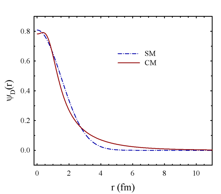
Figure 3: Wave functions of deuteron obtained in the shell model (SM) and cluster model (CM).

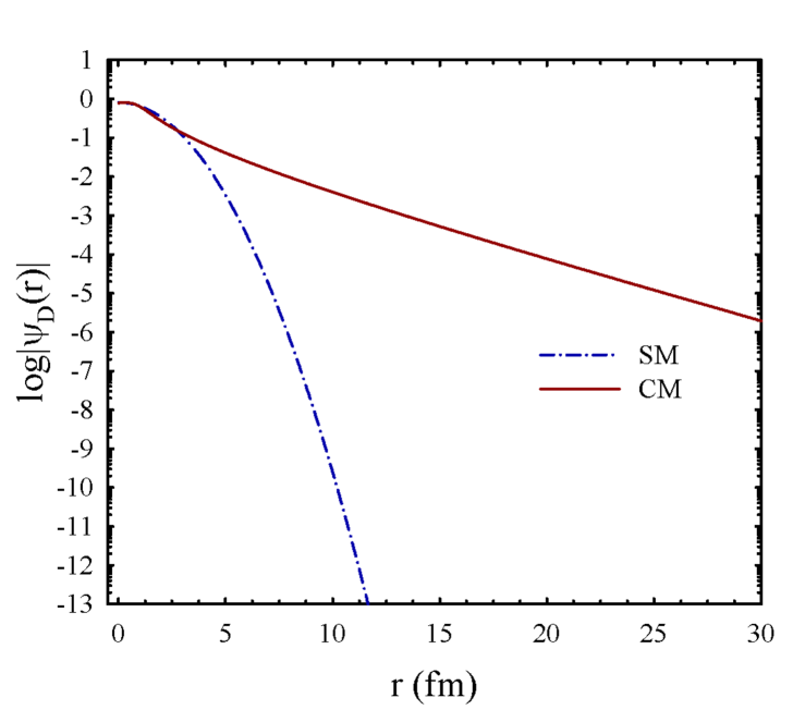
Figure 4: Asymptotic form of the deuteron wave functions constructed in the shell model (SM) and cluster model (CM).

Deuteron form factors calculated within the shell model and cluster model are shown in Figs. 5 and 6.

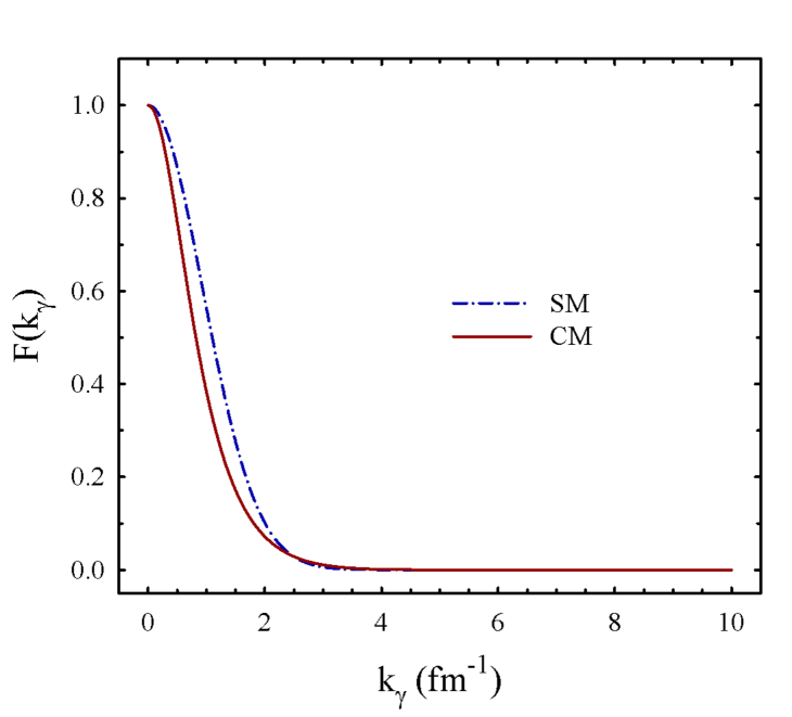
Figure 5: Form factors of deuteron determined in the shell and cluster models

Figure 6: Form factors of deuteron in logarithmic scale calculated in the shell and cluster models

If the zero-range interaction is used to determine wave function of deuteron (43), then the deuteron form factor is (see App. C)

$$F_{1}(\boldsymbol{k}_{\gamma})=\dfrac{2\sqrt{2}\kappa}{k_{\gamma}}\arctan\biggl(\dfrac{k_{\gamma}}{2\sqrt{2}\kappa}\biggr{missing}).$$ (61)

This form factor is shown in Figs. 7.

Figure 7: Form factor $F_{1}$ (in left panel) and square of this form factor $F_{1}^{2}$ (in right panel) at $\kappa=0.325879$ fm^-1.

VI.2 Wave functions of $p+d$ system

In Fig. 8 we display phase shifts of the elastic $p+d$ scattering. One can see that the strongest interaction is observed in the 1/2⁺ state, where the nucleus ³He has a bound state. For energy $E>$100 MeV, all displayed phase shifts are very close to zero. This is an additional indication that potential of the $p+d$ interaction is weak and that the Born approximation can be used for this energy range.

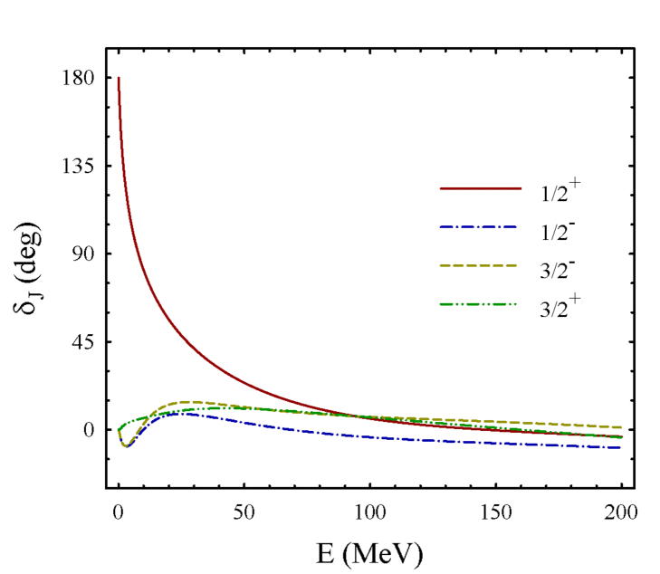
Figure 8: Phase shifts of the elastic $p+d$ scattering, obtained with the MP for different $J^{\pi}$ states

We constructed wave functions  of the continuous spectrum states using diagonalization procedure of the 100$\times$100 matrix of Hamiltonian. Details and justification of this procedure can be found, for example, in Refs. 2015NuPhA.941..121L , 2023UkrJPh..68..3K . Fig. 9 shows wave functions of 1/2⁺ states as a function of distance between proton and deuteron. In Fig. 10 we display wave functions for the 1/2^- state. Note that the states 1/2⁺ and 1/2^- can be connected by dipole transition operator. General features of the displayed wave functions are that they have large amplitude at relatively small distances between clusters ($r<$5 fm) and that they slowly decreasing as $1/r$.

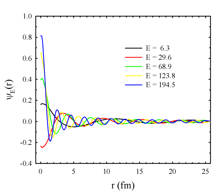
Figure 9: Wave functions of continuous spectrum states  in the 1/2⁺ state of $p+d$ system

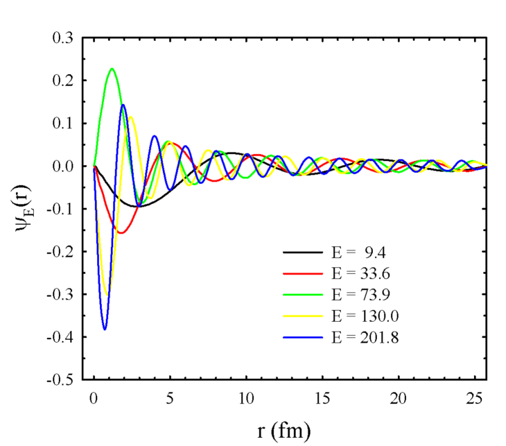
Figure 10: Wave functions of relative motion of proton with respect to deuteron in the 1/2^- state

VI.3 Different NN potentials

In this section we consider how the shape of nucleon-nucleon potential affects phase shifts of the elastic $p+d$ scattering. For this aim we involved in our calculations two new NN potentials. They are the Volkov potential (VP) kn:Volk65 and modified Hasegawa-Nagata potential (MHNP) potMHN1 ; potMHN2 . These potentials alongside with the Minnesota potential are often used in different cluster models. It is demonstrated in Fig. 11, where the even components $V_{31}$ and $V_{13}$ of three nucleon-nucleon potentials are displayed, that the MHNP has the largest repulsive core at small distance between nucleons, the VP has smallest repulsive core and the MP represents intermediate case among three selected potentials.

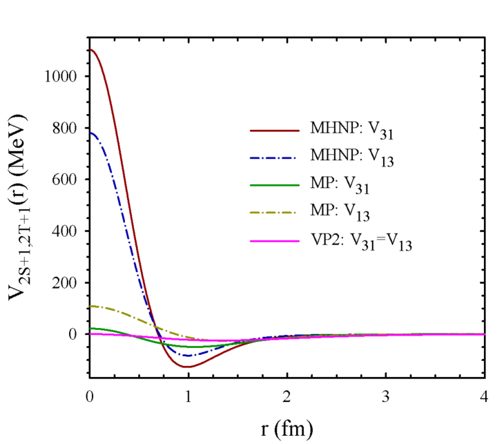
Figure 11: The even components $V_{31}$ and $V_{13}$ of the MHNP, MP and VP nucleon-nucleon potentials as a function of distance between nucleons

In Fig. 12 we display phase shifts of the elastic $p+d$ scattering in the 1/2⁺ state. We can see that the phase shifts slightly depend on the shape of the nucleon-nucleon potentials especially at the energy region $E<$50 MeV. At the energy range 150$<E<$200 differences of phase shifts for different potentials are less than 20 degrees.

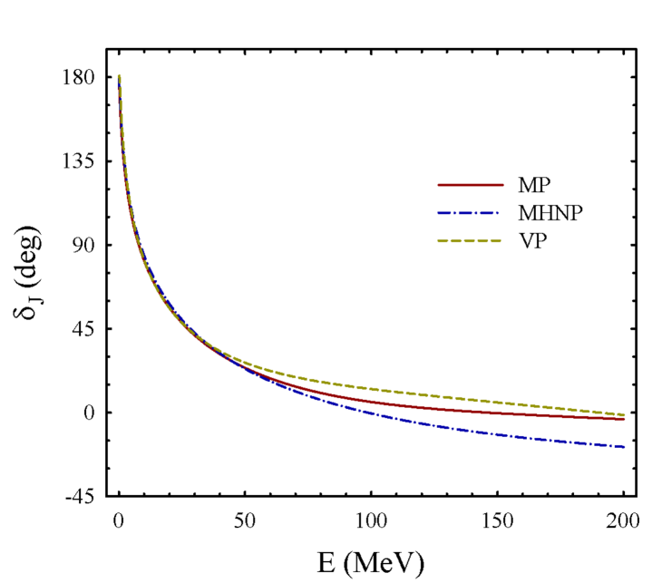
Figure 12: Phase shifts of the $p+d$ scattering in the 1/2⁺ state calculated with three nucleon-nucleon potentials

As a results, wave functions of the elastic $p+d$ scattering obtained with different NN potentials are very close to one other. In Fig. 13 we display wave functions of $p+d$ system for the energy 147 MeV. The noticeable difference of wave functions is observed at small distances $r<$ 1 fm.

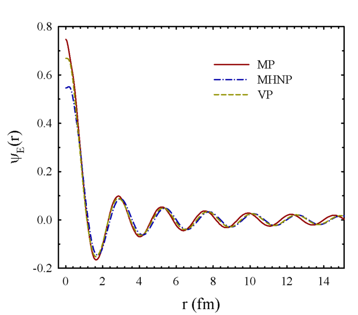
Figure 13: Wave functions of the $p+d$ system at energy 147 MeV obtained with three different nucleon-nucleon potentials

Let us consider the 1/2^- states in ³He and in the $p+d$ elastic scattering. The 1/2^- states can be connected to the 1/2⁺ states by the dipole transition operator. In Fig. 14 we display phase shifts of $p+d$ elastic scattering in the 1/2^- states, calculated with three nucleon-nucleon potentials. At low energy range, phase shifts exhibit resonance-like behavior, when phase shifts rapidly growing with increasing of energy $E$. However, amplitudes of growing are small, besides we estimate that the widths of such resonance states are larger than 20 MeV and their energies are less then 8 MeV. Thus, such states cannot be considered as resonance states.

Figure 14: Phase shifts of the elastic $p+d$ scattering in the 1/2^- state obtained with the MP, MHNP and VP

This conclusion can be partially confirmed by behavior of wave functions in the 1/2^- states. In Fig. 15 we display wave functions obtained with three nucleon-nucleon potentials at the energy $E$=12.7 MeV and in Fig. 16 are shown wave functions for larger value of the energy $E$=147 MeV. As we can see, the wave functions at relatively small and large energies have noticeable maxima at relatively small distances (0.8$<r<$2.5 fm) between proton and deuteron. We may conclude that maxima of wave functions in the 1/2^- state at small distances are due to interplay between effects of nucleon-nucleon and Coulomb interactions from one side and effects of the Pauli principle from another side.

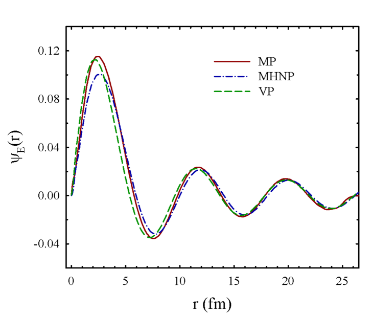
Figure 15: Wave functions of relative motion of proton and deuteron with energy $E$=12.7 MeV and the total angular momentum $J^{\pi}=$1/2^-

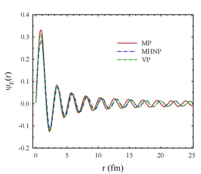
Figure 16: Wave functions of relative motion of proton and deuteron with energy $E$=147 MeV and the total angular momentum $J^{\pi}=$1/2^-

VI.4 Dependence of the bremsstrahlung cross section on the structure of deuteron

We are interesting in question if the bremsstrahlung cross section is dependent on the structure of deuteron. In the previous section we have discussed several forms of the deuteron wave functions. Two of them are presented in analytic form, and one of them is obtained numerically by solving two-body Schrödinger equation with the Minnesota potential. The deuteron wave function of the oscillator shell model, displayed in Eq. (47), allows us in a simple way to study effects of the deuteron structure on the bremsstrahlung cross section. Indeed, this wave function depends on the oscillator length $b$. Recall, that the oscillator length is selected to minimize the ground state energy of deuteron with selected potential. If in Eq. (47) put $b$=0, then we obtain structureless deuteron or, in other words, we disregard of the internal structure of deuteron.

If to suppose existence of such a dependence, it can be small or even not visible for analysis. If this is correct, then it is unclear, if this is not so at other energies. In particular, we would like to find energies, where the spectra are already dependent visibly on the internal structure of deuteron.

Some information about the internal structure of deuteron is included in its form factor, which is presented in the folding and cluster approaches. The matrix element of bremsstrahlung emission in both approaches is defined by Eq. (59) as ($F_{\rm p}=1$), where we will consider form factor of deuteron in folding approach given by Eq. (52) [$Z_{D}=1$, $A_{D}=2$ for deuteron]

$$\begin{array}[]{lllll}F_{D}=&Z_{D}\,\exp{-\displaystyle\frac{1}{4}\,\displaystyle\frac{A_{D}-1}{A_{D}}\,(k,b)^{2}}=\exp{-\displaystyle\frac{1}{8}\,(k,b)^{2}}\end{array}$$ (62)

with the oscillator length $b$.

Results of such calculations at different energies of beam are presented in Fig. 17.

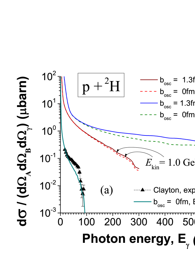
Figure 17: (Color online) Cross sections of bremsstrahlung emission for $p+\isotope[2]{H}$ with included structure of deuteron and without it calculated at energies of beam of 145 MeV ($E_{\rm kin}=98~{}MeV$), 500 MeV ($E_{\rm kin}=333~{}MeV$) and 1.5 GeV ($E_{\rm kin}=1.0~{}GeV$) [Parameters of calculations: cross section is defined in Eq. (58) and then averaged over all angles with exception of photon emission angle $\theta$ used in experiments ($\theta=60^{\circ}$, see also Ref. Nakayama.1992.PRC.v45 , Fig. 5), as non-zero oscillator length for deuteron we choose $b=1.3$ fm, $R_{\rm max}=20000\,{\rm fm}$ and 2500000 intervals are used in the numerical integration; time of computer calculations is 2–4 min for 40 points of each calculated spectrum, kinetic energy $E_{\rm kin}$ of relative motion of proton and deuteron is used in calculations of bremsstrahlung matrix elements, which is $E_{\rm kin}=2/3\cdot E_{\rm beam}$]. Here, experimental data at 145 MeV of beam energy given by black triangles are extracted from Ref. Clayton.1992.PRC.p1810 .

From such results we conclude the following.

1. Difference between cross sections calculated with included structure of deuteron and without it at the same beam energy becomes visible and stable at higher energy of beam (larger 500 MeV).

2. Calculation with realistic wave functions (with included structure of deuteron) gives larger cross section of bremsstrahlung than cross section without inclusion of structure of deuteron.

3. Experiment Clayton.1992.PRC.p1810 at used beam energy of 145 MeV is not effective for such a study (it is demonstrated by cross sections at 1.5 GeV in comparison with cross section at 145 MeV in this figure). At the same time, possible new measurement of bremsstrahlung cross sections but at higher energies (about 0.5–1.5 GeV of beam energy) will allow to extract information about structure of deuteron (realistic oscillator length, and wave function).

4. More precise information about structure of deuteron can be obtained if to organize unified experiments in measurement of bremsstrahlung cross section at two different energies of beam (for example, at 145 MeV and 500 MeV). Then, our model will estimate ratio between two bremsstrahlung cross sections at such energies and provide value about realistic oscillator length with high precision.

VI.5 Dependence of bremsstrahlung cross section on new form factor of deuteron

Now we will analyze how much the spectrum is changed if to use new form factor of deuteron instead of previous calculations. So, we have the matrix element in form (59) as with form factor of deuteron given by Eq. (61). Note that this form factor of deuteron does not include the oscillator length. Results of such calculations with new form factor are presented in Fig. 18.

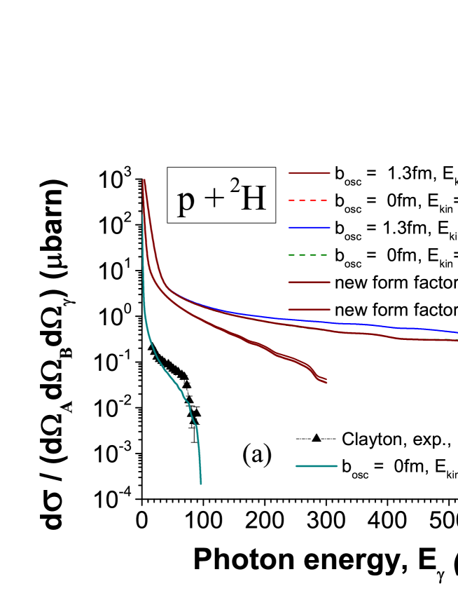
Figure 18: (Color online) Cross sections of bremsstrahlung emission for $p+\isotope[2]{H}$ with included new form factor calculated at energies of beam of 145 MeV ($E_{\rm kin}=98~{}MeV$), 500 MeV ($E_{\rm kin}=333~{}MeV$) and 1.5 GeV ($E_{\rm kin}=1.0~{}GeV$) [Parameters of calculations: cross section is defined in Eq. (58), matrix element is defined in Eq. (59), as non-zero oscillator length for deuteron we choose $b=1.3$ fm, $R_{\rm max}=20000\,{\rm fm}$ and 2500000 intervals are used in the numerical integration; time of computer calculations is 2–4 min for 40 points of each calculated spectrum, kinetic energy $E_{\rm kin}$ of relative motion of proton and deuteron is used in calculations of bremsstrahlung matrix elements, which is $E_{\rm kin}=2/3\cdot E_{\rm beam}$]. Here, experimental data at 145 MeV of beam energy given by black triangles are extracted from Ref. Clayton.1992.PRC.p1810 .

From these calculations one can see that inclusion of new form factor reduces full cross section a little. But, general dependence of the cross section on this form of form factor is observed at higher energies.

VII Conclusions and perspectives

In this paper we investigated emission of bremsstrahlung photons in the scattering of protons off deuterons on the fully cluster basis in a wide region of the beam energy from low energies till 1.5 GeV. To realize this investigations, we developed a new model. On the basis of such a model we obtain the following results:

• It is demonstrated that the matrix elements of bremsstrahlung emission in the deuteron-proton scattering in the three-cluster formalism coincides with the corresponding matrix elements in the folding approximation given in Ref. Maydanyuk_Vasilevsky.2023.PRC .

• Formalism of the model includes form factor of a deuteron which affects behavior of bremsstrahlung cross sections and reflects the structure of deuteron and influence of parameters of nucleon-nucleon interactions. This gives possibility to investigate structure of nuclei and properties of interactions from analysis of bremsstrahlung cross sections.

• We studied dependence of the bremsstrahlung cross section on structure of deuteron. We find that the oscillator length $b$, related to the shell-model description of the deuteron, is convenient parameter for such a study. Analysis of dependence of the cross section on such a parameter shows the following. At beam energies used at experiment Clayton.1992.PRC.p1810 the cross section is not sensitive visibly on variations of oscillator length, i.e. on the internal structure of deuteron. However, stable difference between cross sections calculated at zero and non-zero oscillator lengths at the same beam energy is observed at higher energy of beam (larger 500 MeV). The spectrum is increased at increasing of the oscillator length inside the full energy region of the emitted photons. However, the usage of new the deuteron form factor in the cluster formalism [see Eq. (61)] reduces the bremsstrahlung cross section a little.

• More precise information about structure of deuteron can be obtained if to organize unified new experiments in measurement of bremsstrahlung cross section at two different energies of beam (for example, at 145 MeV and 500 MeV or above). Then, our model will estimate ratio between two bremsstrahlung cross sections at such energies and provide information about realistic value of the oscillator length with high precision.

As a perspective, we see that formalism of our model provides strict basis for description of the deuteron-proton scattering and emission of virtual photons in study of dilepton productions in the deuteron-proton scattering (see, for example, Refs. Ernst.1998.PRC ; Wilson.1998.PRC ). This can be interesting for further investigations and applications.

Appendix A Calculation of operator of bremsstrahlung emission in three-cluster model

In this Appendix we will calculate operator of emission of bremsstrahlung photons in three-cluster formalism. We fix position of nucleons. We assume that vector $\mathbf{r}$ measures the distance between proton and neutron which form a deuteron. We also assume that $\mathbf{r}_{1}$ is a coordinate of the first proton and $\mathbf{r}_{2}$ is a coordinate of a neutron. Vector $\mathbf{r}_{3}$ determines the location of the second proton. Starting from Eq. (1), this operator is obtained the following form:

$$\widehat{H}_{e}\left(\mathbf{k}_{\gamma},\mathbf{\varepsilon}^{(\alpha)}\right)=\frac{1}{2}\frac{e\hbar}{m_{N}c}\left[\widehat{\mathbf{\pi}}_{1}^{\ast}\mathbf{A}^{\ast}\left(1\right)+\mathbf{A}^{\ast}\left(1\right)\widehat{\mathbf{\pi}}_{1}^{\ast}+\widehat{\mathbf{\pi}}_{3}^{\ast}\mathbf{A}^{\ast}\left(3\right)+\mathbf{A}^{\ast}\left(3\right)\widehat{\mathbf{\pi}}_{3}^{\ast}\right]$$

$$=\frac{1}{2}\frac{e\hbar}{m_{N}c}\left\{\widehat{\mathbf{\pi}}_{1}^{\ast}\mathbf{\varepsilon}^{(\alpha)}\exp\left\{-i\left(\mathbf{k}_{\gamma}\mathbf{\rho}_{1}\right)\right\}+\mathbf{\varepsilon}^{(\alpha)}\exp\left\{-i\left(\mathbf{k}_{\gamma}\mathbf{\rho}_{1}\right)\right\}\widehat{\mathbf{\pi}}_{1}^{\ast}\right.$$

$$+\left.\widehat{\mathbf{\pi}}_{3}^{\ast}\mathbf{\varepsilon}^{(\alpha)}\exp\left\{-i\left(\mathbf{k}_{\gamma}\mathbf{\rho}_{3}\right)\right\}+\mathbf{\varepsilon}^{(\alpha)}\exp\left\{-i\left(\mathbf{k}_{\gamma}\mathbf{\rho}_{3}\right)\right\}\widehat{\mathbf{\pi}}_{3}^{\ast}\right\}$$

$$=\frac{1}{2}\frac{e\hbar}{m_{N}c}\left\{\left(\mathbf{\varepsilon}^{(\alpha)}\widehat{\mathbf{\pi}}_{1}^{\ast}\right)\exp\left\{-i\frac{1}{\sqrt{2}}\left(\mathbf{k}_{\gamma}\mathbf{r}\right)\mathbf{+}i\frac{1}{\sqrt{6}}\left(\mathbf{k}_{\gamma}\mathbf{q}\right)\right\}\right.$$

$$+\exp\left\{-i\frac{1}{\sqrt{2}}\left(\mathbf{k}_{\gamma}\mathbf{r}\right)\mathbf{+}i\frac{1}{\sqrt{6}}\left(\mathbf{k}_{\gamma}\mathbf{q}\right)\right\}\left(\mathbf{\varepsilon}^{(\alpha)}\widehat{\mathbf{\pi}}_{1}^{\ast}\right)$$

$$+\left.\left(\mathbf{\varepsilon}^{(\alpha)}\widehat{\mathbf{\pi}}_{3}^{\ast}\right)\exp\left\{-i\sqrt{\frac{2}{3}}\left(\mathbf{k}_{\gamma}\mathbf{q}\right)\right\}+\exp\left\{-i\sqrt{\frac{2}{3}}\left(\mathbf{k}_{\gamma}\mathbf{q}\right)\right\}\left(\mathbf{\varepsilon}^{(\alpha)}\widehat{\mathbf{\pi}}_{3}^{\ast}\right)\right\}$$

and then

$$\widehat{H}_{e}\left(\mathbf{k}_{\gamma},\mathbf{\varepsilon}^{(\alpha)}\right)$$

$$=\frac{1}{2}\frac{e\hbar}{m_{N}c}\left\{\left(\mathbf{\varepsilon}^{(\alpha)},\frac{1}{\sqrt{2}}\mathbf{\pi}_{\mathbf{r}}^{\ast}\mathbf{-}\frac{1}{\sqrt{6}}\mathbf{\pi}_{\mathbf{q}}^{\ast}\right)\exp\left\{-i\frac{1}{\sqrt{2}}\left(\mathbf{k}_{\gamma}\mathbf{r}\right)\mathbf{+}i\frac{1}{\sqrt{6}}\left(\mathbf{k}_{\gamma}\mathbf{q}\right)\right\}\right.$$

$$+\exp\left\{-i\frac{1}{\sqrt{2}}\left(\mathbf{k}_{\gamma}\mathbf{r}\right)\mathbf{+}i\frac{1}{\sqrt{6}}\left(\mathbf{k}_{\gamma}\mathbf{q}\right)\right\}\left(\mathbf{\varepsilon}^{(\alpha)},\frac{1}{\sqrt{2}}\mathbf{\pi}_{\mathbf{r}}^{\ast}\mathbf{-}\frac{1}{\sqrt{6}}\mathbf{\pi}_{\mathbf{q}}^{\ast}\right)$$

$$+\left.\sqrt{\frac{2}{3}}\left(\mathbf{\varepsilon}^{(\alpha)}\mathbf{\pi}_{\mathbf{q}}^{\ast}\right)\exp\left\{-i\sqrt{\frac{2}{3}}\left(\mathbf{k}_{\gamma}\mathbf{q}\right)\right\}+\sqrt{\frac{2}{3}}\exp\left\{-i\sqrt{\frac{2}{3}}\left(\mathbf{k}_{\gamma}\mathbf{q}\right)\right\}\left(\mathbf{\varepsilon}^{(\alpha)}\mathbf{\pi}_{\mathbf{q}}^{\ast}\right)\right\}$$

Collecting similar terms we obtain

$$\widehat{H}_{e}\left(\mathbf{k}_{\gamma},\mathbf{\varepsilon}^{(\alpha)}\right)=\frac{1}{2}\frac{e\hbar}{m_{N}c}\left\{\left(\mathbf{\varepsilon}^{(\alpha)},\frac{1}{2}\mathbf{k}_{\gamma}\mathbf{+}\frac{1}{6}\mathbf{k}_{\gamma}\right)\exp\left\{-i\frac{1}{\sqrt{2}}\left(\mathbf{k}_{\gamma}\mathbf{r}\right)+i\frac{1}{\sqrt{6}}\left(\mathbf{k}_{\gamma}\mathbf{q}\right)\right\}\right.$$

$$+2\exp\left\{-i\frac{1}{\sqrt{2}}\left(\mathbf{k}_{\gamma}\mathbf{r}\right)\mathbf{+}i\frac{1}{\sqrt{6}}\left(\mathbf{k}_{\gamma}\mathbf{q}\right)\right\}\left(\mathbf{\varepsilon}^{(\alpha)},\frac{1}{\sqrt{2}}\mathbf{\pi}_{\mathbf{r}}^{\ast}\mathbf{-}\frac{1}{\sqrt{6}}\mathbf{\pi}_{\mathbf{q}}^{\ast}\right)$$

$$+\sqrt{\frac{2}{3}}\left(\mathbf{\varepsilon}^{(\alpha)}i\left[-i\sqrt{\frac{2}{3}}\mathbf{k}_{\gamma}\right]\right)\exp\left\{-i\sqrt{\frac{2}{3}}\left(\mathbf{k}_{\gamma}\mathbf{q}\right)\right\}$$

$$+\left.2\sqrt{\frac{2}{3}}\exp\left\{-i\sqrt{\frac{2}{3}}\left(\mathbf{k}_{\gamma}\mathbf{q}\right)\right\}\left(\mathbf{\varepsilon}^{(\alpha)}\mathbf{\pi}_{\mathbf{q}}^{\ast}\right)\right\}$$

or

$$\widehat{H}_{e}\left(\mathbf{k}_{\gamma},\mathbf{\varepsilon}^{(\alpha)}\right)=\frac{1}{2}\frac{e\hbar}{m_{N}c}\left\{\frac{2}{3}\left(\mathbf{\varepsilon}^{(\alpha)},\mathbf{k}_{\gamma}\right)\exp\left\{-i\frac{1}{\sqrt{2}}\left(\mathbf{k}_{\gamma}\mathbf{r}\right)\mathbf{+}i\frac{1}{\sqrt{6}}\left(\mathbf{k}_{\gamma}\mathbf{q}\right)\right\}\right.$$

$$+2\exp\left\{-i\frac{1}{\sqrt{2}}\left(\mathbf{k}_{\gamma}\mathbf{r}\right)\mathbf{+}i\frac{1}{\sqrt{6}}\left(\mathbf{k}_{\gamma}\mathbf{q}\right)\right\}\left(\mathbf{\varepsilon}^{(\alpha)},\frac{1}{\sqrt{2}}\mathbf{\pi}_{\mathbf{r}}^{\ast}\mathbf{-}\frac{1}{\sqrt{6}}\mathbf{\pi}_{\mathbf{q}}^{\ast}\right)$$

$$+\frac{2}{3}\left(\mathbf{\varepsilon}^{(\alpha)}\mathbf{k}_{\gamma}\right)\exp\left\{-i\sqrt{\frac{2}{3}}\left(\mathbf{k}_{\gamma}\mathbf{q}\right)\right\}$$

$$+\left.2\sqrt{\frac{2}{3}}\exp\left\{-i\sqrt{\frac{2}{3}}\left(\mathbf{k}_{\gamma}\mathbf{q}\right)\right\}\left(\mathbf{\varepsilon}^{(\alpha)}\mathbf{\pi}_{\mathbf{q}}^{\ast}\right)\right\}$$

or

$$\widehat{H}_{e}\left(\mathbf{k}_{\gamma},\mathbf{\varepsilon}^{(\alpha)}\right)=\frac{1}{2}\frac{e\hbar}{m_{N}c}\left\{\frac{2}{3}\left(\mathbf{\varepsilon}^{(\alpha)},\mathbf{k}_{\gamma}\right)\exp\left\{-i\frac{1}{\sqrt{2}}\left(\mathbf{k}_{\gamma}\mathbf{r}\right)\mathbf{+}i\frac{1}{\sqrt{6}}\left(\mathbf{k}_{\gamma}\mathbf{q}\right)\right\}\right.$$

$$+\frac{2}{3}\left(\mathbf{\varepsilon}^{(\alpha)}\mathbf{k}_{\gamma}\right)\exp\left\{-i\sqrt{\frac{2}{3}}\left(\mathbf{k}_{\gamma}\mathbf{q}\right)\right\}$$

$$+2\exp\left\{-i\frac{1}{\sqrt{2}}\left(\mathbf{k}_{\gamma}\mathbf{r}\right)\mathbf{+}i\frac{1}{\sqrt{6}}\left(\mathbf{k}_{\gamma}\mathbf{q}\right)\right\}\left(\mathbf{\varepsilon}^{(\alpha)},\frac{1}{\sqrt{2}}\mathbf{\pi}_{\mathbf{r}}^{\ast}\mathbf{-}\frac{1}{\sqrt{6}}\mathbf{\pi}_{\mathbf{q}}^{\ast}\right)$$

$$+\left.2\sqrt{\frac{2}{3}}\exp\left\{-i\sqrt{\frac{2}{3}}\left(\mathbf{k}_{\gamma}\mathbf{q}\right)\right\}\left(\mathbf{\varepsilon}^{(\alpha)},\mathbf{\pi}_{\mathbf{q}}^{\ast}\right)\right\}$$

Final form of the operator

$$\widehat{H}_{e}\left(\mathbf{k}_{\gamma},\mathbf{\varepsilon}^{(\alpha)}\right)=\frac{1}{2}\frac{e\hbar}{m_{N}c}\left\{\frac{2}{3}\left(\mathbf{\varepsilon}^{(\alpha)},\mathbf{k}_{\gamma}\right)\exp\left\{-i\frac{1}{\sqrt{2}}\left(\mathbf{k}_{\gamma}\mathbf{r}\right)\mathbf{+}i\frac{1}{\sqrt{6}}\left(\mathbf{k}_{\gamma}\mathbf{q}\right)\right\}\right.$$ (63)

$$+\frac{2}{\sqrt{2}}\exp\left\{-i\frac{1}{\sqrt{2}}\left(\mathbf{k}_{\gamma}\mathbf{r}\right)\mathbf{+}\right\}\exp\left\{\mathbf{+}i\frac{1}{\sqrt{6}}\left(\mathbf{k}_{\gamma}\mathbf{q}\right)\right\}\left(\mathbf{\varepsilon}^{(\alpha)},\mathbf{\pi}_{\mathbf{r}}^{\ast}\right)$$

$$+\frac{2}{3}\left(\mathbf{\varepsilon}^{(\alpha)}\mathbf{k}_{\gamma}\right)\exp\left\{-i\sqrt{\frac{2}{3}}\left(\mathbf{k}_{\gamma}\mathbf{q}\right)\right\}$$

$$\mathbf{-}\sqrt{\frac{2}{3}}\exp\left\{-i\frac{1}{\sqrt{2}}\left(\mathbf{k}_{\gamma}\mathbf{r}\right)\right\}\exp\left\{\mathbf{+}i\frac{1}{\sqrt{6}}\left(\mathbf{k}_{\gamma}\mathbf{q}\right)\right\}\left(\mathbf{\varepsilon}^{(\alpha)},\mathbf{\pi}_{\mathbf{q}}^{\ast}\right)$$

$$+\left.2\sqrt{\frac{2}{3}}\exp\left\{-i\sqrt{\frac{2}{3}}\left(\mathbf{k}_{\gamma}\mathbf{q}\right)\right\}\left(\mathbf{\varepsilon}^{(\alpha)},\mathbf{\pi}_{\mathbf{q}}^{\ast}\right)\right\}$$

or by taking into account that $\left(\mathbf{\varepsilon}^{(\alpha)},\mathbf{k}_{\gamma}\right)=0$, we obtain

$$\widehat{H}_{e}\left(\mathbf{k}_{\gamma},\mathbf{\varepsilon}^{(\alpha)}\right)=\frac{1}{2}\frac{e\hbar}{m_{N}c}\left\{{}\right.$$ (64)

$$+\frac{2}{\sqrt{2}}\exp\left\{-i\frac{1}{\sqrt{2}}\left(\mathbf{k}_{\gamma}\mathbf{r}\right)\right\}\left(\mathbf{\varepsilon}^{(\alpha)},\mathbf{\pi}_{\mathbf{r}}^{\ast}\right)\exp\left\{i\frac{1}{\sqrt{6}}\left(\mathbf{k}_{\gamma}\mathbf{q}\right)\right\}$$

$$\mathbf{-}\sqrt{\frac{2}{3}}\exp\left\{-i\frac{1}{\sqrt{2}}\left(\mathbf{k}_{\gamma}\mathbf{r}\right)\right\}\exp\left\{i\frac{1}{\sqrt{6}}\left(\mathbf{k}_{\gamma}\mathbf{q}\right)\right\}\left(\mathbf{\varepsilon}^{(\alpha)},\mathbf{\pi}_{\mathbf{q}}^{\ast}\right)$$

$$+\left.2\sqrt{\frac{2}{3}}\exp\left\{-i\sqrt{\frac{2}{3}}\left(\mathbf{k}_{\gamma}\mathbf{q}\right)\right\}\left(\mathbf{\varepsilon}^{(\alpha)},\mathbf{\pi}_{\mathbf{q}}^{\ast}\right)\right\}.$$

Appendix B Calculations of integrals

B.1 A general case

In this Appendix we calculate integrals (21):

$$\begin{array}[]{lllll}\vspace{0.5mm}\mathbf{I}_{1}=\biggl{\langle}\>\Phi_{f}(\mathbf{r})\;\biggl{|}\,e^{-i\,\mathbf{k}_{\gamma}\mathbf{r}}\;\mathbf{\displaystyle\frac{d}{dr}}\biggr{|}\>\Phi_{i}(\mathbf{r})\>\biggr{\rangle}_{\mathbf{r}},\\ \vspace{0.5mm}I_{2}=\Bigl{\langle}\Phi_{f}(\mathbf{r})\;\Bigl{|}\,e^{i\,c_{p}\,\mathbf{k_{\gamma}}\mathbf{r}}\,\Bigr{|}\,\Phi_{i}(\mathbf{r})\>\Bigr{\rangle}_{\mathbf{r}},\\ \vspace{0.5mm}I_{3}=\Bigl{\langle}\Phi_{f}(\mathbf{r})\;\Bigl{|}\,e^{-i\,c_{A}\,\mathbf{k_{\gamma}}\mathbf{r}}\,\Bigr{|}\,\Phi_{i}(\mathbf{r})\>\Bigr{\rangle}_{\mathbf{r}},\\ I_{4}=\Bigl{\langle}\Phi_{f}(\mathbf{r})\;\Bigl{|}\,e^{-i\,c_{A}\,\mathbf{k_{\gamma}}\mathbf{r}}\,V(\mathbf{r})\,\Bigr{|}\,\Phi_{i}(\mathbf{r})\>\Bigr{\rangle}_{\mathbf{r}}.\end{array}$$ (65)

Here, to two integrals in Eqs. (21) we have added two new types of integrals else, which are used in calculations in other problems of bremsstrahlung emission. $V(\mathbf{r})$ is arbitrary potential function.

We apply multipole expansion of wave function of photons, following to formalism in Sect. D in Ref. Maydanyuk.2012.PRC [see Eqs. (29)–(31) and (24)–(28) in that paper]. Here, we obtain the following formulas for matrix elements:

$$\begin{array}[]{ll}\vspace{1mm}\Bigl{<}k_{f}\Bigl{|}\,e^{-i\mathbf{k_{\gamma}r}}\,\Bigr{|}\,k_{i}\Bigr{>}_{\mathbf{r}}=\sqrt{\displaystyle\frac{\pi}{2}}\>\displaystyle\sum\limits_{l_{\gamma}=1}\,(-i)^{l_{\gamma}}\,\sqrt{2l_{\gamma}+1}\;\displaystyle\sum\limits_{\mu=\pm 1}\Bigl{[}\mu\,\tilde{p}_{l_{\gamma}\mu}^{M}-i\,\tilde{p}_{l_{\gamma}\mu}^{E}\Bigr{]},\\ \biggl{<}k_{f}\biggl{|}\,e^{-i\mathbf{k_{\gamma}r}}\displaystyle\frac{\partial}{\partial\mathbf{r}}\,\biggr{|}\,k_{i}\biggr{>}_{\mathbf{r}}=\sqrt{\displaystyle\frac{\pi}{2}}\>\displaystyle\sum\limits_{l_{\gamma}=1}\,(-i)^{l_{\gamma}}\,\sqrt{2l_{\gamma}+1}\;\displaystyle\sum\limits_{\mu=\pm 1}\mbox{\boldmath$\xi$}_{\mu}\,\mu\,\times\Bigl{[}p_{l_{\gamma}\mu}^{M}-i\mu\>p_{l_{\gamma}\mu}^{E}\Bigr{]}.\end{array}$$ (66)

On the basis of these formulas, we write solutions for integrals (for simplicity, we study case of $l_{i}=0$).

According to the second formula in Eqs. (66), the first integral is

$$\begin{array}[]{ll}\mathbf{I}_{1}=\biggl{<}\Phi_{f}\biggl{|}\,e^{-i\mathbf{k_{\gamma}r}}\displaystyle\frac{\partial}{\partial\mathbf{r}}\,\biggr{|}\,\Phi_{i}\biggr{>}_{\mathbf{r}}=\sqrt{\displaystyle\frac{\pi}{2}}\>\displaystyle\sum\limits_{l_{\gamma}=1}\,(-i)^{l_{\gamma}}\,\sqrt{2l_{\gamma}+1}\;\displaystyle\sum\limits_{\mu=\pm 1}\mbox{\boldmath$\xi$}_{\mu}\,\mu\,\times\Bigl{[}p_{l_{\gamma}\mu}^{M}-i\mu\>p_{l_{\gamma}\mu}^{E}\Bigr{]},\end{array}$$ (67)

where [see Eqs. (38) at $l_{i}=0$ in Ref. Maydanyuk.2012.PRC ]

$$\begin{array}[]{lcl}\vspace{3mm}p_{l_{\gamma}\mu}^{M}&=&-I_{M}(0,l_{f},l_{\gamma},1,\mu)\cdot J_{1}(0,l_{f},l_{\gamma}),\\ \vspace{1mm}p_{l_{\gamma}\mu}^{E}&=&\sqrt{\displaystyle\frac{l_{\gamma}+1}{2l_{\gamma}+1}}\cdot I_{E}(0,l_{f},l_{\gamma},1,l_{\gamma}-1,\mu)\cdot J_{1}(0,l_{f},l_{\gamma}-1)\;-\\ &-&\sqrt{\displaystyle\frac{l_{\gamma}}{2l_{\gamma}+1}}\cdot I_{E}(0,l_{f},l_{\gamma},1,l_{\gamma}+1,\mu)\cdot J_{1}(0,l_{f},l_{\gamma}+1)\end{array}$$ (68)

and [see Eqs. (39) in Ref. Maydanyuk.2012.PRC ]

$$\begin{array}[]{ccl}J_{1}(l_{i},l_{f},n)&=&\displaystyle\int\limits^{+\infty}_{0}\displaystyle\frac{dR_{i}(r,l_{i})}{dr}\>R^{*}_{f}(l_{f},r)\,j_{n}(k_{\gamma}r)\;r^{2}dr.\end{array}$$ (69)

For the other integrals from Eqs. (65) one can get similar solutions [those are directly derived from the first expansion in Eqs. (66), where the other corresponding radial integrals should be used]:

$$\begin{array}[]{lllll}\vspace{0.5mm}I_{2}=\Bigl{\langle}\Phi_{f}\;\Bigl{|}\,e^{i\,c_{p}\,\mathbf{k_{\gamma}}\mathbf{r}}\,\Bigr{|}\,\Phi_{i}\>\Bigr{\rangle}_{\mathbf{r}}=\par\sqrt{\displaystyle\frac{\pi}{2}}\>\displaystyle\sum\limits_{l_{\gamma}=1}\,(-i)^{l_{\gamma}}\,\sqrt{2l_{\gamma}+1}\;\displaystyle\sum\limits_{\mu=\pm 1}\Bigl{[}\mu\,\tilde{p}_{l_{\gamma}\mu}^{M}(-c_{p})-i\,\tilde{p}_{l_{\gamma}\mu}^{E}(-c_{p})\Bigr{]},\\ \vspace{0.5mm}I_{3}=\Bigl{\langle}\Phi_{f}\;\Bigl{|}\,e^{-i\,c_{A}\,\mathbf{k_{\gamma}}\mathbf{r}}\,\Bigr{|}\,\Phi_{i}\>\Bigr{\rangle}_{\mathbf{r}}=\sqrt{\displaystyle\frac{\pi}{2}}\>\displaystyle\sum\limits_{l_{\gamma}=1}\,(-i)^{l_{\gamma}}\,\sqrt{2l_{\gamma}+1}\;\displaystyle\sum\limits_{\mu=\pm 1}\Bigl{[}\mu\,\tilde{p}_{l_{\gamma}\mu}^{M}(c_{A})-i\,\tilde{p}_{l_{\gamma}\mu}^{E}(c_{A})\Bigr{]},\\ I_{4}=\Bigl{\langle}\Phi_{f}\;\Bigl{|}\,e^{-i\,c_{A}\,\mathbf{k_{\gamma}}\mathbf{r}}\,V(\mathbf{r})\,\Bigr{|}\,\Phi_{i}\>\Bigr{\rangle}_{\mathbf{r}}=\par\sqrt{\displaystyle\frac{\pi}{2}}\>\displaystyle\sum\limits_{l_{\gamma}=1}\,(-i)^{l_{\gamma}}\,\sqrt{2l_{\gamma}+1}\;\displaystyle\sum\limits_{\mu=\pm 1}\Bigl{[}\mu\,\breve{p}_{l_{\gamma}\mu}^{M}(c_{A})-i\,\breve{p}_{l_{\gamma}\mu}^{E}(c_{A})\Bigr{]},\end{array}$$ (70)

where [see solutions (40) at $l_{i}=0$ in Ref. Maydanyuk.2012.PRC for $\tilde{p}_{l_{\gamma}\mu}^{M}$, $\tilde{p}_{l_{\gamma}\mu}^{E}$, Eqs. (F14) and (F26) in Ref. Maydanyuk_Zhang_Zou.2019.PRC.microscopy for all matrix elements]

$$\begin{array}[]{llll}\vspace{3mm}\tilde{p}_{l_{\gamma}\mu}^{M}(c)=\tilde{I}\,(0,l_{f},l_{\gamma},l_{\gamma},\mu)\cdot\tilde{J}\,(c,0,l_{f},l_{\gamma}),\\ \vspace{3mm}\tilde{p}_{l_{\gamma}\mu}^{E}(c)=\sqrt{\displaystyle\frac{l_{\gamma}+1}{2l_{\gamma}+1}}\tilde{I}\,(0,l_{f},l_{\gamma},l_{\gamma}-1,\mu)\cdot\tilde{J}\,(c,0,l_{f},l_{\gamma}-1)\;-\sqrt{\displaystyle\frac{l_{\gamma}}{2l_{\gamma}+1}}\tilde{I}\,(0,l_{f},l_{\gamma},l_{\gamma}+1,\mu)\cdot\tilde{J}\,(c,0,l_{f},l_{\gamma}+1),\\ \vspace{3mm}\breve{p}_{l_{\gamma}\mu}^{M}(c_{A})=\tilde{I}\,(0,l_{f},l_{\gamma},l_{\gamma},\mu)\cdot\breve{J}\,(c_{A},0,l_{f},l_{\gamma}),\\ \breve{p}_{l_{\gamma}\mu}^{E}(c_{A})=\sqrt{\displaystyle\frac{l_{\gamma}+1}{2l_{\gamma}+1}}\tilde{I}\,(0,l_{f},l_{\gamma},l_{\gamma}-1,\mu)\cdot\breve{J}\,(c_{A},0,l_{f},l_{\gamma}-1)\;-\sqrt{\displaystyle\frac{l_{\gamma}}{2l_{\gamma}+1}}\tilde{I}\,(0,l_{f},l_{\gamma},l_{\gamma}+1,\mu)\cdot\breve{J}\,(c_{A},0,l_{f},l_{\gamma}+1)\end{array}$$ (71)

and [see solutions (41) in Ref. Maydanyuk.2012.PRC for $\tilde{J}$ and corresponding angular integral, Eqs. (F13) and (F21) in Ref. Maydanyuk_Zhang_Zou.2019.PRC.microscopy for all matrix elements]

$$\begin{array}[]{ccl}\tilde{J}\,(c,l_{i},l_{f},n)&=&\displaystyle\int\limits^{+\infty}_{0}R_{i}(r)\,R^{*}_{f}(l,r)\,j_{n}(c\,k_{\gamma}r)\;r^{2}dr,\\ \breve{J}\,(c_{A},l_{i},l_{f},n)&=&\displaystyle\int\limits^{+\infty}_{0}R_{i}(r)\,R^{*}_{l,f}(r)\,V(\mathbf{r})\,j_{n}(c_{A}\,kr)\;r^{2}dr.\end{array}$$ (72)

B.2 Linear and circular polarizations of the photon emitted

Rewrite vectors of linear polarization $\mbox{\boldmath$\varepsilon$}^{(\alpha)}$ through vectors of circular polarization $\mathbf{\xi}_{\mu}$ with opposite directions of rotation (see Ref. Eisenberg.1973 , (2.39), p. 42):

$$\begin{array}[]{ccc}\mathbf{\xi}_{-1}=\displaystyle\frac{1}{\sqrt{2}}\,\bigl{(}\mbox{\boldmath$\varepsilon$}^{(1)}-i\mbox{\boldmath$\varepsilon$}^{(2)}\bigr{)},&\mathbf{\xi}_{+1}=-\displaystyle\frac{1}{\sqrt{2}}\,\bigl{(}\mbox{\boldmath$\varepsilon$}^{(1)}+i\mbox{\boldmath$\varepsilon$}^{(2)}\bigr{)},&\mathbf{\xi}_{0}=\mbox{\boldmath$\varepsilon$}^{(3)}.\end{array}$$ (73)

where

$$\begin{array}[]{ccc}h_{\pm}=\mp\displaystyle\frac{1\pm i}{\sqrt{2}},&h_{-1}+h_{+1}=-i\sqrt{2},&\sum\limits_{\alpha=1,2}\mbox{\boldmath$\varepsilon$}^{(\alpha),*}=h_{-1}\mathbf{\xi}_{-1}^{*}+h_{+1}\mathbf{\xi}_{+1}^{*}.\end{array}$$ (74)

We have (in Coulomb gauge at $\mbox{\boldmath$\varepsilon$}^{(3)}=0$)

$$\begin{array}[]{cc}\mbox{\boldmath$\varepsilon$}^{(1)}=\displaystyle\frac{1}{\sqrt{2}}\,\bigl{(}\mbox{\boldmath$\xi$}_{-1}-\mbox{\boldmath$\xi$}_{+1}\bigr{)},&\mbox{\boldmath$\varepsilon$}^{(2)}=\displaystyle\frac{i}{\sqrt{2}}\,\bigl{(}\mbox{\boldmath$\xi$}_{-1}+\mbox{\boldmath$\xi$}_{+1}\bigr{)},\end{array}$$ (75)

$$\begin{array}[]{ccc}\displaystyle\sum\limits_{\mu=\pm 1}\xi_{\mu}^{*}\cdot\xi_{\mu}=\displaystyle\frac{1}{2}\,\bigl{(}\mbox{\boldmath$\varepsilon$}^{(1)}-i\mbox{\boldmath$\varepsilon$}^{(2)}\bigr{)}\,\bigl{(}\mbox{\boldmath$\varepsilon$}^{(1)}-i\mbox{\boldmath$\varepsilon$}^{(2)}\bigr{)}^{*}+\displaystyle\frac{1}{2}\,\bigl{(}\mbox{\boldmath$\varepsilon$}^{(1)}+i\mbox{\boldmath$\varepsilon$}^{(2)}\bigr{)}\,\bigl{(}\mbox{\boldmath$\varepsilon$}^{(1)}+i\mbox{\boldmath$\varepsilon$}^{(2)}\bigr{)}^{*}=2.\end{array}$$ (76)

Also we will find vectorial products of vectors $\mbox{\boldmath$\xi$}_{\pm 1}$. From Eqs. (73) we obtain

$$\begin{array}[]{cc}\mbox{\boldmath$\xi$}_{-1}^{*}=-\mbox{\boldmath$\xi$}_{+1},&\mbox{\boldmath$\xi$}_{+1}^{*}=-\mbox{\boldmath$\xi$}_{-1}.\end{array}$$ (77)

From here we obtain vector multiplications as

$$\begin{array}[]{lcl}\Bigl{[}\mbox{\boldmath$\xi$}_{-1}\times\mbox{\boldmath$\xi$}_{+1}\Bigr{]}&=&-i\,\bigl{[}\mbox{\boldmath$\varepsilon$}^{(1)}\times\mbox{\boldmath$\varepsilon$}^{(2)}\bigr{]}=-i\,\mbox{\boldmath$\varepsilon$}_{\rm z},\end{array}$$ (78)

$$\begin{array}[]{lcllcl}\vspace{2mm}\Bigl{[}\mbox{\boldmath$\xi$}_{-1}^{*}\times\mbox{\boldmath$\xi$}_{+1}\Bigr{]}&=&-\,\Bigl{[}\mbox{\boldmath$\xi$}_{+1}\times\mbox{\boldmath$\xi$}_{+1}\Bigr{]}=0,&\hskip 28.45274pt\Bigl{[}\mbox{\boldmath$\xi$}_{-1}^{*}\times\mbox{\boldmath$\xi$}_{-1}\Bigr{]}&=&-\,\Bigl{[}\mbox{\boldmath$\xi$}_{+1}\times\mbox{\boldmath$\xi$}_{-1}\Bigr{]}=i\,\mbox{\boldmath$\varepsilon$}_{\rm z},\\ \Bigl{[}\mbox{\boldmath$\xi$}_{+1}^{*}\times\mbox{\boldmath$\xi$}_{-1}\Bigr{]}&=&-\,\Bigl{[}\mbox{\boldmath$\xi$}_{-1}\times\mbox{\boldmath$\xi$}_{-1}\Bigr{]}=0,&\hskip 28.45274pt\Bigl{[}\mbox{\boldmath$\xi$}_{+1}^{*}\times\mbox{\boldmath$\xi$}_{+1}\Bigr{]}&=&-\,\Bigl{[}\mbox{\boldmath$\xi$}_{-1}\times\mbox{\boldmath$\xi$}_{+1}\Bigr{]}=-i\,\mbox{\boldmath$\varepsilon$}_{\rm z}.\end{array}$$ (79)

B.3 Summation over vectors of polarizations

In this section we will calculate multiplications of integrals on vectors of polarizations. Let’ consider the first integral $\mathbf{I}_{1}$ which has form [see Eqs. (67)]

$$\begin{array}[]{ll}\mathbf{I}_{1}=\biggl{<}\Phi_{f}\biggl{|}\,e^{-i\mathbf{k_{\gamma}r}}\displaystyle\frac{\partial}{\partial\mathbf{r}}\,\biggr{|}\,\Phi_{i}\biggr{>}_{\mathbf{r}}=\sqrt{\displaystyle\frac{\pi}{2}}\>\displaystyle\sum\limits_{l_{\gamma}=1}\,(-i)^{l_{\gamma}}\,\sqrt{2l_{\gamma}+1}\;\displaystyle\sum\limits_{\mu=\pm 1}\mbox{\boldmath$\xi$}_{\mu}\,\mu\,\times\Bigl{[}p_{l_{\gamma}\mu}^{M}-i\mu\>p_{l_{\gamma}\mu}^{E}\Bigr{]}.\end{array}$$ (80)

We calculate

$$\begin{array}[]{llll}\vspace{1.5mm}\mbox{\boldmath$\varepsilon$}^{(1)}\cdot\mathbf{I}_{1}&=&-\sqrt{\displaystyle\frac{\pi}{2}}\>\displaystyle\sum\limits_{l_{\gamma}=1}\,(-i)^{l_{\gamma}}\,\sqrt{2l_{\gamma}+1}\;\displaystyle\frac{1}{\sqrt{2}}\,\displaystyle\sum\limits_{\mu=\pm 1}\,\Bigl{[}p_{l_{\gamma}\mu}^{M}-i\,\mu\,p_{l_{\gamma}\mu}^{E}\Bigr{]},\\ \mbox{\boldmath$\varepsilon$}^{(2)}\cdot\mathbf{I}_{1}&=&-\,\sqrt{\displaystyle\frac{\pi}{2}}\>\displaystyle\sum\limits_{l_{\gamma}=1}\,(-i)^{l_{\gamma}}\,\sqrt{2l_{\gamma}+1}\;\displaystyle\frac{i}{\sqrt{2}}\,\displaystyle\sum\limits_{\mu=\pm 1}\,\Bigl{[}\mu\,p_{l_{\gamma}\mu}^{M}-i\,p_{l_{\gamma}\mu}^{E}\Bigr{]},\end{array}$$ (81)

and summation over vectors of polarization is

$$\begin{array}[]{llllll}\displaystyle\sum\limits_{\alpha=1,2}\mbox{\boldmath$\varepsilon$}^{(\alpha)}\cdot\mathbf{I}_{1}&=&-\,\sqrt{\displaystyle\frac{\pi}{2}}\>\displaystyle\sum\limits_{l_{\gamma}=1}\,(-i)^{l_{\gamma}}\,\sqrt{2l_{{\gamma}+1}}\;\displaystyle\sum\limits_{\mu=\pm 1}\,\Bigl{[}\displaystyle\frac{1+i\,\mu}{\sqrt{2}}\,p_{l_{\gamma}\mu}^{M}+\displaystyle\frac{1-i\,\mu}{\sqrt{2}}\,p_{l_{\gamma}\mu}^{E}\Bigr{]}.\end{array}$$ (82)

There is property

$$\begin{array}[]{llllll}\vspace{1.0mm}\displaystyle\sum\limits_{\mu=\pm 1}\,\Bigl{[}\displaystyle\frac{1-i\,\mu}{\sqrt{2}}\,p_{l_{\gamma}\mu}^{E}\Bigr{]}=\par\displaystyle\sum\limits_{\mu=\pm 1}\,\Bigl{[}\displaystyle\frac{1+i\,\mu}{\sqrt{2}}\,p_{l_{\gamma},\,-\mu}^{E}\Bigr{]},\\ \displaystyle\sum\limits_{\mu=\pm 1}\,\Bigl{[}\displaystyle\frac{1+i\,\mu}{\sqrt{2}}\,p_{l_{\gamma}\mu}^{M}+\displaystyle\frac{1-i\,\mu}{\sqrt{2}}\,p_{l_{\gamma}\mu}^{E}\Bigr{]}=\par\displaystyle\sum\limits_{\mu=\pm 1}\,\Bigl{[}\displaystyle\frac{1+i\,\mu}{\sqrt{2}}\,p_{l_{\gamma}\mu}^{M}+\displaystyle\frac{1+i\,\mu}{\sqrt{2}}\,p_{l_{\gamma},\,-\mu}^{E}\Bigr{]}=\par\displaystyle\sum\limits_{\mu=\pm 1}\,\displaystyle\frac{1+i\,\mu}{\sqrt{2}}\,\Bigl{[}p_{l_{\gamma}\mu}^{M}+p_{l_{\gamma},\,-\mu}^{E}\Bigr{]}.\end{array}$$ (83)

Then one can write Eq. (82) as

$$\begin{array}[]{llll}\displaystyle\sum\limits_{\alpha=1,2}\mbox{\boldmath$\varepsilon$}^{(\alpha)}\cdot\mathbf{I}_{1}=\sqrt{\displaystyle\frac{\pi}{2}}\>\displaystyle\sum\limits_{l_{\gamma}=1}\,(-i)^{l_{\gamma}}\,\sqrt{2l_{\gamma}+1}\;\displaystyle\sum\limits_{\mu=\pm 1}\mu\,h_{\mu}\,\bigl{(}p_{l_{\gamma},\mu}^{M}+p_{l_{\gamma},-\mu}^{E}\bigr{)}.\end{array}$$ (84)

We calculate properties

$$\begin{array}[]{llll}(\mbox{\boldmath$\varepsilon$}_{\rm x}+\mbox{\boldmath$\varepsilon$}_{\rm z})\,\displaystyle\sum\limits_{\alpha=1,2}\Bigl{[}\mathbf{I}_{1}\times\mbox{\boldmath$\varepsilon$}^{(\alpha)}\Bigr{]}=\sqrt{\displaystyle\frac{\pi}{2}}\>\displaystyle\sum\limits_{l_{\gamma}=1}\,(-i)^{l_{\gamma}}\,\sqrt{2l_{\gamma}+1}\;\displaystyle\sum\limits_{\mu=\pm 1}\mu\,h_{\mu}\,\bigl{(}p_{l_{\gamma},\mu}^{M}-p_{l_{\gamma},-\mu}^{E}\bigr{)}.\end{array}$$ (85)

B.4 Case of $l_{i}=0$, $l_{f}=1$, $l_{\gamma}=1$

In a case of $l_{i}=0$, $l_{f}=1$, $l_{\gamma}=1$ integrals (68), (71) are simplified to

$$\begin{array}[]{llllll}\vspace{0.5mm}\mathbf{I}_{1}=-i\,\sqrt{\displaystyle\frac{3\pi}{2}}\>\displaystyle\sum\limits_{\mu=\pm 1}\mbox{\boldmath$\xi$}_{\mu}\,\mu\,\times\Bigl{[}p_{l_{\gamma}\mu}^{M}-i\mu\>p_{l_{\gamma}\mu}^{E}\Bigr{]},&I_{3}=-i\,\sqrt{\displaystyle\frac{3\pi}{2}}\>\displaystyle\sum\limits_{\mu=\pm 1}\Bigl{[}\mu\,\tilde{p}_{l_{\gamma}\mu}^{M}(c_{A})-i\,\tilde{p}_{l_{\gamma}\mu}^{E}(c_{A})\Bigr{]},\\ I_{2}=-i\,\sqrt{\displaystyle\frac{3\pi}{2}}\>\displaystyle\sum\limits_{\mu=\pm 1}\Bigl{[}\mu\,\tilde{p}_{l_{\gamma}\mu}^{M}(-c_{p})-i\,\tilde{p}_{l_{\gamma}\mu}^{E}(-c_{p})\Bigr{]},&I_{4}=-i\,\sqrt{\displaystyle\frac{3\pi}{2}}\>\displaystyle\sum\limits_{\mu=\pm 1}\Bigl{[}\mu\,\breve{p}_{l_{\gamma}\mu}^{M}(c_{A})-i\,\breve{p}_{l_{\gamma}\mu}^{E}(c_{A})\Bigr{]},\end{array}$$ (86)

where [see from Eqs. (68), (71)]

$$\begin{array}[]{lll}\vspace{3mm}p_{l_{\gamma}\mu}^{M}=-I_{M}(0,1,1,1,\mu)\cdot J_{1}(0,1,1),\\ \vspace{3mm}p_{l_{\gamma}\mu}^{E}=\sqrt{\displaystyle\frac{2}{3}}\,I_{E}(0,1,1,1,0,\mu)\cdot J_{1}(0,1,0)-\sqrt{\displaystyle\frac{1}{3}}\,I_{E}(0,1,1,1,2,\mu)\cdot J_{1}(0,1,2),\\ \vspace{3mm}\tilde{p}_{l_{\gamma}\mu}^{M}(c)=\tilde{I}\,(0,1,1,1,\mu)\cdot\tilde{J}\,(c,0,1,1),\\ \vspace{3mm}\tilde{p}_{l_{\gamma}\mu}^{E}(c)=\sqrt{\displaystyle\frac{2}{3}}\tilde{I}\,(0,1,1,0,\mu)\cdot\tilde{J}\,(c,0,1,0)-\sqrt{\displaystyle\frac{1}{3}}\tilde{I}\,(0,1,1,2,\mu)\cdot\tilde{J}\,(c,0,1,2),\\ \vspace{3mm}\breve{p}_{l_{\gamma}\mu}^{M}(c_{A})=\tilde{I}\,(0,1,1,1,\mu)\cdot\breve{J}\,(c_{A},0,1,1),\\ \breve{p}_{l_{\gamma}\mu}^{E}(c_{A})=\sqrt{\displaystyle\frac{2}{3}}\tilde{I}\,(0,1,1,0,\mu)\cdot\breve{J}\,(c_{A},0,1,0)-\sqrt{\displaystyle\frac{1}{3}}\tilde{I}\,(0,1,1,2,\mu)\cdot\breve{J}\,(c_{A},0,1,2).\end{array}$$ (87)

The angular integrals are calculated in Appendix B in Ref. Maydanyuk.2012.PRC [see Eqs. (B1)–(B10) in that paper]. Results of calculation of angular integrals are

$$\begin{array}[]{llllll}\vspace{0.8mm}I_{E}\,(0,1,1,1,0,\mu)=\sqrt{\displaystyle\frac{1}{24\pi}},&I_{M}\,(0,1,1,1,\mu)=0,&I_{E}\,(0,1,1,1,2,\mu)=\displaystyle\frac{47}{240}\sqrt{\displaystyle\frac{3}{2\pi}},\\ \tilde{I}\,(0,1,1,0,\mu)=0,&\tilde{I}\,(0,1,1,1,\mu)=\displaystyle\frac{\mu}{2\sqrt{2\pi}},&\tilde{I}\,(0,1,1,2,\mu)=0,\end{array}$$ (88)

and matrix elements (87) are simplified to

$$\begin{array}[]{lllllllll}\vspace{2mm}p_{l_{\gamma}\mu}^{M}=0,&p_{l_{\gamma}\mu}^{E}=\displaystyle\frac{1}{6}\sqrt{\displaystyle\frac{1}{\pi}}\cdot J_{1}(0,1,0)-\displaystyle\frac{47}{240}\sqrt{\displaystyle\frac{1}{2\pi}}\cdot J_{1}(0,1,2),\\ \vspace{2mm}\tilde{p}_{1\mu}^{M}(c)=\displaystyle\frac{\mu}{2\sqrt{2\pi}}\cdot\tilde{J}\,(c,0,1,1),&\tilde{p}_{1\mu}^{E}(c)=0,\\ \breve{p}_{1\mu}^{M}(c_{A})=\displaystyle\frac{\mu}{2\sqrt{2\pi}}\cdot\breve{J}\,(c_{A},0,1,1),&\breve{p}_{1\mu}^{E}(c_{A})=0.\end{array}$$ (89)

Now we calculate integrals in Eqs. (89). For $p_{l_{\gamma}=1,\mu}^{M}$ and $p_{l_{\gamma}=1,\mu}^{E}$ we obtain:

$$\begin{array}[]{llllll}\mathbf{I}_{1}=-i\,\sqrt{\displaystyle\frac{3\pi}{2}}\>\displaystyle\sum\limits_{\mu=\pm 1}\mbox{\boldmath$\xi$}_{\mu}\,\mu\,\times\Bigl{[}-i\mu\>p_{l_{\gamma}=1,\,\mu}^{E}\Bigr{]}=\par\par-\,\sqrt{\displaystyle\frac{3\pi}{2}}\>p_{l_{\gamma}=1,\,\mu}^{E}\,(\mbox{\boldmath$\xi$}_{-1}+\mbox{\boldmath$\xi$}_{+1}).\end{array}$$ (90)

Taking into account summation of vectors of polarizations (73)

$$\begin{array}[]{ccc}\mathbf{\xi}_{-1}=\displaystyle\frac{1}{\sqrt{2}}\,\bigl{(}\mbox{\boldmath$\varepsilon$}^{(1)}-i\mbox{\boldmath$\varepsilon$}^{(2)}\bigr{)},&\mathbf{\xi}_{+1}=-\displaystyle\frac{1}{\sqrt{2}}\,\bigl{(}\mbox{\boldmath$\varepsilon$}^{(1)}+i\mbox{\boldmath$\varepsilon$}^{(2)}\bigr{)},&\mathbf{\xi}_{0}=\mbox{\boldmath$\varepsilon$}^{(3)},\end{array}$$

we simplify Eq. (90) as

$$\begin{array}[]{llllll}\mathbf{I}_{1}=\par-\,\sqrt{\displaystyle\frac{3\pi}{2}}\>p_{l_{\gamma}=1,\,\mu}^{E}\cdot\bigl{(}-i\,\sqrt{2}\,\mbox{\boldmath$\varepsilon$}^{(2)}\bigr{)}=\par i\,\sqrt{3\pi}\>p_{l_{\gamma}=1,\,\mu}^{E}\cdot\mbox{\boldmath$\varepsilon$}^{(2)}.\end{array}$$ (91)

From Eqs. (81) we calculate products of integrals on vectors of polarizations:

$$\begin{array}[]{llll}\vspace{0.5mm}\mbox{\boldmath$\varepsilon$}^{(1)}\cdot\mathbf{I}_{1}&=&\Bigl{\{}-\sqrt{\displaystyle\frac{\pi}{2}}\>\displaystyle\sum\limits_{l_{\gamma}=1}\,(-i)^{l_{\gamma}}\,\sqrt{2l_{\gamma}+1}\;\displaystyle\frac{1}{\sqrt{2}}\,\displaystyle\sum\limits_{\mu=\pm 1}\,\Bigl{[}p_{l_{\gamma}\mu}^{M}-i\,\mu\,p_{l_{\gamma}\mu}^{E}\Bigr{]}\Bigr{\}}_{l_{\gamma}=1}\;=\\ \vspace{0.5mm}&=&i\,\sqrt{\displaystyle\frac{\pi}{2}}\>\sqrt{\displaystyle\frac{3}{2}}\,\displaystyle\sum\limits_{\mu=\pm 1}\,\Bigl{[}p_{l_{\gamma}=1,\mu}^{M}-i\,\mu\,p_{l_{\gamma}=1,\mu}^{E}\Bigr{]}=\par\par i\,\displaystyle\frac{\sqrt{3\pi}}{2}\,p_{l_{\gamma}=1,\mu}^{E}\,\displaystyle\sum\limits_{\mu=\pm 1}\,(-i\,\mu\,)=0,\end{array}$$ (92)

$$\begin{array}[]{llll}\vspace{0.5mm}\mbox{\boldmath$\varepsilon$}^{(2)}\cdot\mathbf{I}_{1}&=&\Bigl{\{}-\,\sqrt{\displaystyle\frac{\pi}{2}}\>\displaystyle\sum\limits_{l_{\gamma}=1}\,(-i)^{l_{\gamma}}\,\sqrt{2l_{\gamma}+1}\;\displaystyle\frac{i}{\sqrt{2}}\,\displaystyle\sum\limits_{\mu=\pm 1}\,\Bigl{[}\mu\,p_{l_{\gamma}\mu}^{M}-i\,p_{l_{\gamma}\mu}^{E}\Bigr{]}\Bigr{\}}_{l_{\gamma}=1}\;=\\ \vspace{0.5mm}&=&-\,\sqrt{\displaystyle\frac{\pi}{2}}\,\sqrt{\displaystyle\frac{3}{2}}\,\displaystyle\sum\limits_{\mu=\pm 1}\,\Bigl{[}\mu\,p_{l_{\gamma}=1,\mu}^{M}-i\,p_{l_{\gamma}=1,\mu}^{E}\Bigr{]}=\par-\,\displaystyle\frac{\sqrt{3\pi}}{2}\,\displaystyle\sum\limits_{\mu=\pm 1}\,\Bigl{[}-i\,p_{l_{\gamma}=1,\mu}^{E}\Bigr{]}\;=\par\par i\,\sqrt{3\pi}\,p_{l_{\gamma}=1,\mu}^{E}.\end{array}$$ (93)

Therefore, we write down the final solutions:

$$\begin{array}[]{llllll}\mbox{\boldmath$\varepsilon$}^{(1)}\cdot\mathbf{I}_{1}=0,&\mbox{\boldmath$\varepsilon$}^{(2)}\cdot\mathbf{I}_{1}=\displaystyle\sum\limits_{\alpha=1,2}\mbox{\boldmath$\varepsilon$}^{(\alpha)}\cdot\mathbf{I}_{1}=i\,\sqrt{3\pi}\,p_{l_{\gamma}=1,\mu}^{E}.\end{array}$$ (94)

We obtain property

$$\begin{array}[]{llllll}\mathbf{I}_{1}=i\,\sqrt{3\pi}\>p_{l_{\gamma}=1,\,\mu}^{E}\cdot\mbox{\boldmath$\varepsilon$}^{(2)}=\par\Bigl{[}\displaystyle\sum\limits_{\alpha=1,2}\mbox{\boldmath$\varepsilon$}^{(\alpha)}\cdot\mathbf{I}_{1}\Bigr{]}\cdot\mbox{\boldmath$\varepsilon$}^{(2)}.\end{array}$$ (95)

Taking solution (89) into account, rewritten via raadial integrals:

$$\begin{array}[]{lllll}p_{l_{\gamma}\mu}^{E}=\displaystyle\frac{1}{6}\sqrt{\displaystyle\frac{1}{\pi}}\cdot J_{1}(0,1,0)-\displaystyle\frac{47}{240}\sqrt{\displaystyle\frac{1}{2\pi}}\cdot J_{1}(0,1,2),\end{array}$$

we obtain

$$\begin{array}[]{llllll}\vspace{0.5mm}\mathbf{I}_{1}=\mbox{\boldmath$\varepsilon$}^{(2)}\cdot i\,\displaystyle\frac{\sqrt{3}}{6}\,\Bigl{\{}J_{1}(0,1,0)-\displaystyle\frac{47}{40}\sqrt{\displaystyle\frac{1}{2}}\cdot J_{1}(0,1,2)\Bigr{\}},\\ \mbox{\boldmath$\varepsilon$}^{(1)}\cdot\mathbf{I}_{1}=0,\\ \mbox{\boldmath$\varepsilon$}^{(2)}\cdot\mathbf{I}_{1}=\displaystyle\sum\limits_{\alpha=1,2}\mbox{\boldmath$\varepsilon$}^{(\alpha)}\cdot\mathbf{I}_{1}=i\,\displaystyle\frac{\sqrt{3}}{6}\,\Bigl{\{}J_{1}(0,1,0)-\displaystyle\frac{47}{40}\sqrt{\displaystyle\frac{1}{2}}\cdot J_{1}(0,1,2)\Bigr{\}}.\end{array}$$ (96)

Appendix C Form factor of deuteron in cluster approach

C.1 Normalization of the deuteron wave function

The deuteron wave function

$$\vspace{0.5mm}\phi(\boldsymbol{r})=A\dfrac{e^{-\kappa r}}{r}Y_{lm}(\theta,\varphi).$$ (97)

where $\kappa=\sqrt{\dfrac{2m|E_{d}|}{\hbar^{2}}}$ and $\boldsymbol{r}$ - Jacobi vector of the relative position of the nucleons inside deuteron.

Normalization condition:

$$\begin{array}[]{lllll}\vspace{0.5mm}\displaystyle\int|\phi(\boldsymbol{r})|^{2}dV=1,\;A^{2}\int\dfrac{e^{-2\kappa r}}{r^{2}}Y_{l^{\prime}m^{\prime}}^{*}(\theta,\varphi)Y_{lm}(\theta,\varphi)dV=1,\end{array}$$ (98)

$$\begin{array}[]{lllll}\vspace{0.5mm}\displaystyle A^{2}\int_{0}^{\infty}\dfrac{e^{-2\kappa r}}{r^{2}}r^{2}dr\int Y_{l^{\prime}m^{\prime}}^{*}(\theta,\varphi)Y_{lm}(\theta,\varphi)d\Omega=1,\;\delta_{l,l^{\prime}}\delta_{m,m^{\prime}}A^{2}\int_{0}^{\infty}e^{-2\kappa r}dr=1,\end{array}$$ (99)

$$\begin{array}[]{lllll}\vspace{0.5mm}-\dfrac{A^{2}}{2\kappa}e^{-2\kappa r}\bigg{|}_{r=0}^{r\rightarrow\infty}=1,\;\frac{A^{2}}{2\kappa}=1.\end{array}$$ (100)

Thus we have the normalization multiplier:

$$\vspace{5mm}A=\sqrt{2\kappa},$$ (101)

and the final form of the deuteron wave function:

$$\vspace{0.5mm}\phi(\boldsymbol{r})=\sqrt{2\kappa}\dfrac{e^{-\kappa r}}{r}Y_{l,m}(\theta,\varphi)=\sqrt{\dfrac{\kappa}{2\pi}}\dfrac{e^{-\kappa r}}{r},$$ (102)

where we have chosen $l=0$.

C.2 Calculation of the form factors

We have to calculate the following form factors :

$$\begin{array}[]{lll}\vspace{0.5mm}F_{1}(\boldsymbol{k}_{\gamma})&=&\biggl{\langle}\phi(\boldsymbol{r})\biggl{|}\exp\{-\dfrac{i}{\sqrt{2}}(\boldsymbol{k}_{\gamma}\boldsymbol{r})\biggr{\}}\biggr{|}\phi(\boldsymbol{r})\biggr{\rangle},\\ F_{2}(\boldsymbol{k}_{\gamma})&=&\biggl{\langle}\phi(\boldsymbol{r})\biggl{|}\exp\{-\dfrac{i}{\sqrt{2}}(\boldsymbol{k}_{\gamma}\boldsymbol{r})\biggr{\}}(\varepsilon^{(\alpha)},\pi_{\boldsymbol{r}}^{*})\biggr{|}\phi(\boldsymbol{r})\biggr{\rangle}.\end{array}$$ (103)

We calculate the first form factor as

$$\begin{array}[]{lll}\vspace{0.5mm}F_{1}(\boldsymbol{k}_{\gamma})=\displaystyle\int\phi^{*}(\boldsymbol{r})\exp\{-\dfrac{i}{\sqrt{2}}(\boldsymbol{k}_{\gamma}\boldsymbol{r})\biggr{\}}\phi(\boldsymbol{r})d\boldsymbol{r}=\dfrac{\kappa}{2\pi}\int\dfrac{e^{-2\kappa r}}{r^{2}}e^{-i/\sqrt{2}\,\boldsymbol{k}_{\gamma}\boldsymbol{r}}r^{2}drd\Omega.\end{array}$$ (104)

Now we use the following expansion

$$\begin{array}[]{llll}\vspace{0.5mm}&\displaystyle e^{i\boldsymbol{k}\boldsymbol{r}}=\sum_{l=0}^{\infty}i^{l}j_{l}(kr)\sum_{m=-l}^{m=l}Y_{lm}^{*}(\theta_{k},\varphi_{k})Y_{lm}(\theta_{r},\varphi_{r}),\\ &\displaystyle e^{-i/\sqrt{2}\,\boldsymbol{k}_{\gamma}\boldsymbol{r}}=\sum_{l=0}^{\infty}(i^{l})^{*}j_{l}\biggl{(}\dfrac{k_{\gamma}r}{\sqrt{2}}\biggr{)}\sum_{m=-l}^{m=l}Y_{lm}^{*}(\theta_{k},\varphi_{k})Y_{lm}(\theta_{r},\varphi_{r}).\end{array}$$ (105)

We will have for our integral

$$\begin{array}[]{ll}\vspace{0.5mm}\displaystyle F_{1}(\boldsymbol{k}_{\gamma})&=\dfrac{\kappa}{2\pi}\displaystyle\sum_{l^{\prime}=0}^{\infty}\bigl{(}i^{l^{\prime}}\bigr{)}^{*}\displaystyle\int_{0}^{\infty}j_{l^{\prime}}\bigl{(}k_{\gamma}r/\sqrt{2}\bigr{)}\dfrac{e^{-2\kappa r}}{r^{2}}r^{2}dr\;\int d\Omega\;\sum_{m^{\prime}=-l^{\prime}}^{m=l^{\prime}}Y_{l^{\prime}m^{\prime}}(\theta,\varphi)Y_{l^{\prime}m^{\prime}}^{*}(\theta,\varphi)=\\ &=\dfrac{\kappa}{2\pi}\displaystyle\int_{0}^{\infty}j_{0}\bigl{(}k_{\gamma}r/\sqrt{2}\bigr{)}e^{-2\kappa r}dr.\end{array}$$ (106)

and for the Bessel spherical functions we have $j_{0}(x)=\sin(x)/x$:

$$\begin{array}[]{ll}\vspace{0.5mm}F_{1}(\boldsymbol{k}_{\gamma})&=\dfrac{\sqrt{2}\kappa}{2\pi k_{\gamma}}\displaystyle\int_{0}^{\infty}\dfrac{\sin\bigl(k_{\gamma}r/\sqrt{2}\bigr{missing})}{r}e^{-2\kappa r}dr,\end{array}$$ (107)

Let us focus on the integral itself

$$\begin{array}[]{ll}\vspace{0.5mm}I&=\displaystyle\int_{0}^{\infty}\dfrac{\sin\bigl(k_{\gamma}r/\sqrt{2}\bigr{missing})}{r}e^{-2\kappa r}dr=\displaystyle\int_{0}^{\infty}\dfrac{\sin at}{t}e^{-t}dt,\end{array}$$ (108)

where $t=2\kappa r$, $a=k_{\gamma}/2\sqrt{2}\kappa$.

$$\begin{array}[]{lll}\vspace{0.5mm}I(a)&=\displaystyle\int_{0}^{\infty}\dfrac{\sin at}{t}e^{-t}dt,\;\dfrac{dI}{da}=\dfrac{d}{da}\biggl{[}\displaystyle\int_{0}^{\infty}\dfrac{\sin at}{t}e^{-t}dt\biggr{]},\;\dfrac{dI}{da}=\displaystyle\int_{0}^{\infty}\cos at\;e^{-t}dt=I_{1}.\end{array}$$ (109)

For the integral $I_{1}$ we have

$$\begin{array}[]{ll}\vspace{0.5mm}I_{1}=\displaystyle\int_{0}^{\infty}\cos at\;e^{-t}dt=-\displaystyle\int_{0}^{\infty}\cos at\;d(e^{-t}),\\ I_{1}=-\cos at\;e^{-t}\bigg{|}_{t=0}^{t\rightarrow\infty}+\displaystyle\int_{0}^{\infty}e^{-t}d(\cos at)=1-a\displaystyle\int_{0}^{\infty}\sin at\;e^{-t}dt,\\ I_{1}=1+a\displaystyle\int_{0}^{\infty}\sin at\;d(e^{-t}),\;I_{1}=1+a\biggl{[}\sin at\;e^{-t}\bigg{|}_{t=0}^{t\rightarrow\infty}-\displaystyle\int_{0}^{\infty}e^{-t}d(\sin at)\biggr{]},\\ I_{1}=1-a^{2}\displaystyle\int_{0}^{\infty}\cos at\;e^{-t}dt=1-a^{2}I_{1},\\ I_{1}+a^{2}I_{1}=1.\end{array}$$ (110)

Finally, we have the following equation for the integral $I_{1}$

$$\vspace{0.5mm}I_{1}=\dfrac{1}{1+a^{2}},$$ (111)

so for the $I$ we have the following equation

$$\begin{array}[]{l}\vspace{3mm}\dfrac{dI}{da}=\dfrac{1}{1+a^{2}},\displaystyle\int dI=\displaystyle\int\dfrac{da}{1+a^{2}},\\ I=\arctan a+C.\end{array}$$ (112)

Let us come back to the form factor and write down the following

$$\vspace{0.5mm}F_{1}(\boldsymbol{k}_{\gamma})=\dfrac{2\sqrt{2}\kappa}{k_{\gamma}}\arctan\biggl(\dfrac{k_{\gamma}}{2\sqrt{2}\kappa}\biggr{missing})+C_{1},$$ (113)

to find out $C$ we will use

$$\begin{array}[]{l}\vspace{3mm}F_{1}(0)=1,\;\lim_{k_{\gamma}\rightarrow 0}\dfrac{\sqrt{2}\kappa}{2\pi k_{\gamma}}\arctan\biggl(\dfrac{k_{\gamma}}{2\sqrt{2}\kappa}\biggr{missing})+C_{1}=1,\\ \lim_{k_{\gamma}\rightarrow 0}\dfrac{2\sqrt{2}\kappa}{k_{\gamma}}\arctan\biggl(\dfrac{k_{\gamma}}{2\sqrt{2}\kappa}\biggr{missing})+C_{1}=1,\ 1+C_{1}=1,\\ C_{1}=0.\end{array}$$ (114)

The final result

$$\vspace{0.5mm}F_{1}(\boldsymbol{k}_{\gamma})=\dfrac{2\sqrt{2}\kappa}{k_{\gamma}}\arctan\biggl(\dfrac{k_{\gamma}}{2\sqrt{2}\kappa}\biggr{missing}).$$ (115)

References

• (1) M. Ya. Amusia, “Atomic” bremsstrahlung, Phys. Rep. 162 (5), 249–335 (1988).
• (2) V. A. Pluyko and V. A. Poyarkov, Phys. El. Part. At. Nucl. 18 (2), 374–418 (1987).
• (3) V. V. Kamanin, A. Kugler, Yu. E. Penionzhkevich, I. S. Batkin, and I. V. Kopytin, Phys. El. Part. At. Nucl. 20 (4), 743–829 (1989).
• (4) C. A. Bertulani and G. Baur, Electromagnetic processes in relatevistic heavy ion collisions, Phys. Rep. 163 (5, 6), 299–408 (1988).
• (5) S. P. Maydanyuk and V. S. Olkhovsky, Angular analysis of bremsstrahlung in $\alpha$-decay, Europ. Phys. Journ. A28 (3), 283–294 (2006); arXiv: nucl-th/0408022.
• (6) S. P. Maydanyuk, V. S. Olkhovsky, Does sub-barrier bremsstrahlung in $\alpha$-decay of ${}^{210}\mbox{Po}$ exist? Prog. Theor. Phys. 109 (2), 203–211 (2003); arXiv:nucl-th/0404090.
• (7) S. P. Maydanyuk, V. S. Olkhovsky, G. Giardina, G. Fazio, G. Mandaglio, and M. Manganaro, Bremsstrahlung emission accompanying $\alpha$-decay of deformed nuclei, Nucl. Phys. A823 (1–4), 38–46 (2009).
• (8) S. P. Maydanyuk, Multipolar model of bremsstrahlung accompanying proton decay of nuclei, Jour. Phys. G38 (8), 085106 (2011), 1102.2067.
• (9) S. P. Maydanyuk, V. S. Olkhovsky, G. Mandaglio, M. Manganaro, G. Fazio and G. Giardina, Bremsstrahlung emission of high energy accompanying spontaneous of \isotope[252]Cf, Phys. Rev. C82, 014602 (2010).
• (10) S. P. Maydanyuk, V. S. Olkhovsky, G. Mandaglio, M. Manganaro, G. Fazio and G. Giardina, Bremsstrahlung emission of photons accompanying ternary fission of \isotope[252]Cf, Journ. Phys.: Conf. Ser. 282, 012016 (2011).
• (11) S. P. Maydanyuk, P.-M. Zhang, and L.-P. Zou, Manifestation of the important role of nuclear forces in the emission of photons in pion scattering off nuclei, Phys. Rev. C98, 054613 (2018); arXiv:1809.10403.
• (12) S. Pastore, R. Schiavilla, and J. L. Goity, Electromagnetic two-body currents of one- and two-pion range, Phys. Rev. C78, 064002 (2008).
• (13) D. Baye and P. Descouvemont, Microscopic description of nucleus-nucleus bremsstrahlung, Nucl. Phys. A443, 302–320 (1985).
• (14) Q. K. K. Liu, Y. C. Tang, and H. Kanada, Microscopic calculation of bremsstrahlung emission in ${}^{3}{\rm He}+\alpha$ collisions, Phys. Rev. C41 (4), 1401–1416 (1990).
• (15) Q. K. K. Liu, Y. C. Tang, and H. Kanada, Microscopic study of $p+\alpha$ bremsstrahlung, Phys. Rev. C42 (5), 1895–1898 (1990).
• (16) D. Baye, C. Sauwens, P. Descouvemont, and S. Keller, Accurate treatment of Coulomb contribution in nucleus-nucleus bremsstrahlung, Nucl. Phys. A529, 467–484 (1991).
• (17) Q. K. K. Liu, Y. C. Tang, and H. Kanada, Approximate treatment of antisymmetrization in the microscopic studies of $p+\alpha$ and ${}^{3}He+\alpha$ bremsstrahlung, Phys. Rev. C44, 1695–1697 (1991).
• (18) D. Baye, P. Descouvemont, and M. Kruglanski, Probing scattering wave functions with nucleus-nucleus bremsstrahlung, Nucl. Phys. A550, 250–262 (1992).
• (19) Q. K. K. Liu, Y. C. Tang, and H. Kanada, Microscopic study of $\alpha+\alpha$ bremsstrahlung with resonating-group wave functions, Few-Body Syst. 12, 175–189 (1992).
• (20) M. Kruglanski, D. Baye, and P. Descouvemont, Alpha-alpha bremsstrahlung in a microscopic model in Nuclei in the Cosmos 2 (F. Kaeppeler and K. Wisshak, eds.), pp. 423–428, 1993.
• (21) J. Dohet-Eraly, J.-M. Sparenberg, and D. Baye, Microscopic calculations of elastic scattering between light nuclei based on a realistic nuclear interaction J. Phys.: Conf. Ser. 321, 012045 (2011).
• (22) J. Dohet-Eraly and D. Baye, Microscopic cluster model of $\alpha+n$, $\alpha+p$, $\alpha+{\rm He}^{3}$, and $\alpha+\alpha$ elastic scattering from a realistic effective nuclear interaction, Phys. Rev. C 84, 014604 (2011).
• (23) J. Dohet-Eraly and D. Baye, Siegert approach within a microscopic description of nucleus-nucleus bremsstrahlung Phys. Rev. C 88, 024602 (2013).
• (24) J. Dohet-Eraly, D. Baye, and P. Descouvemont, Microscopic description of $\alpha+\alpha$ bremsstrahlung from a realistic nucleon-nucleon interaction J. Phys.: Conf. Ser. 436, 012030 (2013).
• (25) J. Dohet-Eraly, Microscopic cluster model of elastic scattering and bremsstrahlung of light nuclei, PhD thesis (Universite Libre De Bruxelles, 2013).
• (26) J. Dohet-Eraly, Microscopic description of $\alpha+N$ bremsstrahlung by a Siegert approach, Phys. Rev. C 89, 024617 (2014).
• (27) J. Dohet-Eraly and D. Baye, Comparison of potential models of nucleus-nucleus bremsstrahlung, Phys. Rev. C 90, 034611 (2014).
• (28) S. P. Maydanyuk and V. S. Vasilevsky, Systematic study of bremsstrahlung emission in reactions with light nuclei in cluster models, Phys. Rev. C108, 064001 (2023); arXiv: 2304.04082.
• (29) D. R. Thompson, M. LeMere, and Y. C. Tang, “Systematic investigation of scattering problems with the resonating-group method,” Nucl. Phys., vol. A286, no. 1, pp. 53–66, 1977.
• (30) G. F. Filippov and I. P. Okhrimenko, “Use of an oscillator basis for solving continuum problems,” Sov. J. Nucl. Phys., vol. 32, pp. 480–484, 1981.
• (31) G. F. Filippov, “On taking into account correct asymptotic behavior in oscillator-basis expansions,” Sov. J. Nucl. Phys., vol. 33, pp. 488–489, 1981.
• (32) V. S. Vasilevsky, F. Arickx, J. Broeckhove, and T. P. Kovalenko, “A microscopic three-cluster model with nuclear polarization applied to the resonances of 7Be and the reaction 6Li($p$,3He)4He,” Nucl. Phys. A, vol. 824, pp. 37–57, June 2009.
• (33) J. M. Eisenberg and W. Greiner, Mehanizmi vozbuzhdenia yadra. Electromagnitnoie i slaboie vzaimodeistviya (Excitation Mechanisms of Nucleus), Vol. 2 (Atomizdat, Moskva, 1973) p. 348 [in Russian; Engl.: Excitation mechanisms of the nucleus. Electromagnetic and weak interactions (North-Holland publishing company, Amsterdam-London, 1970)].
• (34) Yu.N. Demkov and V.N. Ostrovskii, Zero-Range Potentials and Their Applications in Atomic Physics. New York: Springer US, 1988.
• (35) A. B. Volkov, “Equilibrum deformation calculation of the ground state energies of 1p shell nuclei,” Nucl. Phys., vol. 74, pp. 33–58, 1965.
• (36) A. Hasegawa and S. Nagata, “Ground state of 6Li,” Prog. Theor. Phys., vol. 45, pp. 1786–1807, 1971.
• (37) F. Tanabe, A. Tohsaki, and R. Tamagaki, “$\alpha\alpha$ scattering at intermediate energies,” Prog. Theor. Phys., vol. 53, pp. 677–691, 1975.
• (38) Y. A. Lashko, G. F. Filippov, and V. S. Vasilevsky, “Dynamics of two-cluster systems in phase space,” Nucl. Phys. A, vol. 941, pp. 121–144, Sept. 2015.
• (39) N. Kalzhigitov, V. O. Kurmangaliyeva, N. Z. Takibayev, and V. S. Vasilevsky, “Resonance structure of 8Be within the two-cluster resonating group method,” Ukr. J. Phys., vol. 68, no. 1, pp. 3–18, 2023.
• (40) J. Clayton, W. Benenson, M. Cronqvist, R. Fox, D. Krofcheck, R. Pfaff, T. Reposeur, J. D. Stevenson, J. S. Winfield, B. Young, M. F. Mohar, C. Bloch, and D. E. Fields, Proton-deuteron bremsstrahlung at 145 and 195 MeV, Phys. Rev. C45 (4), 1810–1814 (1992).
• (41) V. Herrmann, J. Speth, and K. Nakayama, Nucleon-nucleon bremsstrahlung at intermediate energies, Phys. Rev. C43, 394 (1991).
• (42) C. Ernst, S. A. Bass, M. Belkacern, H. Stöcker, and W. Greiner, Intermediate mass excess of dilepton production in heavy ion collisions at relativistic energies, Phys. Rev. C 58, 447–456 (1998).
• (43) W. K. Wilson, et al., , Phys. Rev. C 57 (4), 1865–1878 (1998).
• (44) S. P. Maydanyuk, Model for bremsstrahlung emission accompanying interactions between protons and nuclei from low energies up to intermediate energies: Role of magnetic emission, Phys. Rev. C86, 014618 (2012); arXiv:1203.1498.
• (45) K. Nakayama, Hard photon production in proton-deuteron reactions at intermediate energies, Phys. Rev. C45 (5), 2039–2044 (1992).
• (46) S. P. Maydanyuk, P.-M. Zhang, and L.-P. Zou, Nucleon microscopy in proton-nucleus scattering via analysis of bremsstrahlung emission, Phys. Rev. C 99, 064602 (2019); arXiv:1812.07180.