Nonequilibrium finite frequency resonances in differential quantum noise driven by Majorana interference

Abstract

Nonequilibrium quantum noise $S^{>}(\omega,V)$ measured at finite frequencies $\omega$ and bias voltages $V$ probes Majorana bound states in a host nanostructure via fluctuation fingerprints unavailable in average currents or static shot noise. When Majorana interference is brought into play, it enriches nonequilibrium states and makes their nature even more unique. Here we demonstrate that an interference of two Majorana modes via a nonequilibrium quantum dot gives rise to a remarkable finite frequency response of the differential quantum noise $\partial S^{>}(\omega,V,\Delta\phi)/\partial V$ driven by the Majorana phase difference $\Delta\phi$. Specifically, at low bias voltages there develops a narrow resonance of width $\hbar\Delta\omega\sim\sin^{2}\Delta\phi$ at a finite frequency determined by $V$, whereas for high bias voltages there arise two antiresonances at two finite frequencies controlled by both $V$ and $\Delta\phi$. We show that the maximum and minimum of these resonance and antiresonances have universal fractional values, $3e^{3}/4h$ and $-e^{3}/4h$. Moreover, detecting the frequencies of the antiresonances provides a potential tool to measure $\Delta\phi$ in nonequilibrium experiments on Majorana finite frequency quantum noise.

I Introduction

Out of their equilibrium various nanosystems offer a broad spectrum of measurements in diverse nonequilibrium states achieved nowadays in a wide range of experiments. Quantum transport provides a versatile tool to characterize nonequilibrium states via systematically increasing, when necessary, the depth of complexity to gain a sufficient insight into microscopic states of a given nanosystem. This is particularly relevant for nanostructures hosting Majorana bound states (MBSs) Yu. Kitaev (2001); Alicea (2012); Leijnse and Flensberg (2012); Sato and Fujimoto (2016); Aguado (2017); Lutchyn et al. (2018) designed to perform anyonic fault tolerant quantum computation Yu. Kitaev (2003) based on non-Abelian manipulations Muralidharan et al. (2023). Although they are supposed to provide an elegant platform for future quantum computing devices, including implementations of poor man’s MBSs Tsintzis et al. (2022); Dvir et al. (2023); Tsintzis et al. (2024) in quantum dot (QD) setups, nonequilibrium response of MBSs is itself an exciting topic rich of remarkable universal fingerprints. However, not all of these fingerprints may be uniquely attributed to MBSs. In particular, it is known Yu et al. (2021); Frolov (2021) that straightforward measurements of average electric currents may be unreliable when treating the corresponding conductances as exclusively induced by MBSs. In this respect quantum transport experiments measuring the average values of observables may be less informative than possible thermodynamic approaches where one may uniquely identify MBSs, for example, by means of the entropy measurements in nanoscopic systems Smirnov (2015); Hartman et al. (2018); Kleeorin et al. (2019); Sela et al. (2019); Smirnov (2021a, b); Pyurbeeva and Mol (2021); Ahari et al. (2021); Child et al. (2022a); Han et al. (2022); Pyurbeeva et al. (2022); Child et al. (2022b). Nevertheless, various average charge and spin currents are extensively investigated in stationary Liu and Baranger (2011); Fidkowski et al. (2012); Prada et al. (2012); Pientka et al. (2012); Lin et al. (2012); Lee et al. (2013); Kundu and Seradjeh (2013); Vernek et al. (2014); Ilan et al. (2014); Cheng et al. (2014); Leijnse (2014); López et al. (2014); Lobos and Das Sarma (2015); Peng et al. (2015); Khim et al. (2015); Sharma and Tewari (2016); van Heck et al. (2016); Sarma et al. (2016); Ramos-Andrade et al. (2016); Lutchyn and Glazman (2017); Weymann and Wójcik (2017); V. L. Campo, Jr. et al. (2017); Liu et al. (2017); Huang et al. (2017); Liu et al. (2018); Lai et al. (2019); Tang and Mao (2020); Zhang and Spånslätt (2020); Smirnov (2020); Chi et al. (2021); Wang and Huang (2021); He et al. (2021); Galambos et al. (2022); Giuliano et al. (2022); Buccheri et al. (2022); Majek et al. (2022); Bondyopadhaya and Roy (2022); Zou et al. (2022); Wang and Wang (2023); Zou et al. (2023a); Huguet et al. (2023); Becerra et al. (2023); Ziesen et al. (2023) and nonstationary Jin and Li (2022); Zou et al. (2023b); Yao et al. (2023); Wójcik et al. (2024); Taranko et al. (2023) nonequilibrium Majorana systems and essentially contribute to impressive progress in characterizing MBSs as much as measurements of average currents Mourik et al. (2012); Nadj-Perge et al. (2014); Wang et al. (2022) can in general allow in contemporary and near future experiments.

As mentioned above, if average electric currents measured in a nanostructure turn out to be insufficient to uniquely conclude about its properties of interest, flexibility of quantum transport techniques allows one to systematically increase the level of complexity and explore, for example, fluctuations of electric currents to characterize nonequilibrium Majorana systems beyond fundamental limits imposed by conductance measurements. Fluctuations of electric currents in nanoscopic systems with MBSs may be characterized by zero frequency (static) as well as finite frequency shot noise which has been addressed theoretically Liu et al. (2015a, b); Haim et al. (2015); Valentini et al. (2016); Zazunov et al. (2016); Smirnov (2017, 2018); Jonckheere et al. (2019); Manousakis et al. (2020); Feng and Zhang (2022); Smirnov (2023); Cao et al. (2023) and recently also in experiments Ge et al. (2023). In particular, in QDs interacting with MBSs, an effective charge is predicted to be fractional, when MBSs are well separated, or integer, when MBSs strongly overlap and form a single Dirac fermion Smirnov (2017). Another advanced tool to explore fluctuation fingerprints of MBSs is offered by measurements of quantum noise $S^{>}(\omega,V)$ at finite frequencies $\omega$ in a nanosystem whose nonequilibrium state is maintained by voltages $V$ of, e.g., electric or thermal origin. Here the two finite frequency branches, specifically the photon emission and absorption noise, may be accessed separately in nonequilibrium states prepared by a preferred technique, e.g., by pure electric Bathellier et al. (2019); Smirnov (2019a) or thermoelectric Smirnov (2019b) means. An important quantity able to reveal universality of Majorana fluctuations in more detail is the differential quantum noise $\partial S^{>}(\omega,V)/\partial V$ having universal units of $e^{3}/h$.

Within a nanoscopic device one may create various links between MBSs and other constituent systems by means of tunneling interactions designed to crucially involve Majorana tunneling phases to control operation of the whole device, e.g., by means of driven dissipative protocols developed for Majorana qubits used in quantum computing devices Gau et al. (2020a, b). As soon as Majorana tunneling phases are at play, they may lead to various interference phenomena which give rise to equilibrium and nonequilibrium characteristics fundamentally absent in systems where MBSs do not interfere. Therefore, in equilibrium and nonequilibrium nanostructures hosting MBSs one may expect an extremely unique response in presence of Majorana interference, especially, if this response is probed via advanced physical observables such as the entropy and current noise. Indeed, in a nonequilibrium QD interacting with MBSs via tunneling mechanisms the differential static shot noise shows a strong dependence on the Majorana interference and, together with the differential conductance, reveals universal Majorana fractionalization even when interference effects significantly suppress both of these observables below their universal unitary values Smirnov (2022). Nevertheless, dynamic fluctuation fingerprints of Majorana interference cannot be captured by the static shot noise and one has to resort to other observables such as, e.g., finite frequency differential quantum noise. This observable and its measurements are particularly attractive because of the following reasons. First, as mentioned above, similar to the differential conductance, which is measured in universal units (specifically, in units of $e^{2}/h$), the differential quantum noise is also measured in universal units (specifically, in units of $e^{3}/h$). It is well known which universal unitary values of the differential conductance characterize MBSs and these values play the role of a reference for further research on Majorana mean currents. It is natural to adopt the same strategy in research on Majorana fluctuation fingerprints and investigate which universal unitary values associated with resonances or antiresonances of the differential quantum noise characterize interfering MBSs, especially at finite frequencies. Second, the differential quantum noise is an experimentally relevant observable. For example, feasibility of its measurement has been demonstrated in experiments on Kondo correlated QDs Basset et al. (2012). In particular, quantum detectors allow to separately explore absorption and emission noise spectra. Third, measurements of only one physical observable, the differential quantum noise, involve potentially less experimental errors than, e.g., measurements of Fano-like quantities (the differential quantum noise divided over the differential conductance). Here we would like to note that the Fano factor is an important physical quantity as proven in experiments identifying the Laughlin quasiparticle, which is also an exotic anyon excitation in topological systems emerging due to the fractional quantum Hall effect de Picciotto et al. (1997); Saminadayar et al. (1997). From a theoretical point of view, choosing the differential quantum noise or Fano factor should not make a big difference, because the Fano factor is essentially the differential quantum noise normalized with the use of the average current. In practice, however, in strongly nonequilibrium systems, when the fluctuation-dissipation theorem is broken, fluctuations of a current and its average value become essentially independent of each other. This requires measurements of two independent quantities, the differential quantum noise and differential conductance. Thus errors from experimental measurements of the two physical observables may accumulate and result in less precise outcomes. Fourth, the differential quantum noise at finite frequencies might be helpful in understanding of whether a bound state in the continuum (BIC) has a Majorana origin. That could be relevant because mean currents might be controversial in this respect. Below, as an alternative view, we additionally propose an interpretation of our results on the finite frequency differential quantum noise in terms of the Majorana BIC discussed previously only within the differential conductance Ramos-Andrade et al. (2019).

In this paper we numerically investigate the differential quantum noise $\partial S^{>}(\omega,V,\Delta\phi)/\partial V$ at finite frequencies $\omega$ when it is driven by interference of MBSs linked to a QD via tunneling interactions. Nonequilibrium states of the QD are induced by a bias voltage $V$ and controlled by the difference $\Delta\phi$ of the Majorana tunneling phases. We consider regimes of both low and high bias voltages $V$. First, for small values of $V$ it is shown that the differential quantum noise $\partial S^{>}(\omega,V,\Delta\phi)/\partial V$ as a function of the frequency $\omega$ has a step-like shape when the Majorana interference is absent. The height of this Majorana step is equal to the universal unitary value $e^{3}/4h$. As soon as the Majorana interference emerges, there develops a finite frequency resonance on top of the Majorana step at a frequency whose value is specified by $V$. The width of this resonance is proportional to $\sin^{2}\Delta\phi$ and its maximum is given by the universal unitary value $3e^{3}/4h$. Second, for large values of $V$ we demonstrate that in absence of the Majorana interference $\partial S^{>}(\omega,V,\Delta\phi)/\partial V$ is strongly suppressed at all frequencies except for a vicinity of a finite frequency specified by $V$ where it exhibits an antiresonance with the universal unitary minimum $-e^{3}/4h$. When the Majorana interference is switched on, this antiresonance is split into two antiresonances having the same universal unitary minimum $-e^{3}/4h$ located at two finite frequencies specified by both $V$ and $\Delta\phi$.

The paper is organized as follows. In Section II we present a model of a nonequilibrium QD coupled to MBSs which may interfere on the QD for finite values of the Majorana phase difference. Nonequilibrium behavior of this system may properly be described using the Keldysh technique which is applied within the formalism of the Keldysh field integral in Section III. We demonstrate and discuss the numerical results obtained for the finite frequency differential quantum noise in Section IV. Finally, Section V provides conclusions and outlooks.

II Model of a nonequilibrium quantum dot with Majorana interference

A minimal platform where one may access fluctuation fingerprints of Majorana interference in finite frequency quantum noise is provided by a QD with one nondegenerate state interacting via tunneling with a grounded topological superconductor (TS) whose low energy behavior is governed by two MBSs located at its ends.

The QD Hamiltonian has the form

$$\hat{H}_{\text{QD}}=\epsilon_{d}d^{\dagger}d,$$ (1)

where $\epsilon_{d}$ is the single-particle energy of the QD state. The position of the energy level $\epsilon_{d}$ with respect to the chemical potential $\mu$ of the system may be controlled by a gate voltage. As stated in Ref. Flensberg (2011), the physical reason to consider a nondegenerate QD is that the topological superconducting phase requires high magnetic fields removing the spin degeneracy in the QD and thus only one spin component is of relevance. Numerical renormalization group calculations Ruiz-Tijerina et al. (2015), showing the linear conductance plateau $e^{2}/2h$ in high magnetic fields, provide an exact support for that statement. As a consequence, Kondo correlations have no impact on the Majorana induced behavior and a noninteracting QD is a proper model. Below we will focus on the situation when $\epsilon_{d}>0$ meaning that the QD is empty. When low energy dynamics is dominated by MBSs, it plays no role whether $\epsilon_{d}<0$ or $\epsilon_{d}>0$ because dependence on the gate voltage, i.e. on $\epsilon_{d}$, becomes very weak due to the Majorana universality. However, we prefer using positive values of $\epsilon_{d}$ for consistency with possible future experiments where for $\epsilon_{d}<0$ there could remain some residual Kondo correlations inducing the universal Kondo behavior (see Refs. Hewson (1997); Smirnov and Grifoni (2011); Niklas et al. (2016)) of physical observables despite high magnetic fields. The Kondo universality present for $\epsilon_{d}<0$ would definitely be eliminated for $\epsilon_{d}>0$ restricting such experiments to a regime where one may safely observe the Majorana universality.

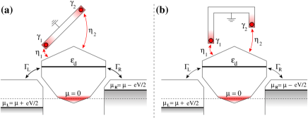
Figure 1: A schematic outline of the mathematical model formulated in Eqs. (1)-(8), assuming $eV<0$. The model may be realized, for example, with a straight TS, as shown in (a), or with an arched TS, as shown in (b).

The Hamiltonian of the TS is

$$\hat{H}_{\text{TS}}=\frac{i}{2}\xi\gamma_{2}\gamma_{1},$$ (2)

where the Majorana operators satisfy $\gamma_{k}^{\dagger}=\gamma_{k}$, $\{\gamma_{k},\gamma_{j}\}=2\delta_{kj}$, $k,j=1,2$ and a finite overlap of the MBSs is taken into account by finite values of the energy $\xi$. The interaction between the QD and TS is described by the following tunneling Hamiltonian

$$\hat{H}_{\text{QD-TS}}=\eta_{1}^{*}d^{\dagger}\gamma_{1}+\eta_{2}^{*}d^{\dagger}\gamma_{2}+\text{H.c.}$$ (3)

Here the tunneling matrix elements have the form

$$\eta_{k}=|\eta_{k}|e^{i\phi_{k}},\quad k=1,2.$$ (4)

The amplitude $|\eta_{k}|$ describes the strength of the tunneling coupling between the QD and Majorana mode $\gamma_{k}$, $k=1,2$. Below we will assume a specific preparation of the system with $|\eta_{1}|\gg|\eta_{2}|$. This corresponds to a relatively simpler technological preparation of the QD located at unequal distances to the ends of the TS as, for example, in Ref. Deng et al. (2018). Specifically, the QD is located closer to the Majorana mode $\gamma_{1}$. Implementations with $|\eta_{1}|\gtrsim|\eta_{2}|$, that is with a more symmetric location of the QD with respect to the ends of the TS, would require an advanced technology, for example, preparing a TS with a more complex shape Liu and Baranger (2011). The Majorana tunneling phases $\phi_{k}$, $k=1,2$, are of particular importance. The tunneling phase difference $\Delta\phi=\phi_{1}-\phi_{2}$ gives rise to Majorana interference in the system. Various physical observables acquire a dependence on $\Delta\phi$. In particular, fluctuation fingerprints of the Majorana interference in the finite frequency quantum noise are encoded in its dependence on the Majorana phase difference $\Delta\phi$.

The electric currents, in particular their fluctuations, are measured in two normal metallic contacts coupled via tunneling to the QD. The two contacts are denoted as left ($L$) and right ($R$). Their Hamiltonian is

$$\hat{H}_{\text{C}}=\sum_{l=L,R}\sum_{k}\epsilon_{k}c_{lk}^{\dagger}c_{lk},$$ (5)

In Eq. (5) it is assumed that both contacts have the same continuum energy spectrum $\epsilon_{k}$. It gives rise to a certain density of states $\nu(\epsilon)$ which is a function of energy. The continuum energy spectrum of the contacts is involved in various physical observables only through the density of states whose energy dependence is often neglected, $\nu(\epsilon)\approx\nu_{C}/2$. This assumes a weak energy dependence of $\nu(\epsilon)$ in the energy domain where quantum transport is most effective Altland and Simons (2010). The contacts are in their equilibrium states which are characterized by the corresponding Fermi-Dirac distributions,

$$n_{L,R}(\epsilon)=\frac{1}{\exp\bigl{(}\frac{\epsilon-\mu_{L,R}}{k_{\text{B}}T}\bigr{)}+1}.$$ (6)

In Eq. (6) we assume that the contacts have the same temperature $T$ but their chemical potentials,

$$\mu_{L,R}=\mu\pm eV/2,$$ (7)

are different for finite bias voltages $V$. Below, in Section IV, we perform numerical calculations assuming that the bias voltage is chosen such that $eV<0$.

The tunneling Hamiltonian taking into account the coupling between the contacts and QD has the form

$$\hat{H}_{\text{QD-C}}=\sum_{l=L,R}\mathcal{T}_{l}\sum_{k}c_{lk}^{\dagger}d+\text{H.c.},$$ (8)

assuming independence of the tunneling matrix elements of the quantum numbers $k$ characterizing the states of the contacts. The matrix elements $\mathcal{T}_{L,R}$ together with the density of states $\nu_{C}$ of the contacts determine the strengths $\Gamma_{L,R}=\pi\nu_{C}|\mathcal{T}_{L,R}|^{2}$ of the tunneling interactions between the QD and, respectively, the left and right contacts. Below we focus on the situation when $\Gamma_{L}=\Gamma_{R}$. The total tunneling strength is $\Gamma\equiv\Gamma_{L}+\Gamma_{R}$.

The system described by Eqs. (1)-(8) is schematically illustrated in Fig. 1. It may be implemented using various technological structures. For example, the straight TS in Fig. 1(a) corresponds to the structure proposed in Ref. Deng et al. (2018) while the arched TS in Fig. 1(b) corresponds to the structure proposed in Ref. Flensberg (2011) and used, e.g., in Refs. Liu and Baranger (2011); Ricco et al. (2018).

III Quantum noise from the Keldysh field integral

When $V\neq 0$, the system is brought into a nonequilibrium state which has to be dealt with by a proper theoretical tool. Here we use the Keldysh technique implemented within the formalism of the Keldysh field integral Altland and Simons (2010) defined on the Keldysh closed time contour $C_{\text{K}}$ with forward and backward branches labeled, respectively, with $q=\pm$. The general strategy of this formalism assumes a proper formulation of a fermionic problem in terms of coherent states and their eigenvalues which are the Grassmann fields $\chi(t)$, $t\in C_{\text{K}}$, corresponding to the annihilation and creation operators used to express the Hamiltonian of this problem.

Our problem is described by the Hamiltonian

$$\hat{H}=\hat{H}_{\text{QD}}+\hat{H}_{\text{TS}}+\hat{H}_{\text{QD-TS}}+\hat{H}_{C}+\hat{H}_{\text{QD-C}}.$$ (9)

In accordance with the general strategy of the Keldysh field integral, we introduce the Grassmann fields $(\psi(t),\bar{\psi}(t))$, $(\phi_{lk}(t),\bar{\phi}_{lk}(t))$ and $(\zeta(t),\bar{\zeta}(t))$ instead of the operators $(d,d^{\dagger})$, $(c_{lk},c_{lk}^{\dagger})$ and $(\gamma_{1},\gamma_{2})$. Here the bars over the Grassmann fields denote the Grassmann conjugation (G.c.). Various physical observables of interest may be expressed via these Grassmann fields. In particular, the matrix element of the electric current operator between proper coherent states is

$$I_{lq}(t)=\frac{ie}{\hbar}\sum_{k}\bigl{[}\mathcal{T}_{l}\bar{\phi}_{lkq}(t)\psi_{q}(t)-\text{G.c.}\bigr{]},$$ (10)

where $l=L,R$ specifies the contact, $q=\pm$ the branch of $C_{\text{K}}$ and $t$ real time.

The electric current and other physical quantities may be obtained from the Keldysh generating functional which is a field integral over the fields defined on $C_{\text{K}}$

$$[\bar{\Phi}(t),\Phi(t)]\equiv[\bar{\psi}(t),\psi(t);\bar{\phi}_{lk}(t),\phi_{lk}(t);\bar{\zeta}(t),\zeta(t)]$$ (11)

with the integrand specified by the Keldysh action $S_{\text{K}}$,

$$Z[J_{lq}(t)]=\int\mathcal{D}[\bar{\Phi}(t),\Phi(t)]e^{\frac{i}{\hbar}S_{\text{K}}[J_{lq}(t)]},$$ (12)

where the Keldysh action is the sum of the actions of the QD, TS, contacts, tunneling actions and a source action to generate physical quantities of interest,

$$\begin{split}&S_{\text{K}}[J_{lq}(t)]=S_{\text{QD}}[\bar{\psi}_{q}(t),\psi_{q}(t)]\\ &+S_{\text{TS}}[\bar{\zeta}_{q}(t),\zeta_{q}(t)]+S_{\text{C}}[\bar{\phi}_{lkq}(t),\phi_{lkq}(t)]\\ &+S_{\text{QD-TS}}[\bar{\psi}_{q}(t),\bar{\zeta}_{q}(t);\psi_{q}(t),\zeta_{q}(t)]\\ &+S_{\text{QD-C}}[\bar{\psi}_{q}(t),\bar{\phi}_{lkq}(t);\psi_{q}(t),\phi_{lkq}(t)]\\ &+S_{\text{SRC}}[J_{lq}(t)].\end{split}$$ (13)

In Eq. (13) the actions $S_{\text{QD}}$, $S_{\text{TS}}$ and $S_{\text{C}}$ are represented by standard $2\times 2$ matrices in the retarded-advanced space (see Ref. Altland and Simons (2010)). The form of the tunneling actions is obtained from the Hamiltonians in Eqs. (3) and (8):

$$\begin{split}&S_{\text{QD-TS}}[\bar{\psi}_{q}(t),\bar{\zeta}_{q}(t);\psi_{q}(t),\zeta_{q}(t)]=\\ &-\int_{-\infty}^{\infty}dt\{\eta_{1}^{*}[\bar{\psi}_{+}(t)\zeta_{+}(t)+\bar{\psi}_{+}(t)\bar{\zeta}_{+}(t)\\ &-\bar{\psi}_{-}(t)\zeta_{-}(t)-\bar{\psi}_{-}(t)\bar{\zeta}_{-}(t)]+i\eta_{2}^{*}[\bar{\psi}_{+}(t)\zeta_{+}(t)\\ &+\bar{\psi}_{-}(t)\bar{\zeta}_{-}(t)-\bar{\psi}_{-}(t)\zeta_{-}(t)-\bar{\psi}_{+}(t)\bar{\zeta}_{+}(t)]+\text{G.c.}\}\end{split}$$ (14)

$$\begin{split}&S_{\text{QD-C}}[\bar{\psi}_{q}(t),\bar{\phi}_{lkq}(t);\psi_{q}(t),\phi_{lkq}(t)]=\\ &-\int_{-\infty}^{\infty}dt\sum_{l=L,R}\sum_{k}\{\mathcal{T}_{l}[\bar{\phi}_{lk+}(t)\psi_{+}(t)\\ &-\bar{\phi}_{lk-}(t)\psi_{-}(t)]+\text{G.c.}\}.\end{split}$$ (15)

To explore the electric current the source action is chosen as follows:

$$S_{\text{SRC}}[J_{lq}(t)]=-\int_{-\infty}^{\infty}dt\sum_{l=L,R}\sum_{q=\pm}J_{lq}(t)I_{lq}(t).$$ (16)

From the Keldysh generating functional one obtains the average electric current and current-current correlations by differentiations of $Z[J_{lq}(t)]$ over the source field $J_{lq}(t)$:

$$\langle I_{lq}(t)\rangle_{0}=i\hbar\frac{\delta Z[J_{lq}(t)]}{\delta J_{lq}(t)}\biggl{|}_{J_{lq}(t)=0}$$ (17)

$$\langle I_{lq}(t)I_{l^{\prime}q^{\prime}}(t^{\prime})\rangle_{0}=(i\hbar)^{2}\frac{\delta^{2}Z[J_{lq}(t)]}{\delta J_{lq}(t)\delta J_{l^{\prime}q^{\prime}}(t^{\prime})}\biggl{|}_{J_{lq}(t)=0}.$$ (18)

In Eqs. (17) and (18) averaging,

$$\begin{split}&\langle\mathcal{F}[\bar{\Phi}(t_{j}),\Phi(t_{j^{\prime}})]\rangle_{0}\equiv\\ &\int\mathcal{D}[\bar{\Phi}(t),\Phi(t)]e^{\frac{i}{\hbar}S_{\text{K}}^{(0)}}\mathcal{F}[\bar{\Phi}(t_{j}),\Phi(t_{j^{\prime}})]\end{split}$$ (19)

is performed using the Keldysh action without the sources, $S_{\text{K}}^{(0)}\equiv S_{\text{K}}[J_{lq}(t)=0]$.

For measurements of the electric current and its fluctuations in the left contact we put below $l=L$. The mean electric current $I(V,\Delta\phi)$ as a function of the bias voltage $V$ and the Majorana tunneling phase difference $\Delta\phi$ is obtained from Eq. (17) with $l=L$, that is $I(V,\Delta\phi)=\langle I_{Lq}(t)\rangle_{0}$, where $q$ is arbitrary since the average $\langle\cdots\rangle_{0}$ defined in Eq. (19) removes any dependence on $q$. We are interested in the quantum noise which is defined as the greater current-current correlator,

$$\begin{split}&S^{>}(t,t^{\prime};V,\Delta\phi)\equiv\langle\delta I_{L-}(t)\delta I_{L+}(t^{\prime})\rangle_{0},\\ &\delta I_{Lq}(t)\equiv I_{Lq}(t)-I(V,\Delta\phi).\end{split}$$ (20)

Since we deal with stationary nonequilibrium states, the quantum noise depends on $t$ and $t^{\prime}$ only through their difference, $S^{>}(t,t^{\prime};V,\Delta\phi)=S^{>}(t-t^{\prime};V,\Delta\phi)$. The Fourier transform

$$S^{>}(\omega,V,\Delta\phi)=\int_{-\infty}^{\infty}dte^{i\omega t}S^{>}(t;V,\Delta\phi)$$ (21)

provides the finite frequency quantum noise which, depending on the sign of the frequency $\omega$, probes the photon absorption/emission spectra:

$$S^{\text{ab}/\text{em}}(\omega,V,\Delta\phi)=\begin{cases}S^{>}(\omega,V,\Delta\phi),&\quad\omega>0\\ S^{>}(\omega,V,\Delta\phi),&\quad\omega<0.\end{cases}$$ (22)

In our numerical calculations we have only focused on positive frequencies which admit interpretations of the numerical results in terms of photon absorption processes (see Section IV for details).

To examine universal fingerprints of the fluctuation behavior induced by the interference of the MBSs we numerically calculate the differential quantum noise, $\partial S^{>}(\omega,V,\Delta\phi)/\partial V$, which is an experimentally accessible physical quantity Basset et al. (2012). In the numerical calculations we first obtain the finite frequency quantum noise $S^{>}(\omega,V,\Delta\phi)$ from numerical integrations with high precision. Afterwards, using finite differences, we numerically calculate the derivatives $\partial S^{>}(\omega,V,\Delta\phi)/\partial V$ at finite frequencies $\omega$ in a wide rage. Of particular interest is the universal Majorana regime arising when the energy scale characterizing the strength of the tunneling between the QD and TS essentially exceeds the other energy scales of the problem. It may be achieved, for example, if the parameters satisfy the following inequality

$$|\eta_{1}|>\text{max}\{|\epsilon_{d}|,k_{\text{B}}T,|\eta_{2}|,\xi,\Gamma,|eV|\},$$ (23)

which has been assumed in performing our numerical analysis of the finite frequency differential quantum noise discussed in the next section. To interpret the behavior of the differential quantum noise at finite frequencies in terms of emission and absorption processes it may be helpful to recall (see Ref. Smirnov (2019a)) that in the parameter regime specified by Eq. (23) the MBSs induce in the QD a quasiparticle zero-energy state as well as quasiparticle states with the energies $\mp 2|\eta_{1}|$. Due to the coupling of the QD to the contacts the width of the zero-energy state is equal to $\Gamma$ whereas the widths of the states with the energies $\mp 2|\eta_{1}|$ are both equal to $\Gamma/2$. The behavior of the differential quantum noise discussed below is mainly governed by the zero-energy quasiparticle state. Transport processes with initial and final states in the contacts or TS may excite the QD. In the next section under weak excitations of the QD we understand those excitations which are localized within the energy range of order $\Gamma$ around the zero-energy state. Although, as discussed in the next section, large excitations to the states with the energies $\mp 2|\eta_{1}|$ also occur, they are not in the focus of the present work.

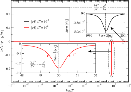
Figure 2: Differential quantum noise $\partial S^{>}(\omega,V)/\partial V$ as a function of the frequency $\omega$ in the absence of direct tunneling between the QD and the second Majorana mode $\gamma_{2}$, that is $|\eta_{2}|=0$. The black curve corresponds to a low bias voltage, $V=V_{1}$, whereas the red curve corresponds to a high bias voltage, $V=V_{2}$, with the specific values $|eV_{1}|/\Gamma=10^{-4}$ and $|eV_{2}|/\Gamma=10^{2}$. Here $\epsilon_{d}/\Gamma=10$, $k_{B}T/\Gamma=10^{-12}$, $|\eta_{1}|/\Gamma=10^{3}$, $\xi/\Gamma=10^{-14}$.

IV Numerical results for the differential quantum noise at finite frequencies

We start our numerical analysis with the situation when Majorana interference is absent, that is, when there is no any dependence on the Majorana tunneling phase difference $\Delta\phi$. This happens for $|\eta_{2}|=0$. In this case, as can be seen in Fig. 2, at low bias voltages, $|eV|\ll\Gamma$, the differential quantum noise as a function of the frequency $\omega$ has a step-like shape (the black curve) with the jump located at $\hbar\omega=|eV|$. At frequencies $\hbar\omega<|eV|$ the differential quantum noise does not depend on $\omega$ forming a plateau with the universal unitary value $e^{3}/4h$ known for the static limit, $\omega\rightarrow 0$ (see, e.g., Refs. Liu et al. (2015a) and Smirnov (2017)). At frequencies $\hbar\omega>|eV|$ the differential quantum noise is strongly suppressed except for a vicinity of the frequency $\hbar\omega=2|\eta_{1}|$. Since at positive frequencies the quantum noise may be interpreted in terms of photon absorption processes (see Section III, Eq. (22), and also Refs. Bathellier et al. (2019); Smirnov (2019a)), such a behavior at low bias voltages indicates that for a given value $V$ of the bias voltage, $|eV|\ll\Gamma$, photon absorption becomes impossible for $\hbar\omega>|eV|$ except for a vicinity of $\hbar\omega=2|\eta_{1}|$ where a photon absorption

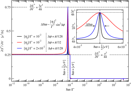
Figure 3: Differential quantum noise $\partial S^{>}(\omega,V,\Delta\phi)/\partial V$ as a function of the frequency $\omega$ at low bias voltages, $|eV|\ll\Gamma$, and in the presence of direct tunneling between the QD and the second Majorana mode $\gamma_{2}$. For all the curves $|eV|/\Gamma=10^{-4}$. The black curve: $|\eta_{2}|/\Gamma=10^{-2}$, $\Delta\phi=\pi/128$. The red curve: $|\eta_{2}|/\Gamma=10^{-2}$, $\Delta\phi=\pi/32$. The blue curve: $|\eta_{2}|/\Gamma=2\times 10^{-2}$, $\Delta\phi=\pi/128$. The other parameters are the same as in Fig. 2.

becomes possible due to transport processes occurring along with the excitation of the QD by energy $\Delta\epsilon=2|\eta_{1}|$ (see Ref. Smirnov (2019a)). The upper inset shows a shallow antiresonance corresponding to such photon absorption. It is located around $\hbar\omega=2|\eta_{1}|$ and the full width of this antiresonance at half of its minimum is equal to $\Gamma/2$. It is interesting to note that at low bias voltages, $|eV|\ll\Gamma$, photon absorption admitted by tunneling of quasiparticles from the left contact to the TS does not contribute to the differential quantum noise $\partial S^{>}(\omega,V)/\partial V$. Indeed, when accompanied by weak excitations of the QD, such tunneling processes would increase the quasiparticle energy by $\Delta\epsilon_{qp}=|eV|/2$ and thus in a vicinity of the frequency $\hbar\omega=|eV|/2$ one could expect that $\partial S^{>}(\omega,V)/\partial V$ has a specific resonance or antiresonance. This is, however, not the case as demonstrated by the black curve. On the other side, the situation at high bias voltages is qualitatively different. As demonstrated by the red curve, the differential quantum noise $\partial S^{>}(\omega,V)/\partial V$ is suppressed by high bias voltages, $|eV|\gg\Gamma$, at all frequencies except for a vicinity of $\hbar\omega=|eV|/2$. Around this frequency there develops an antiresonance in $\partial S^{>}(\omega,V)/\partial V$. As shown in the lower inset, the minimum of this antiresonance is located at $\hbar\omega=|eV|/2$ where the differential quantum noise reaches the universal unitary value $-e^{3}/4h$. The full width $\Delta\hbar\omega$ of the antiresonance at half of its minimum is equal to $\Gamma$,

$$\begin{split}&\frac{\partial S^{>}(\omega,V)}{\partial V}\biggl{|}_{\hbar\omega=|eV|/2}=-\frac{e^{3}}{4h},\\ &\Delta\hbar\omega=\Gamma.\end{split}$$ (24)

Such a frequency dependence of $\partial S^{>}(\omega,V)/\partial V$ reveals that at large bias voltages, $|eV|\gg\Gamma$, the most efficient opening of a photon-absorption channel occurs in a neighborhood of $\hbar\omega=|eV|/2$ where it is admitted by quasiparticle tunneling from the left contact to the TS. These tunneling processes occur together with weak excitations of the QD in such a way that in the final state the quasiparticle energy is increased by $\Delta\epsilon_{qp}=|eV|/2$ and the QD energy is increased or decreased by $\Delta\epsilon\lesssim\Gamma$ in accordance with the location of the minimum and the characteristic width of the observed antiresonance.

When $|\eta_{2}|$ is finite, it provides a direct tunneling mechanism between the QD and the second Majorana mode $\gamma_{2}$. Now the first and second Majorana modes, $\gamma_{1}$ and $\gamma_{2}$, meet at the QD where they may interfere. This interference is controlled by the difference of the Majorana tunneling phases $\Delta\phi=\phi_{1}-\phi_{2}$ which essentially determines the differential quantum noise and brings fundamental changes in its frequency dependence. As one can see in Fig. 3, in contrast to the case with $|\eta_{2}|=0$ and $|eV|\ll\Gamma$, here for all the three curves, in addition to the already known step-like shape, one observes a resonance in $\partial S^{>}(\omega,V,\Delta\phi)/\partial V$ in a vicinity of the frequency $\hbar\omega=|eV|/2$. As in Fig. 2, on the plateau of the step $\partial S^{>}(\omega,V,\Delta\phi)/\partial V=e^{3}/4h$ whereas the maximum of the resonance arising on top of this plateau reaches another universal unitary value,

$$\frac{\partial S^{>}(\omega,V,\Delta\phi)}{\partial V}\biggl{|}_{\hbar\omega=|eV|/2}=\frac{3e^{3}}{4h},$$ (25)

The inset shows in more detail the shape of the resonance in each of the three curves, particularly, the variation of its full width $\Delta\hbar\omega$ at half of its maximum. It is clearly seen that $\Delta\hbar\omega$ strongly depends on both $|\eta_{2}|$ and $\Delta\phi$. Our numerical calculations reveal that

$$\Delta\hbar\omega\sim\frac{(|\eta_{2}|\sin\Delta\phi)^{2}}{\Gamma}.$$ (26)

In accordance with Fig. 2, the resonance disappears for $|\eta_{2}|=0$. Moreover, it also disappears when $\Delta\phi=0,\pi$. The strong dependence of this resonance on the Majorana phase difference $\Delta\phi$ is suggestive of its pure Majorana interference nature. It also may be interpreted as a bound state in the continuum related to the zero-energy peak in the spectral function of the TS (see, e.g., Ref. Ramos-Andrade et al. (2019)). The Majorana interference projects this zero-energy peak in the spectral function onto the above resonance of finite width $\Delta\hbar\omega$ in the differential quantum noise and in this way turns it into a quasi-BIC. This BIC may also be revealed by means of interference effects captured by the conductance but that would require a more complicated system with at least two TSs where the BIC manifests as a zero-bias antiresonance in the conductance as has been shown in Ref. Ramos-Andrade et al. (2019). In contrast, the differential quantum noise at finite frequencies enables one to detect this BIC in a simpler system using only one TS. Here at low bias voltages, $|eV|\ll\Gamma$, photon absorption processes admitted by weak excitations of the QD and the quasiparticle tunneling from the left contact to the TS are activated by the Majorana interference and reveal the BIC in a vicinity of the frequency $\hbar\omega=|eV|/2$ as the above discussed resonance with the universal unitary maximum $3e^{3}/4h$. More importantly, since Majorana fluctuation fingerprints are more unique than those of Majorana mean currents, the differential quantum noise at finite frequencies provides a reliable tool to identify BICs as originating from Majorana states and not from other states having non-Majorana nature. In particular, as will be shown below (see Fig. 8 and the corresponding discussion), the differential quantum noise does not exhibit any resonance at the frequency $\hbar\omega=|eV|/2$ when the MBSs are replaced with Andreev bound states (ABSs) coupled to the QD. Thus, the resonance in

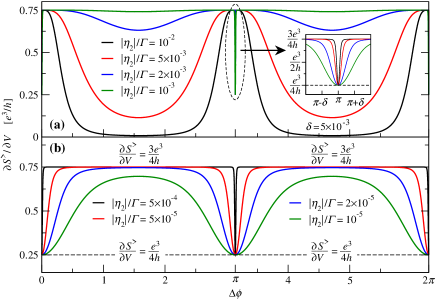
Figure 4: Differential quantum noise $\partial S^{>}(\omega,V,\Delta\phi)/\partial V$ as a function of the Majorana phase difference $\Delta\phi$ at $\hbar\omega=|eV|/2$, $|eV|/\Gamma=10^{-4}$. Panel (a): $|\eta_{2}|/\Gamma=10^{-2}$ (black curve), $|\eta_{2}|/\Gamma=5\times 10^{-3}$ (red curve), $|\eta_{2}|/\Gamma=2\times 10^{-3}$ (blue curve), $|\eta_{2}|/\Gamma=10^{-3}$ (green curve). Panel (b): $|\eta_{2}|/\Gamma=5\times 10^{-4}$ (black curve), $|\eta_{2}|/\Gamma=5\times 10^{-5}$ (red curve), $|\eta_{2}|/\Gamma=2\times 10^{-5}$ (blue curve), $|\eta_{2}|/\Gamma=10^{-5}$ (green curve). The other parameters are the same as in Fig. 2.

$\partial S^{>}(\omega,V,\Delta\phi)/\partial V$ characterized by the universal unitary maximum $3e^{3}/4h$ at the frequency $\hbar\omega=|eV|/2$ is a unique signature that the BIC has the Majorana origin and does not result from other quantum states. On the other side, since mean currents might be controversial with respect to Majorana states, the non-Majorana nature of the BIC could have still been assumed if one had restricted the analysis of the BIC only by the differential conductance measurements Ramos-Andrade et al. (2019) which are still important and should be performed as the first step before probing the BIC via more involved measurements such as, for example, measurements of the differential quantum noise at finite frequencies. We emphasize that the the Majorana interference plays here a fundamental role activating the photon-absorption channel around $\hbar\omega=|eV|/2$ for low bias voltages $|eV|\ll\Gamma$. Indeed, as we have already seen in Fig. 2, although opening of this photon-absorption channel is also admitted for $|\eta_{2}|=0$, without the Majorana interference this channel is not active in the sense that it does not produce any additional finite contribution to the differential quantum noise $\partial S^{>}(\omega,V,\Delta\phi)/\partial V$.

To see how the universal resonance develops and disappears at low bias voltages, $|eV|\ll\Gamma$, we analyze the value of the differential quantum noise at $\hbar\omega=|eV|/2$ as a function of $\Delta\phi$ for various values of $|\eta_{2}|$. From the previous discussion we know that, on one side, this resonance must disappear for $\Delta\phi\rightarrow 0,\pi$ or $|\eta_{2}|\rightarrow 0$ and that, on the other side, its universal unitary maximum $3e^{3}/4h$ is already reached for very small values of the Majorana phase difference, such as $\Delta\phi=\pi/128$, when $|\eta_{2}|$ is finite. Thus one could naturally conclude that for a finite value of $|\eta_{2}|$ the resonance arises as a jump for arbitrarily small deviations of $\Delta\phi$ from $0$ and $\pi$. However, our numerical results shown in Fig. 4 demonstrate that this is not so and the behavior of the resonance is highly nontrivial. As one can see in Fig. 4(a) showing results for larger values of $|\eta_{2}|$, the differential quantum noise at $\hbar\omega=|eV|/2$ indeed quickly grows from the universal unitary plateau $e^{3}/4h$ at $\Delta\phi=0,\pi$ to the universal unitary maximum $3e^{3}/4h$. However, if $|\eta_{2}|$ is very large, $\partial S^{>}(\omega,V,\Delta\phi)/\partial V$ is strongly suppressed far from $\Delta\phi=0,\pi$ as demonstrated in Fig. 4(a) by the black curve corresponding to the value of $|\eta_{2}|$ which has also been used to obtain the black and red curves in Fig. 3. Thus for large values of $|\eta_{2}|$ the resonance is fully developed in small regions centered around the points $\Delta\phi=0,\pi$ in whose extremely narrow vicinities (located fully within these small regions) the resonance disappears recovering the universal unitary plateau $e^{3}/4h$. The inset in Fig. 4(a) shows one of these extremely narrow vicinities, namely, the one with $\Delta\phi=\pi$. Clearly, these extremely narrow vicinities should expand when $|\eta_{2}|$ decreases and this is what one observes in the inset. Upon decreasing $|\eta_{2}|$ such expanding should eventually decrease the differential quantum noise in the small regions, where $\partial S^{>}(\omega,V,\Delta\phi)/\partial V=3e^{3}/4h$, and increase $\partial S^{>}(\omega,V,\Delta\phi)/\partial V$ in the wide regions, where it is strongly suppressed, making it equal to the universal unitary plateau $e^{3}/4h$ in the whole range of $\Delta\phi$ for sufficiently small values of $|\eta_{2}|$. However, before this situation is achieved, one observes that when $|\eta_{2}|$ decreases, the resonance is fully developed in wider and wider regions of the Majorana phase difference as it is demonstrated in Fig. 4(b). Indeed, as one can see, the black and red curves in Fig. 4(b) have wide plateaus on which $\partial S^{>}(\omega,V,\Delta\phi)/\partial V=3e^{3}/4h$. This corresponds to the situation when the resonance fully develops already for very small deviations from $\Delta\phi=0,\pi$ and reaches its universal unitary maximum $3e^{3}/4h$ almost in the whole range of $\Delta\phi$. Note that this behavior happens when $|\eta_{2}|$ is about seven orders of magnitude smaller than $|\eta_{1}|$. This emphasizes that even very weak coupling of the second Majorana mode $\gamma_{2}$ to the QD may fundamentally change the behavior of the differential quantum noise. Only for very small values of $|\eta_{2}|$ the universal unitary plateaus $3e^{3}/4h$ are destroyed and, as can be seen from the blue and green curves in Fig. 4(b), $\partial S^{>}(\omega,V,\Delta\phi)/\partial V$ starts to decrease down to the universal unitary plateau $e^{3}/4h$ for all values of $\Delta\phi$.

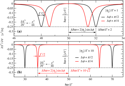
Figure 5: Differential quantum noise $\partial S^{>}(\omega,V,\Delta\phi)/\partial V$ as a function of the frequency $\omega$ at high bias voltages, $|eV|\gg\Gamma$, and in the presence of direct tunneling between the QD and the second Majorana mode $\gamma_{2}$. For all the curves $|eV|/\Gamma=10^{2}$. Panel (a): $|\eta_{2}|/\Gamma=1$ and $\Delta\phi=\pi/2$ (black curve), $\Delta\phi=\pi/4$ (red curve). Panel (b): $|\eta_{2}|/\Gamma=10$ and $\Delta\phi=\pi/2$ (black curve), $\Delta\phi=\pi/4$ (red curve). The other parameters are the same as in Fig. 2.

Majorana quantum noise in strongly nonequilibrium states induced by high bias voltages, $|eV|\gg\Gamma$, is particularly appealing for future experiments. Indeed, in this case $\partial S^{>}(\omega,V,\Delta\phi)/\partial V$ turns out to be extremely sensitive to the Majorana interference especially for $|\eta_{2}|\gtrsim\Gamma$. As has been shown in Fig. 2, for $|\eta_{2}|=0$ and high bias voltages, $|eV|\gg\Gamma$, the differential quantum noise is suppressed for all frequencies except for a vicinity of $\hbar\omega=|eV|/2$. Around this frequency there arises an antiresonance with the universal unitary minimum $-e^{3}/4h$ located at $\hbar\omega=|eV|/2$. The full width of this antiresonance at half of its minimum is equal to $\Gamma$. As demonstrated by Fig. 5, in the presence of direct tunneling between the QD and the second Majorana mode $\gamma_{2}$, that is when $|\eta_{2}|\neq 0$, this antiresonance is split into two antiresonances. From our numerical calculations we find that the minima of these two antiresonances are located symmetrically with respect to the frequency $\hbar\omega=|eV|/2$, that is equidistantly from the location of the minimum of the original antiresonance, specifically, at the two frequencies

$$\hbar\omega_{\pm}=\frac{|eV|}{2}\pm 2|\eta_{2}|\sin\Delta\phi.$$ (27)

At these two frequencies the differential quantum noise reaches the same universal unitary minimum $-e^{3}/4h$ as the one of the original antiresonance. Moreover, the two antiresonances centered around $\hbar\omega_{\pm}$ are twice narrower than the original antiresonance from which they have emerged via the above mentioned splitting. That is they have the same full widths $\Delta\hbar\omega$, equal to $\Gamma/2$, at half of their universal unitary minimum $-e^{3}/4h$,

$$\begin{split}&\frac{\partial S^{>}(\omega,V,\Delta\phi)}{\partial V}\biggl{|}_{\omega=\omega_{\pm}}=-\frac{e^{3}}{4h},\\ &\Delta\hbar\omega=\frac{\Gamma}{2}.\end{split}$$ (28)

Alternatively, instead of the above described picture illustrating the emergence of the above two antiresonances as a split of the original antiresonance one might conceive of a resonance induced by the Majorana interference and interpret it in terms of the BIC discussed in connection with Fig. 3. This resonance develops in the middle of the original antiresonance as soon as $|\eta_{2}|\neq 0$. The height of this resonance

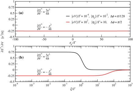
Figure 6: Differential quantum noise $\partial S^{>}(\omega,V,\Delta\phi)/\partial V$ at the resonance and antiresonance frequencies. Panel (a): As a function of the QD energy level $\epsilon_{d}$ at the resonance frequency $\hbar\omega=|eV|/2$ (black curve) and antiresonance frequencies $\omega=\omega_{\pm}$ (red curve). For both curves the overlap energy $\xi/\Gamma=10^{-14}$. Panel (b): As a function of the overlap energy $\xi$ at the resonance frequency $\hbar\omega=|eV|/2$ (black curve) and antiresonance frequencies $\omega=\omega_{\pm}$ (red curve). For both curves the QD energy level $\epsilon_{d}/\Gamma=10$. In both panels for the black curves $|eV|/\Gamma=10^{-4}$, $|\eta_{2}|/\Gamma=10^{-2}$, $\Delta\phi=\pi/128$ whereas for the red curves $|eV|/\Gamma=10^{2}$, $|\eta_{2}|/\Gamma=10$, $\Delta\phi=\pi/2$. The other parameters are the same as in Fig. 2.

approaches the universal unitary value $e^{3}/4h$ when its maximal value approaches zero at $\hbar\omega=|eV|/2$. The bottom of the resonance is reached at the two points $\hbar\omega_{\pm}$ with the distance between them

$$|\hbar\omega_{+}-\hbar\omega_{-}|=4|\eta_{2}||\sin\Delta\phi|.$$ (29)

In experiments one may vary the Majorana phase difference $\Delta\phi$ and observe how the two antiresonances move with respect to each other. Measuring then the maximal distance between the minima of the antiresonances one obtains the maximal value of $|\hbar\omega_{+}-\hbar\omega_{-}|$, that is $4|\eta_{2}|$. After that for any given distance between the minima of the antiresonances, $|\hbar\omega_{+}-\hbar\omega_{-}|$, one may obtain the corresponding Majorana phase difference as $|\sin\Delta\phi|=|\hbar\omega_{+}-\hbar\omega_{-}|/4|\eta_{2}|$. Therefore detecting the two antiresonances, specifically, the locations of their minima at high bias voltages, $|eV|\gg\Gamma$, would enable to determine the frequencies $\hbar\omega_{\pm}$ and, in this way, measure the values of $|\eta_{2}|$ and $\Delta\phi$ in experiments on nonequilibrium finite frequency quantum noise driven by Majorana interference.

Let us now verify the universality of the Majorana resonance and antiresonances at, respectively, low and high bias voltages. The universality assumes independence of the resonance and antiresonances on the gate voltage controlling the position of the QD energy level $\epsilon_{d}$. As one can see in Fig. 6(a), both the resonance and antiresonances remain unchanged when $\epsilon_{d}$ is varied over a wide range. Note, that here we have also included negative values of $\epsilon_{d}$ to confirm our above statement that in the universal Majorana regime, Eq. (23), the differential quantum noise does not depend on $\epsilon_{d}$ both for $\epsilon_{d}>0$ and $\epsilon_{d}<0$.

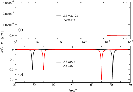
Figure 7: Differential quantum noise $\partial S^{>}(\omega,V,\Delta\phi)/\partial V$ as a function of the frequency $\omega$ for strongly overlapping MBSs characterized by $\xi/\Gamma=2\times 10^{2}$. Panel (a): Low bias voltages, $|eV|\ll\Gamma$, with the specific values of the parameters $|\eta_{2}|/\Gamma=10^{-2}$, $|eV|/\Gamma=10^{-4}$ and $\Delta\phi=\pi/128$ (black curve), $\Delta\phi=\pi/2$ (red curve). Panel (b): High bias voltages, $|eV|\gg\Gamma$, with the specific values of the parameters $|\eta_{2}|/\Gamma=10$, $|eV|/\Gamma=10^{2}$ and $\Delta\phi=\pi/2$ (black curve), $\Delta\phi=\pi/4$ (red curve). The other parameters are the same as in Fig. 2.

It is also important to explore how the differential quantum noise at the resonance and antiresonance frequencies behaves at large values of $\xi$ that is when the overlap of the MBSs is strong as may happen for short distances between the MBSs. In this case the MBSs communicate through the TS and this communication may provide an additional interference channel. Fig. 6(b) demonstrates that when the MBSs start to strongly overlap, the differential quantum noise is significantly suppressed both at the resonance frequency $\hbar\omega=|eV|/2$ for low bias voltages, $|eV|\ll\Gamma$, and at the antiresonance frequencies $\omega_{\pm}$ for high bias voltages, $|eV|\gg\Gamma$. To explore in more detail the fate of the resonance and antiresonances for strongly overlapping MBSs we have analyzed the frequency dependence of the differential quantum noise at large values of $\xi$. In the regime of low bias voltages, $|eV|\ll\Gamma$, shown in Fig. 7(a), we find that the communication between the MBSs through the TS results in a disappearance of the resonance at $\hbar\omega=|eV|/2$ for all values of the Majorana phase difference $\Delta\phi$. Moreover, the dependence on $\Delta\phi$ becomes very weak as demonstrated by the black and red curves which are very close to each other even for the values of $\Delta\phi$ chosen to reach the maximal distance between the curves. Although the step-like behavior (with the jump located at $\hbar\omega=|eV|$) is still present, the differential quantum noise is significantly suppressed below the universal unitary plateau arising at small values of $\xi$, that is $\partial S^{>}(\omega,V,\Delta\phi)/\partial V\ll e^{3}/4h$. A more interesting behavior is observed in the regime of high bias voltages, $|eV|\gg\Gamma$, shown in Fig. 7(b). Here we find two major changes in comparison with the picture discussed above for small values of $\xi$. First, the minima of the two antiresonances become unequal and significantly deviate from the universal unitary minimum $-e^{3}/4h$. Second, the locations of these minima shift from the frequencies $\omega_{\pm}$ (see Eq. (27)) to some other frequencies. For larger values of $\xi$ both the deviations from the universal unitary minimum and the shifts from the frequencies $\omega_{\pm}$ increase even further.

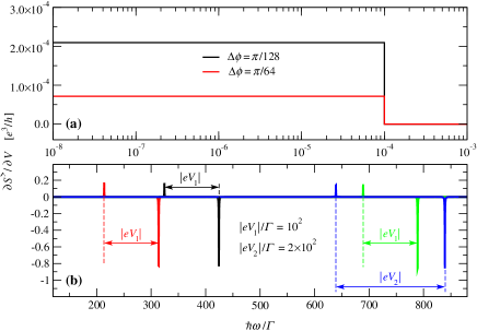
Figure 8: Differential quantum noise $\partial S^{>}(\omega,V,\Delta\phi)/\partial V$ as a function of the frequency $\omega$ for ABSs emerging in our model when the Majorana tunneling amplitudes have the same order, $|\eta_{2}|\sim|\eta_{1}|$, and the overlap energy $\xi$ is large. Specifically, here we use $\xi/\Gamma=8\times 10^{2}$. Panel (a): Low bias voltages, $|eV|\ll\Gamma$, with the specific values of the parameters $|\eta_{2}|/\Gamma=2\times 10^{2}$, $|eV|/\Gamma=10^{-4}$ and $\Delta\phi=\pi/128$ (black curve), $\Delta\phi=\pi/64$ (red curve). Panel (b): High bias voltages, $|eV|\gg\Gamma$. The black curve: $|\eta_{2}|/\Gamma=2\times 10^{2}$, $\Delta\phi=\pi/2$, $|eV|=|eV_{1}|$. The red curve: $|\eta_{2}|/\Gamma=2\times 10^{2}$, $\Delta\phi=\pi/4$, $|eV|=|eV_{1}|$. The green curve: $|\eta_{2}|/\Gamma=4\times 10^{2}$, $\Delta\phi=\pi/2$, $|eV|=|eV_{1}|$. The blue curve: $|\eta_{2}|/\Gamma=4\times 10^{2}$, $\Delta\phi=\pi/2$, $|eV|=|eV_{2}|$. Here $|eV_{1}|/\Gamma=10^{2}$, $|eV_{2}|/\Gamma=2\times 10^{2}$. The other parameters are the same as in Fig. 2.

Finally, we would like to compare the above discussed behavior of the differential quantum noise induced by the MBSs, in particular its resonance and antiresonances brought by the Majorana interference, with the differential quantum noise induced by ABSs. Transport phenomena relevant to ABSs are captured by our theoretical model in a certain range of its parameters. Specifically, when the overlap energy $\xi$ is large and the Majorana tunneling amplitudes are of the same order, $|\eta_{2}|\sim|\eta_{1}|$, our theoretical model describes (see Ref. Deng et al. (2018)) ABSs coupled to the QD. Note, that a different regime which is also specified by the Majorana tunneling amplitudes of the same order, $|\eta_{2}|\sim|\eta_{1}|$, but in which the overlap energy $\xi$ remains small would not be appropriate to model ABSs because it would describe the MBSs in a system with a curved TS corresponding to Fig. 1(b) whose analysis we would like to postpone for a future research. To understand how the differential quantum noise changes when the MBSs are replaced with the ABSs we have performed a numerical analysis for the case of ABSs coupled to the QD. It turns out that, in contrast to the MBSs, the differential quantum noise driven by the ABSs does not have any resonance at the frequency $\hbar\omega=|eV|/2$ in the regime of low bias voltages, $|eV|\ll\Gamma$. Indeed, as demonstrated in Fig. 8(a), the differential quantum noise has the expected step-like behavior (with the jump located at $\hbar\omega=|eV|$) but no any resonance at $\hbar\omega=|eV|/2$ appears for any value of $\Delta\phi$. Moreover, the differential quantum noise is strongly suppressed below the universal unitary plateau $e^{3}/4h$. We find that this suppression cannot be compensated by varying $\Delta\phi$ whose increase suppresses $\partial S^{>}(\omega,V,\Delta\phi)/\partial V$ even further as demonstrated by the red curve. In the regime of high bias voltages, $|eV|\gg\Gamma$, the ABSs have much more interesting fluctuation fingerprints which are essentially different from the ones characterizing the MBSs. Recall that the MBSs give rise to two antiresonances with equal universal unitary minima at which $\partial S^{>}(\omega,V,\Delta\phi)/\partial V=-e^{3}/4h$. The minima are located at the two frequencies $\omega_{\pm}$ (see Fig. 5 and Eq. (27)). The distance between these antiresonances depends on both $|\eta_{2}|$ and $\Delta\phi$. In contrast, as one can see in Fig. 8(b), the ABSs give rise to resonance and antiresonance and not to a pair of antiresonances as it happens for the MBSs. Further, in this resonance-antiresonance pairs induced by the ABSs the amplitudes of the resonance and antiresonance are not equal. Moreover, the frequencies of the ABS resonance and antiresonance are different from the frequencies $\omega_{\pm}$ of the MBS antiresonances. As demonstrated by the black and red curves in Fig. 8(b), the frequencies of the ABS resonance and antiresonance depend on $\Delta\phi$. They also depend on $|\eta_{2}|$ as demonstrated by the black and green curves. However, in contrast to the distance between the MBS antiresonances, the distance between the ABS resonance and antiresonance depends neither on $\Delta\phi$ nor on $|\eta_{2}|$ as one clearly observes from the black, red and green curves. Our numerical analysis reveals that in the ABS range of our model and in the regime specified by Eq. (23) the distance between the ABS resonance and antiresonance depends only on the bias voltage and, in fact, it is equal to $|eV|$ as, in particular, exemplified by the green and blue curves.

V Conclusion

In this work we have numerically investigated universal fluctuation fingerprints of Majorana interference in the differential quantum noise $\partial S^{>}(\omega,V,\Delta\phi)/\partial V$ at finite frequencies $\omega$ in a system where a QD is linked via tunneling to MBSs of a TS with the tunneling phase difference $\Delta\phi$. Nonequilibrium states of this system are induced by a bias voltage $V$. Both low and high bias voltages have been considered. In the regime of low bias voltages it has been found that when the MBSs do not interfere, the differential quantum noise as a function of the frequency has a step-like shape with the universal unitary Majorana plateau $e^{3}/4h$ for $\hbar\omega<|eV|$ and with strong suppression of $\partial S^{>}(\omega,V)/\partial V$ for $\hbar\omega>|eV|$. In presence of the Majorana interference we have discovered that in a vicinity of the frequency $\hbar\omega=|eV|/2$ there develops a narrow resonance whose characteristic width is proportional to $\sin^{2}\Delta\phi$. The maximum of this resonance reaches another universal unitary Majorana value, namely $3e^{3}/4h$, at $\hbar\omega=|eV|/2$. The appearance of this resonance has been explained in terms of an additional photon-absorption channel. This channel is energetically admitted by weak excitations of the QD and tunneling processes from the left contact to the TS. However, opening of this additional photon-absorption channel is activated only by the Majorana interference which gives an additional finite contribution in the form of the above Majorana resonance in $\partial S^{>}(\omega,V,\Delta\phi)/\partial V$. Exploring the regime of high bias voltages we have found that in absence of the Majorana interference the differential quantum noise as a function of the frequency is strongly suppressed everywhere except for a vicinity of the frequency $\hbar\omega=|eV|/2$. Here $\partial S^{>}(\omega,V)/\partial V$ has an antiresonance with the minimum equal to the universal unitary Majorana value $-e^{3}/4h$. This minimum is located at $\hbar\omega=|eV|/2$. The characteristic width of this antiresonance is determined by the strength of the tunneling between the QD and contacts. When the Majorana interference appears, this antiresonance splits into two antiresonances. The minima of these antiresonances are the same as the minimum of the original antiresonance, that is they both reach the universal unitary Majorana value $-e^{3}/4h$. They are located at two finite frequencies $\hbar\omega_{\pm}$ specified by $V$ and $\Delta\phi$. The characteristic widths of the two antiresonances are equal and twice less than the width of the original antiresonance. An alternative interpretation of the two antiresonances has been given in terms of a resonance emerging at the minimum of the original antiresonance. Specifically, for high bias voltages the Majorana interference also activates the additional photon-absorption channel discussed for the case of low bias voltages and gives an additional finite contribution to the differential quantum noise. This finite contribution forms in $\partial S^{>}(\omega,V,\Delta\phi)/\partial V$ a resonance at the minimum of the original antiresonance and, as a result, there appear two antiresonances at the frequencies $\hbar\omega_{\pm}$. It has been suggested that a detection of the frequencies $\hbar\omega_{\pm}$ might be a practical tool to measure the Majorana phase difference $\Delta\phi$ in experiments on nonequilibrium finite frequency quantum noise. In addition, the universality of the Majorana resonance and antiresonances at, respectively, low and high bias voltages has been demonstrated and the case of strongly overlapping MBSs has been analyzed. Finally, the fluctuation fingerprints explored for the MBSs have been compared with those emerging when the MBSs are replaced with ABSs coupled to the QD. It has been shown that the ABSs give rise to fundamental changes in the behavior of the differential quantum noise as compared to the one induced by the MBSs. In particular, for the ABSs one does not observe any resonance at $\hbar\omega=|eV|/2$ in the low bias regime whereas in the high bias regime instead of two antiresonances with equal amplitudes there appear a resonance and antiresonance with different amplitudes. The frequencies of these ABS resonance and antiresonance are different from the frequencies of the two MBS antiresonances. Moreover, in contrast to the distance between the MBS antiresonances, the distance between the ABS resonance and antiresonance does not depend on $|\eta_{2}|$ and $\Delta\phi$ but depends only on the bias voltage. Specifically, our numerical analysis has revealed that this distance is equal to $|eV|$.

In the present work we have focused on numerical calculations of the differential quantum noise at finite frequencies and predicted an appearance of a resonance and antiresonances induced by Majorana interference. The numerical approach has allowed us to achieve the goals formulated in the introduction, Section I, in particular, to reveal universal unitary values characterizing fluctuation fingerprints of interfering MBSs at finite frequencies. Namely, the maximum and minima of, respectively, the Majorana resonance and antiresonances are quantized to some specific fractions of $e^{3}/h$. There appears a natural question: How can one understand these fractions? Within a pure numerical approach it is hard or, perhaps, impossible to answer this question. Thus, as a possible outlook, it would be useful to obtain an analytical solution or develop an appropriate effective model which would be able to explicitly show how the interfering MBSs result in the numerically predicted fractional values of the differential quantum noise at finite frequencies. Another interesting problem is to investigate universal fingerprints of Majorana interference in the finite frequency quantum noise when nonequilibrium states of a system with MBSs have thermoelectric nature. This might be achieved, e.g., by applying to the system both electric and thermal voltages. If the MBSs interfere, one may expect that the differential quantum noise will have a specific universal behavior at finite frequencies. How these frequencies depend on various parameters controlling both the Majorana interference and nonequilibrium in the system is an important problem for fundamental and practical research on MBSs.

References

- Yu. Kitaev (2001) A. Yu. Kitaev, “Unpaired Majorana fermions in quantum wires,” Phys.-Usp. 44, 131 (2001).
- Alicea (2012) J. Alicea, “New directions in the pursuit of Majorana fermions in solid state systems,” Rep. Prog. Phys. 75, 076501 (2012).
- Leijnse and Flensberg (2012) M. Leijnse and K. Flensberg, “Introduction to topological superconductivity and Majorana fermions,” Semicond. Sci. Technol. 27, 124003 (2012).
- Sato and Fujimoto (2016) M. Sato and S. Fujimoto, “Majorana fermions and topology in superconductors,” J. Phys. Soc. Japan 85, 072001 (2016).
- Aguado (2017) R. Aguado, “Majorana quasiparticles in condensed matter,” La Rivista del Nuovo Cimento 40, 523 (2017).
- Lutchyn et al. (2018) R. M. Lutchyn, E. P. A. M. Bakkers, L. P. Kouwenhoven, P. Krogstrup, C. M. Marcus, and Y. Oreg, “Majorana zero modes in superconductor-semiconductor heterostructures,” Nat. Rev. Mater. 3, 52 (2018).
- Yu. Kitaev (2003) A. Yu. Kitaev, “Fault-tolerant quantum computation by anyons,” Ann. Phys. 303, 2 (2003).
- Muralidharan et al. (2023) B. Muralidharan, M. Kumar, and C. Li, “Emerging quantum hybrid systems for non-Abelian-state manipulation,” Front. Nanotechnol. 5, 1219975 (2023).
- Tsintzis et al. (2022) A. Tsintzis, R. S. Souto, and M. Leijnse, “Creating and detecting poor man’s Majorana bound states in interacting quantum dots,” Phys. Rev. B 106, L201404 (2022).
- Dvir et al. (2023) T. Dvir, G. Wang, N. van Loo, C.-X. Liu, G. P. Mazur, A. Bordin, S. L. D. ten Haaf, J.-Y. Wang, D. van Driel, F. Zatelli, X. Li, F. K. Malinowski, S. Gazibegovic, G. Badawy, E. P. A. M. Bakkers, M. Wimmer, and L. P. Kouwenhoven, “Realization of a minimal Kitaev chain in coupled quantum dots,” Nature 614, 445 (2023).
- Tsintzis et al. (2024) A. Tsintzis, R. S. Souto, K. Flensberg, J. Danon, and M. Leijnse, “Majorana qubits and non-Abelian physics in quantum dot-based minimal Kitaev chains,” PRX Quantum 5, 010323 (2024).
- Yu et al. (2021) P. Yu, J. Chen, M. Gomanko, G. Badawy, E. P. A. M. Bakkers, K. Zuo, V. Mourik, and S. M. Frolov, “Non-Majorana states yield nearly quantized conductance in proximatized nanowires,” Nat. Phys. 17, 482 (2021).
- Frolov (2021) S. Frolov, “Quantum computing’s reproducibility crisis: Majorana fermions,” Nature (London) 592, 350 (2021).
- Smirnov (2015) S. Smirnov, “Majorana tunneling entropy,” Phys. Rev. B 92, 195312 (2015).
- Hartman et al. (2018) N. Hartman, C. Olsen, S. Lüscher, M. Samani, S. Fallahi, G. C. Gardner, M. Manfra, and J. Folk, “Direct entropy measurement in a mesoscopic quantum system,” Nat. Phys. 14, 1083 (2018).
- Kleeorin et al. (2019) Y. Kleeorin, H. Thierschmann, H. Buhmann, A. Georges, L. W. Molenkamp, and Y. Meir, “How to measure the entropy of a mesoscopic system via thermoelectric transport,” Nat. Commun. 10, 5801 (2019).
- Sela et al. (2019) E. Sela, Y. Oreg, S. Plugge, N. Hartman, S. Lüscher, and J. Folk, “Detecting the universal fractional entropy of Majorana zero modes,” Phys. Rev. Lett. 123, 147702 (2019).
- Smirnov (2021a) S. Smirnov, “Majorana entropy revival via tunneling phases,” Phys. Rev. B 103, 075440 (2021a).
- Smirnov (2021b) S. Smirnov, “Majorana ensembles with fractional entropy and conductance in nanoscopic systems,” Phys. Rev. B 104, 205406 (2021b).
- Pyurbeeva and Mol (2021) E. Pyurbeeva and J. A. Mol, “A thermodynamic approach to measuring entropy in a few-electron nanodevice,” Entropy 23, 640 (2021).
- Ahari et al. (2021) M. T. Ahari, S. Zhang, J. Zou, and Y. Tserkovnyak, “Biasing topological charge injection in topological matter,” Phys. Rev. B 104, L201401 (2021).
- Child et al. (2022a) T. Child, O. Sheekey, S. Lüscher, S. Fallahi, G. C. Gardner, M. Manfra, and J. Folk, “A robust protocol for entropy measurement in mesoscopic circuits,” Entropy 24, 417 (2022a).
- Han et al. (2022) C. Han, Z. Iftikhar, Y. Kleeorin, A. Anthore, F. Pierre, Y. Meir, A. K. Mitchell, and E. Sela, “Fractional entropy of multichannel Kondo systems from conductance-charge relations,” Phys. Rev. Lett. 128, 146803 (2022).
- Pyurbeeva et al. (2022) E. Pyurbeeva, J. A. Mol, and P. Gehring, “Electronic measurements of entropy in meso- and nanoscale systems,” Chem. Phys. Rev. 3, 041308 (2022).
- Child et al. (2022b) T. Child, O. Sheekey, S. Lüscher, S. Fallahi, G. C. Gardner, M. Manfra, A. Mitchell, E. Sela, Y. Kleeorin, Y. Meir, and J. Folk, “Entropy measurement of a strongly coupled quantum dot,” Phys. Rev. Lett. 129, 227702 (2022b).
- Liu and Baranger (2011) D. E. Liu and H. U. Baranger, “Detecting a Majorana-fermion zero mode using a quantum dot,” Phys. Rev. B 84, 201308(R) (2011).
- Fidkowski et al. (2012) L. Fidkowski, J. Alicea, N. H. Lindner, R. M. Lutchyn, and M. P. A. Fisher, “Universal transport signatures of Majorana fermions in superconductor-Luttinger liquid junctions,” Phys. Rev. B 85, 245121 (2012).
- Prada et al. (2012) E. Prada, P. San-Jose, and R. Aguado, “Transport spectroscopy of nanowire junctions with Majorana fermions,” Phys. Rev. B 86, 180503(R) (2012).
- Pientka et al. (2012) F. Pientka, G. Kells, A. Romito, P. W. Brouwer, and F. von Oppen, “Enhanced zero-bias Majorana peak in the differential tunneling conductance of disordered multisubband quantum-wire/superconductor junctions,” Phys. Rev. Lett. 109, 227006 (2012).
- Lin et al. (2012) C.-H. Lin, J. D. Sau, and S. Das Sarma, “Zero-bias conductance peak in Majorana wires made of semiconductor/superconductor hybrid structures,” Phys. Rev. B 86, 224511 (2012).
- Lee et al. (2013) M. Lee, J. S. Lim, and R. López, “Kondo effect in a quantum dot side-coupled to a topological superconductor,” Phys. Rev. B 87, 241402(R) (2013).
- Kundu and Seradjeh (2013) A. Kundu and B. Seradjeh, “Transport signatures of Floquet Majorana fermions in driven topological superconductors,” Phys. Rev. Lett. 111, 136402 (2013).
- Vernek et al. (2014) E. Vernek, P. H. Penteado, A. C. Seridonio, and J. C. Egues, “Subtle leakage of a Majorana mode into a quantum dot,” Phys. Rev. B 89, 165314 (2014).
- Ilan et al. (2014) R. Ilan, J. H. Bardarson, H.-S. Sim, and J. E. Moore, “Detecting perfect transmission in Josephson junctions on the surface of three dimensional topological insulators,” New J. Phys. 16, 053007 (2014).
- Cheng et al. (2014) M. Cheng, M. Becker, B. Bauer, and R. M. Lutchyn, “Interplay between Kondo and Majorana interactions in quantum dots,” Phys. Rev. X 4, 031051 (2014).
- Leijnse (2014) M. Leijnse, “Thermoelectric signatures of a Majorana bound state coupled to a quantum dot,” New J. Phys. 16, 015029 (2014).
- López et al. (2014) R. López, M. Lee, L. Serra, and J. S. Lim, “Thermoelectrical detection of Majorana states,” Phys. Rev. B 89, 205418 (2014).
- Lobos and Das Sarma (2015) A. M. Lobos and S. Das Sarma, “Tunneling transport in NSN Majorana junctions across the topological quantum phase transition,” New J. Phys. 17, 065010 (2015).
- Peng et al. (2015) Y. Peng, F. Pientka, Y. Vinkler-Aviv, L. I. Glazman, and F. von Oppen, “Robust Majorana conductance peaks for a superconducting lead,” Phys. Rev. Lett. 115, 266804 (2015).
- Khim et al. (2015) H. Khim, R. López, J. S. Lim, and M. Lee, “Thermoelectric effect in the Kondo dot side-coupled to a Majorana mode,” Eur. Phys. J. B 88, 151 (2015).
- Sharma and Tewari (2016) G. Sharma and S. Tewari, “Tunneling conductance for Majorana fermions in spin-orbit coupled semiconductor-superconductor heterostructures using superconducting leads,” Phys. Rev. B 93, 195161 (2016).
- van Heck et al. (2016) B. van Heck, R. M. Lutchyn, and L. I. Glazman, “Conductance of a proximitized nanowire in the Coulomb blockade regime,” Phys. Rev. B 93, 235431 (2016).
- Sarma et al. (2016) S. Das Sarma, A. Nag, and J. D. Sau, “How to infer non-Abelian statistics and topological visibility from tunneling conductance properties of realistic Majorana nanowires,” Phys. Rev. B 94, 035143 (2016).
- Ramos-Andrade et al. (2016) J. P. Ramos-Andrade, O. Ávalos-Ovando, P. A. Orellana, and S. E. Ulloa, “Thermoelectric transport through Majorana bound states and violation of Wiedemann-Franz law,” Phys. Rev. B 94, 155436 (2016).
- Lutchyn and Glazman (2017) R. M. Lutchyn and L. I. Glazman, “Transport through a Majorana island in the strong tunneling regime,” Phys. Rev. Lett. 119, 057002 (2017).
- Weymann and Wójcik (2017) I. Weymann and K. P. Wójcik, “Transport properties of a hybrid Majorana wire-quantum dot system with ferromagnetic contacts,” Phys. Rev. B 95, 155427 (2017).
- V. L. Campo, Jr. et al. (2017) V. L. Campo, Jr., L. S. Ricco, and A. C. Seridonio, “Isolating Majorana fermions with finite Kitaev nanowires and temperature: Universality of the zero-bias conductance,” Phys. Rev. B 96, 045135 (2017).
- Liu et al. (2017) C.-X. Liu, J. D. Sau, T. D. Stanescu, and S. Das Sarma, “Andreev bound states versus Majorana bound states in quantum dot-nanowire-superconductor hybrid structures: Trivial versus topological zero-bias conductance peaks,” Phys. Rev. B 96, 075161 (2017).
- Huang et al. (2017) H. Huang, Q.-F. Liang, D.-X. Yao, and Z. Wang, “Majorana -junction in a disordered spin-orbit coupling nanowire with tilted magnetic field,” Physica C: Superconductivity and its Applications 543, 22 (2017).
- Liu et al. (2018) C.-X. Liu, J. D. Sau, and S. Das Sarma, “Distinguishing topological Majorana bound states from trivial Andreev bound states: Proposed tests through differential tunneling conductance spectroscopy,” Phys. Rev. B 97, 214502 (2018).
- Lai et al. (2019) Y.-H. Lai, J. D. Sau, and S. Das Sarma, “Presence versus absence of end-to-end nonlocal conductance correlations in Majorana nanowires: Majorana bound states versus Andreev bound states,” Phys. Rev. B 100, 045302 (2019).
- Tang and Mao (2020) L.-W. Tang and W.-G. Mao, “Detection of Majorana bound states by sign change of the tunnel magnetoresistance in a quantum dot coupled to ferromagnetic electrodes,” Front. Phys. 8, 147 (2020).
- Zhang and Spånslätt (2020) G. Zhang and C. Spånslätt, “Distinguishing between topological and quasi Majorana zero modes with a dissipative resonant level,” Phys. Rev. B 102, 045111 (2020).
- Smirnov (2020) S. Smirnov, “Dual Majorana universality in thermally induced nonequilibrium,” Phys. Rev. B 101, 125417 (2020).
- Chi et al. (2021) F. Chi, T.-Y. He, and G. Zhou, “Photon-assisted average current through a quantum dot coupled to Majorana bound states,” J. Nanoelectron. Optoelectron. 16, 1325 (2021).
- Wang and Huang (2021) Z.-H. Wang and W.-C. Huang, “Dual negative differential of heat generation in a strongly correlated quantum dot side-coupled to Majorana bound states,” Front. Phys. 9, 727934 (2021).
- He et al. (2021) T.-Y. He, H. Sun, and G. Zhou, “Photon-assisted Seebeck effect in a quantum dot coupled to Majorana zero modes,” Front. Phys. 9, 687438 (2021).
- Galambos et al. (2022) T. H. Galambos, F. Ronetti, B. Hetényi, D. Loss, and J. Klinovaja, “Crossed Andreev reflection in spin-polarized chiral edge states due to the Meissner effect,” Phys. Rev. B 106, 075410 (2022).
- Giuliano et al. (2022) D. Giuliano, A. Nava, R. Egger, P. Sodano, and F. Buccheri, “Multiparticle scattering and breakdown of the Wiedemann-Franz law at a junction of interacting quantum wires,” Phys. Rev. B 105, 035419 (2022).
- Buccheri et al. (2022) F. Buccheri, A. Nava, R. Egger, P. Sodano, and D. Giuliano, “Violation of the Wiedemann-Franz law in the topological Kondo model,” Phys. Rev. B 105, L081403 (2022).
- Majek et al. (2022) P. Majek, K. P. Wójcik, and I. Weymann, “Spin-resolved thermal signatures of Majorana-Kondo interplay in double quantum dots,” Phys. Rev. B 105, 075418 (2022).
- Bondyopadhaya and Roy (2022) N. Bondyopadhaya and D. Roy, “Nonequilibrium electrical, thermal and spin transport in open quantum systems of topological superconductors, semiconductors and metals,” J. Stat. Phys. 187, 11 (2022).
- Zou et al. (2022) W.-K. Zou, Q. Wang, and H.-K. Zhao, “Aharonov-Bohm oscillations in the Majorana fermion modulated charge and heat transports through a double-quantum-dot interferometer,” Phys. Lett. A 443, 128219 (2022).
- Wang and Wang (2023) C. Wang and X.-Q. Wang, “Thermoelectric signature of Majorana zero modes in a T-typed double-quantum-dot structure,” Chin. Phys. B 32, 037304 (2023).
- Zou et al. (2023a) W.-K. Zou, N.-W. Li, and F.-L. Chong, “Charge and spin transports through a normal lead coupled to an s-wave superconductor and Majorana fermions,” Phys. Status Solidi B , 2200472 (2023a).
- Huguet et al. (2023) A. Huguet, K. Wrześniewski, and I. Weymann, “Spin effects on transport and zero-bias anomaly in a hybrid Majorana wire-quantum dot system,” Sci. Rep. 13, 17279 (2023).
- Becerra et al. (2023) V. F. Becerra, M. Trif, and T. Hyart, “Quantized spin pumping in topological ferromagnetic-superconducting nanowires,” Phys. Rev. Lett. 130, 237002 (2023).
- Ziesen et al. (2023) A. Ziesen, A. Altland, R. Egger, and F. Hassler, “Statistical Majorana bound state spectroscopy,” Phys. Rev. Lett. 130, 106001 (2023).
- Jin and Li (2022) J. Jin and X.-Q. Li, “Master equation approach for transport through Majorana zero modes,” New J. Phys. 24, 093009 (2022).
- Zou et al. (2023b) W.-K. Zou, Q. Wang, and H.-K. Zhao, “Dynamic heat and charge transports through double-quantum-dot-interferometer modulated by Majorana bound states and time-oscillating Aharonov-Bohm flux,” J. Phys. Condens. Matter 35, 165303 (2023b).
- Yao et al. (2023) C.-Z. Yao, H.-L. Lai, and W.-M. Zhang, “Quantum transport theory of hybrid superconducting systems,” Phys. Rev. B 108, 195402 (2023).
- Wójcik et al. (2024) K. P. Wójcik, T. Domański, and I. Weymann, “Signatures of Kondo-Majorana interplay in ac response,” Phys. Rev. B 109, 075432 (2024).
- Taranko et al. (2023) R. Taranko, K. Wrześniewski, I. Weymann, and T. Domański, “Transient effects in quantum dots contacted via topological superconductor,” arXiv:2312.04488v1 (2023).
- Mourik et al. (2012) V. Mourik, K. Zuo, S. M. Frolov, S. R. Plissard, E. P. A. M. Bakkers, and L. P. Kouwenhoven, “Signatures of Majorana fermions in hybrid superconductor-semiconductor nanowire devices,” Science 336, 1003 (2012).
- Nadj-Perge et al. (2014) S. Nadj-Perge, I. K. Drozdov, J. Li, H. Chen, S. Jeon, J. Seo, A. H. MacDonald, B. A. Bernevig, and A. Yazdani, “Observation of Majorana fermions in ferromagnetic atomic chains on a superconductor,” Science 346, 602 (2014).
- Wang et al. (2022) Z. Wang, H. Song, D. Pan, Z. Zhang, W. Miao, R. Li, Z. Cao, G. Zhang, L. Liu, L. Wen, R. Zhuo, D. E. Liu, K. He, R. Shang, J. Zhao, and H. Zhang, “Plateau regions for zero-bias peaks within 5% of the quantized conductance value ,” Phys. Rev. Lett. 129, 167702 (2022).
- Liu et al. (2015a) D. E. Liu, M. Cheng, and R. M. Lutchyn, “Probing Majorana physics in quantum-dot shot-noise experiments,” Phys. Rev. B 91, 081405(R) (2015a).
- Liu et al. (2015b) D. E. Liu, A. Levchenko, and R. M. Lutchyn, “Majorana zero modes choose Euler numbers as revealed by full counting statistics,” Phys. Rev. B 92, 205422 (2015b).
- Haim et al. (2015) A. Haim, E. Berg, F. von Oppen, and Y. Oreg, “Current correlations in a Majorana beam splitter,” Phys. Rev. B 92, 245112 (2015).
- Valentini et al. (2016) S. Valentini, M. Governale, R. Fazio, and F. Taddei, “Finite-frequency noise in a topological superconducting wire,” Physica E 75, 15 (2016).
- Zazunov et al. (2016) A. Zazunov, R. Egger, and A. Levy Yeyati, “Low-energy theory of transport in Majorana wire junctions,” Phys. Rev. B 94, 014502 (2016).
- Smirnov (2017) S. Smirnov, “Non-equilibrium Majorana fluctuations,” New J. Phys. 19, 063020 (2017).
- Smirnov (2018) S. Smirnov, “Universal Majorana thermoelectric noise,” Phys. Rev. B 97, 165434 (2018).
- Jonckheere et al. (2019) T. Jonckheere, J. Rech, A. Zazunov, R. Egger, A. Levy Yeyati, and T. Martin, “Giant shot noise from Majorana zero modes in topological trijunctions,” Phys. Rev. Lett. 122, 097003 (2019).
- Manousakis et al. (2020) J. Manousakis, C. Wille, A. Altland, R. Egger, K. Flensberg, and F. Hassler, “Weak measurement protocols for Majorana bound state identification,” Phys. Rev. Lett. 124, 096801 (2020).
- Feng and Zhang (2022) G.-H. Feng and H.-H. Zhang, “Probing robust Majorana signatures by crossed Andreev reflection with a quantum dot,” Phys. Rev. B 105, 035148 (2022).
- Smirnov (2023) S. Smirnov, “Majorana differential shot noise and its universal thermoelectric crossover,” Phys. Rev. B 107, 155416 (2023).
- Cao et al. (2023) Z. Cao, G. Zhang, H. Zhang, Y.-X. Liang, W.-X. He, K. He, and D. E. Liu, “Differential current noise as an identifier of Andreev bound states that induce nearly quantized conductance plateaus,” Phys. Rev. B 108, L121407 (2023).
- Ge et al. (2023) J.-F. Ge, K. M. Bastiaans, D. Chatzopoulos, D. Cho, W. O. Tromp, T. Benschop, J. Niu, G. Gu, and M. P. Allan, “Single-electron charge transfer into putative Majorana and trivial modes in individual vortices,” Nat. Commun. 14, 3341 (2023).
- Bathellier et al. (2019) D. Bathellier, L. Raymond, T. Jonckheere, J. Rech, A. Zazunov, and T. Martin, “Finite frequency noise in a normal metal - topological superconductor junction,” Phys. Rev. B 99, 104502 (2019).
- Smirnov (2019a) S. Smirnov, “Majorana finite-frequency nonequilibrium quantum noise,” Phys. Rev. B 99, 165427 (2019a).
- Smirnov (2019b) S. Smirnov, “Dynamic Majorana resonances and universal symmetry of nonequilibrium thermoelectric quantum noise,” Phys. Rev. B 100, 245410 (2019b).
- Gau et al. (2020a) M. Gau, R. Egger, A. Zazunov, and Y. Gefen, “Towards dark space stabilization and manipulation in driven dissipative Majorana platforms,” Phys. Rev. B 102, 134501 (2020a).
- Gau et al. (2020b) M. Gau, R. Egger, A. Zazunov, and Yuval Gefen, “Driven dissipative Majorana dark spaces,” Phys. Rev. Lett. 125, 147701 (2020b).
- Smirnov (2022) S. Smirnov, “Revealing universal Majorana fractionalization using differential shot noise and conductance in nonequilibrium states controlled by tunneling phases,” Phys. Rev. B 105, 205430 (2022).
- Basset et al. (2012) J. Basset, A. Y. Kasumov, C. P. Moca, G. Zaránd, P. Simon, H. Bouchiat, and R. Deblock, “Measurement of quantum noise in a carbon nanotube quantum dot in the Kondo regime,” Phys. Rev. Lett. 108, 046802 (2012).
- de Picciotto et al. (1997) R. de Picciotto, M. Reznikov, M. Heiblum, V. Umansky, G. Bunin, and D. Mahalu, “Direct observation of a fractional charge,” Nature 389, 162 (1997).
- Saminadayar et al. (1997) L. Saminadayar, D. C. Glattli, Y. Jin, and B. Etienne, “Observation of the fractionally charged Laughlin quasiparticle,” Phys. Rev. Lett. 79, 2526 (1997).
- Ramos-Andrade et al. (2019) J. B. Ramos-Andrade, D. Zambrano, and P. A. Orellana, “Fano-Majorana effect and bound states in the continuum on a crossbar-shaped quantum dot hybrid structure,” Ann. Phys. (Berlin) 531, 1800498 (2019).
- Flensberg (2011) K. Flensberg, “Non-Abelian operations on Majorana fermions via single-charge control,” Phys. Rev. Lett. 106, 090503 (2011).
- Ruiz-Tijerina et al. (2015) D. A. Ruiz-Tijerina, E. Vernek, L. G. G. V. Dias da Silva, and J. C. Egues, “Interaction effects on a Majorana zero mode leaking into a quantum dot,” Phys. Rev. B 91, 115435 (2015).
- Hewson (1997) A. C. Hewson, The Kondo Problem to Heavy Fermions (Cambridge University Press, Cambridge, 1997).
- Smirnov and Grifoni (2011) S. Smirnov and M. Grifoni, “Slave-boson Keldysh field theory for the Kondo effect in quantum dots,” Phys. Rev. B 84, 125303 (2011).
- Niklas et al. (2016) M. Niklas, S. Smirnov, D. Mantelli, M. Margańska, N.-V. Nguyen, W. Wernsdorfer, J.-P. Cleuziou, and M. Grifoni, “Blocking transport resonances via Kondo many-body entanglement in quantum dots,” Nat. Commun. 7, 12442 (2016).
- Deng et al. (2018) M.-T. Deng, S. Vaitiekėnas, E. Prada, P. San-Jose, J. Nygård, P. Krogstrup, R. Aguado, and C. M. Marcus, “Nonlocality of Majorana modes in hybrid nanowires,” Phys. Rev. B 98, 085125 (2018).
- Altland and Simons (2010) A. Altland and B. Simons, Condensed Matter Field Theory, 2nd ed. (Cambridge University Press, Cambridge, 2010).
- Ricco et al. (2018) L. S. Ricco, F. A. Dessotti, I. A. Shelykh, M. S. Figueira, and A. C. Seridonio, “Tuning of heat and charge transport by Majorana fermions,” Sci. Rep. 8, 2790 (2018).