Axial, Planar-Diagonal, Body-Diagonal Fields on the Cubic-Spin Spin Glass in d=3:
A Plethora of Ordered Phases under Finite Fields

Abstract

A nematic phase, previously seen in the $d=3$ classical Heisenberg spin-glass system, occurs in the n-component cubic-spin spin-glass system, between the low-temperature spin-glass phase and the high-temperature disordered phase, for number of spin components $n\geq 3$, in spatial dimension $d=3$, thus constituting a liquid-crystal phase in a dirty (quenched-disordered) magnet. Furthermore, under application of a variety of uniform magnetic fields, a veritable plethora of phases are found. Under uniform magnetic fields, 15 different phases and two spin-glass phase diagram topologies, qualitatively different from the conventional spin-glass phase diagram topology, are seen. The chaotic rescaling behaviors and their Lyapunov exponents are calculated in each of these spin-glass phase diagram topologies. These results are obtained from renormalization-group calculations that are exact on the hierarchical lattice and, equivalently, approximate on the hypercubic spatial lattice. Axial, planar-diagonal, or body-diagonal finite-strength uniform fields are applied to $n=2$ and 3 component cubic-spin spin-glass systems in $d=3$.

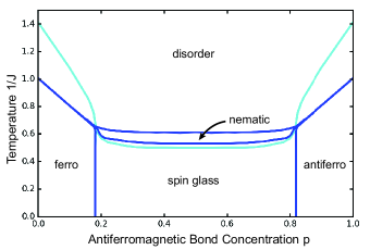
Figure 1: Calculated Artun phase diagrams for the cubic-spin spin-glass systems for zero external field in spatial dimension $d=3$. The phase diagrams are, from top to bottom, for number of components $n=2$ and 3, meaning $n$ Cartesian directions to which the spin aligns or antialigns. A nematic phase appears for $n=3$, between the low-temperature spin-glass phase and the high-temperature disordered phase.

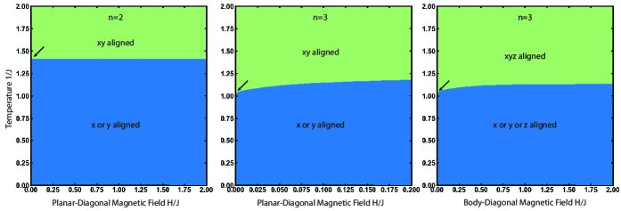
Figure 2: Calculated phase diagrams for the cubic-spin system under planar-diagonal (in the $+xy$ direction) and body-diagonal (in the $+xyz$ direction) magnetic fields, in spatial dimension $d=3$, for $p=0$, namely the ferromagnetic system. In all three cases, a uniaxially aligned symmetry-broken ($x$ or $y$ or $z$ aligned) ordered phase occurs at low temperatures and persists to all high fields. A phase aligned along the applied magnetic field occurs at high temperatures. The phase transition temperatures between these two phases are essentially independent of field strength and join, at the left intercept of the panels, the ferromagnetic transition temperature (marked by arrow) of the zero-field systems. The ordered phases at finite-field are doubly $(n=2)$ or triply $(n=3)$ degenerate. These degeneracies double at ordered phases joined at zero field. The renormalization-group sinks of each phase, to which all points of the phase map under renormalization-group, are given in Table I. These sinks epitomize the ordering of their respective phases.

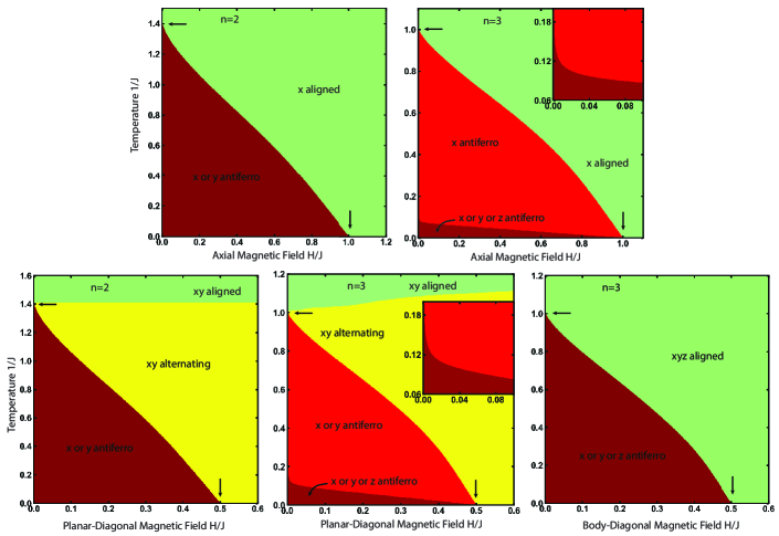
Figure 3: Calculated phase diagrams for the cubic-spin system under external axial (in the $+x$ direction), planar-diagonal (in the $+xy$ direction), body-diagonal (in the $+xyz$ direction) magnetic fields, in spatial dimension $d=3$, for $p=1$, namely the antiferromagnetic system. The top row shows the application of the axial field: At high temperatures or high fields, the system aligns along the applied field. The bottom row shows the application of planar-diagonal or body diagonal magnetic fields: At high temperatures, the system aligns with the applied field. In all panels, at low temperatures and low fields, the system orders in the fully antiferromagnetic phase of the zero-field system. For $n=3$ under axial or planar-diagonal magnetic fields, an intermediate, less degenerate, antiferromagnetic phase occurs in one of the directions of the axial or planar-diagonal field. In these cases, the fully antiferromagnetic phase persists asymptotically close to the zero-field axis, as seen in the insets. For planar-diagonal magnetic field, another ordered phase (doubly degenerate) of $xy$ alternation occurs and continues to all field strengths. All finite-temperature phase boundaries meet at the transition temperature (shown with horizontal arrow) of the zero-field system, which is thus a multiphase point Hoston of three or four phases occurring at finite temperature. The zero-temperature phase transitions (shown with vertical arrow) occur at the ground-state-energy crossings, which also are multiphase points of three phases.

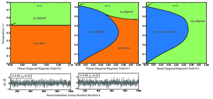
Figure 4: Calculated phase diagrams for the cubic-spin system under planar-diagonal and body-diagonal magnetic fields, in spatial dimension $d=3$, for $p=0.5$, namely the spin-glass system. A spin-glass phase occurs under planar-diagonal magnetic fields. This spin glass phase results from the asymptotic competition, under renormalization-group, of the $+x$ or $+y$ aligned phase and the $xy$ alternating phase. Both of these phases are doubly degenerate, so that the spin-glass phase is quadruply degenerate. Thus, as shown in the second line of the figure, it is $-\beta\mathcal{H}_{ij}(+x,+x)-\beta\mathcal{H}_{ij}(+x,+y)\equiv 2M$ that is chaotic under renormalization-group scale change, whereas in conventional spin-glass phases it is $-\beta\mathcal{H}_{ij}(+x,+x)-\beta\mathcal{H}_{ij}(+x,-x)=2J$ that is chaotic under renormalization-group scale change. In the second line, these calculated chaoses, their calculated Lyapunov exponents $\lambda$ and their runaway exponents $y_{R}$ are given. For $n=2$, the transition temperature is unaffected by field strength. Each of these two spin-glass phase diagram topologies here very different from conventional spin-glass phase diagram topologies: The axis orthogonal to temperature is not a quenched probability but the magnetic field; one of the competing phases, $xy$ alternating, does not appear in the phase diagram; the spin-glass phase stretches indefinitely in the horizontal axis direction. In both $n=3$ cases, namely with or without the occurrence of the spin-glass phase, phase reentrances occur in the temperature direction. The zero-field intercepts of the phase boundaries are the transition points, seen in Fig. 1, of the zero-field spin-glass for $n=2$ and of the zero-field nematic phase for $n=3$. The renormalization-group sinks of each phase, to which all points of the phase map under renormalization-group, are given in Table I. These sinks epitomize the ordering of their respective phases.

I Cubic-Spin Spin-Glass System and Nematic Phase in a Dirty Magnet

Spin-glass systems have an inherent quantifiable chaos under scale change McKayChaos ; McKayChaos2 ; BerkerMcKay ; McKayChaos4 ; ZZhu ; Katzgraber3 ; Fernandez ; Fernandez2 ; Eldan ; Wang2 ; Parisi3 and thus provide a universal classification and clustering scheme for complex phenomena classif , as well as rich ordering phenomena such as spin-glass sponge ordering sponge with interior or exterior chaos. Spin-glass studies have been done overwhelmingly with Ising $s_{i}=\pm 1$ spins. However, a recent study Tunca with classical Heisenberg spins $\vec{s}_{i}$ that can continuously point in $4\pi$ steradians found, instead of spin-glass order, nematic order, meaning a liquid-crystal phase in a dirty magnet. Furthermore, cubic-spin spin-glass systems have yielded both the nematic phase and the spin-glass phase, in the same phase diagram.Artun

Recalling the phases of a conventional Ising spin-glass phase diagram, the application of a uniform magnetic field to the antiferromagetic system extends the antiferromagnetic phase in the magnetic field direction, yielding a concrete phase diagram. The application of even an infinitesimal uniform magnetic field to the ferromagnetic phase, destroys the ferromagnetic phase. It has been calculated Berker0 that the application of even an infinitesimal uniform field to an Ising $(n=1)$ spin-glass phase destroys the spin-glass phase. The situation is quite different, for cubic $(n\geq 2)$ spin systems, as we see below.

For an $n$-component spin system, $n$ different types of magnetic fields can be applied, each type with $n^{\prime}\leq n$ magnetic-field components, and qualitatively different effects, as seen below. In this study, we perform a global renormalization-group study for $n=2$ and 3- component cubic-spin spin-glass systems, in turn applying axial $(n^{\prime}=1)$, planar-diagonal $(n^{\prime}=2)$, and body-diagonal $(n^{\prime}=3)$ magnetic fields, yielding 15 different phases and two spin-glass phase diagram topologies different from the conventional spin-glass phase diagram topology.

II Model and Method

The $n$-component cubic-spin spin-glass system in an $n^{\prime}$-component uniform magnetic field is defined by the Hamiltonian, where $\beta=1/kT$,

$$-\beta\mathcal{H}=\sum_{\langle ij\rangle}[J_{ij}\vec{s}_{i}\cdot\vec{s}_{j}+\vec{H}\cdot(\vec{s}_{i}+\vec{s}_{j})]\equiv\sum_{\langle ij\rangle}-\beta{\cal H}_{ij}\,,$$ (1)

where $\vec{s}_{i}$ can be in $2n$ different states $\pm\hat{u}$ at each site $i$, $\hat{u}$ being a unit Cartesian vector. The $n^{\prime}$-component uniform magnetic field is $\vec{H}=\hat{u}_{1}+...+\hat{u}_{n^{\prime}}$, with of course $n^{\prime}\leq n$. The sum is over nearest-neighbor pairs of site $\langle ij\rangle$. The interaction $J_{ij}$ is ferromagnetic $+J>0$ or antiferromagnetic $-J$ with probabilities $1-p$ and $p$, respectively.

The hierarchical-lattice BerkerOstlund ; Kaufman1 ; Kaufman2 exact renormalization-group solution or, equivalently, the Migdal-Kadanoff Migdal ; Kadanoff approximate renormalization-group solution of such system has been described in detail. The construction of the hierarchical lattice, to be solved exactly, is by first constructing strands of $b$ nearest-neighbor interactions $-\beta\mathcal{H}_{ij}$ in series. Here $b=3$ is the length rescaling factor. Then $b^{d-1}$ such strands are connected in parallel. Here $d=3$ is the spatial dimensionality. The hierarchical lattice is obtained by self-imbedding this graph infinitely. The renormalization-group solution is effected by proceeding in the reverse direction. Alternately, and algebraically equivalently, the Migdal-Kadanoff approximation is constructed by rendering the cubic system renormalizable by bond moving, then reducing via decimation $b$ interactions in series to a single interaction, and then by adding $b^{d}$ such interactions to compensate for the bond moving. The hierarchical-lattice realization makes the physically intuitive, much-used Migdal-Kadanoff approximation a realizable, therefore robust, approximation, as has been used in turbulence Kraichnan , electronic systems Lloyd , and polymers Flory ; Kaufman . For recent works using hierarchical lattices, see Clark ; Kotorowicz ; ZhangQiao ; Jiang ; Chio ; Myshlyavtsev ; Derevyagin ; Shrock ; Monthus ; Sariyer .

For quenched random systems such as here, 5,000 graphs are created by randomly choosing $+J$ or $-J$. The renormalization-group solution proceeds by randomly associating $b^{d}$ such graphs, to generate the renormalized 5,000 graphs. The renormalization-group trajectories of these distributions are followed to the sinks BerkerW that characterize the thermodynamic phases (Table I).

III Results: Magnetic Fields on the Ferromagnetic Phase Yield 3 Phase Diagrams

Calculated phase diagrams for the cubic-spin system under planar-diagonal (in the $+xy$ direction) and body-diagonal (in the $+xyz$ direction) magnetic fields, in spatial dimension $d=3$, for $p=0$, namely the ferromagnetic system, are shown in Fig. 2. In all three cases, a uniaxially aligned symmetry-broken ($x$ or $y$ or $z$ aligned) ordered phase occurs at low temperatures and persists to all high fields. A phase aligned along the applied magnetic field occurs at high temperatures. The phase transition temperatures between these two phases are essentially independent of field strength and join, at the left intercept of the panels, the ferromagnetic transition temperature (marked by arrow) of the zero-field systems (left edge of Fig. 2). The ordered phases at finite-field are doubly $(n=2,x$ or $y$ aligned) or triply $(n=3,x$ or $y$ or $z$ aligned) degenerate. These degeneracies double at ordered phases joined at zero field, since the reverse magnetized phases also occur.

With the application to this ferromagnetic system of an axial magnetic field (in the $+x$ direction, even in infitesimal amount), the ordered phase disappears and the system is uniaxially aligned (along $+x$) at all temperatures.

IV Results: Magnetic Fields on the Antiferromagnetic Phase Yield 5 Phase Diagrams

Calculated phase diagrams for the cubic-spin system under axial (in the $+x$ direction), planar-diagonal (in the $+xy$ direction), body-diagonal (in the $+xyz$ direction) magnetic fields, in spatial dimension $d=3$, for $p=1$, namely the antiferromagnetic system, are shown in Fig. 3. The top row shows the application of the axial field: At high temperatures or high fields, the system aligns along the applied field. The bottom row shows the application of planar-diagonal or body diagonal magnetic fields: At high temperatures, the system aligns with the applied field. In all panels, at low temperatures and low fields, the system orders in the fully antiferromagnetic phase of the zero-field system, namely antiferromagnetic in spin direction $x$ or $y$ or $z$, each doubly degenerate by spatial translation. For $n=3$ under axial or planar-diagonal magnetic fields, an intermediate, less degenerate, antiferromagnetic phase occurs in one of the directions of the axial or planar-diagonal field. In these cases, the fully antiferromagnetic phase persists asymptotically close to the zero-field axis, as seen in the insets. For planar-diagonal magnetic field, another ordered phase (doubly degenerate by spatial translation) of $xy$ alternation occurs and continues to all field strengths. All finite-temperature phase boundaries meet at the transition temperature (shown with horizontal arrow) of the zero-field system, which is thus a multiphase point Hoston of three $(n=2)$ or four $(n=3)$ phases, without counting the degeneracies, occurring at finite temperature. The zero-temperature phase transitions (shown with vertical arrow) occur at the ground-state-energy crossings, which also are multiphase points of three phases.

V Results: Magnetic Fields on the Nematic/Spin-Glass Phase Yield 3 Phase Diagrams and Two Topologies

Calculated phase diagrams for the cubic-spin system under planar-diagonal and body-diagonal magnetic fields, in spatial dimension $d=3$, for $p=0.5$, namely the spin-glass system, are given in Fig. 4. A spin-glass phase occurs under planar-diagonal magnetic fields. It is seen that this spin glass phase results from the asymptotic competition, under renormalization-group, of the $+x$ or $+y$ aligned phase and the $xy$ alternating phase. Both of these phases are doubly degenerate, so that the spin-glass phase is quadruply degenerate. Thus, as shown in the second line of the figure, it is $-\beta\mathcal{H}_{ij}(+x,+x)-\beta\mathcal{H}_{ij}(+x,+y)\equiv 2M$ that is chaotic under renormalization-group scale change, whereas in conventional spin-glass phases it is $-\beta\mathcal{H}_{ij}(+x,+x)-\beta\mathcal{H}_{ij}(+x,-x)=2J$ that is chaotic under renormalization-group scale change. Thus, for a cubic-spin spin-glass under planar-diagonal magnetic field, an Ising spin-glass phase is realized, from asymmetric phases $x$ or $y$ and $xy$. For $n=2$, the transition temperature is unaffected by field strength. Each of these two spin-glass phase diagram topologies here are very different from conventional spin-glass phase diagram topologies: The axis orthogonal to temperature is not a quenched probability but the magnetic field; one of the competing phases, $xy$ alternating, does not appear in the phase diagram; the spin-glass phase stretches indefinitely in the horizontal axis direction. In both $n=3$ cases, namely with or without the occurrence of the spin-glass phase, phase reentrances Cladis occur in the temperature direction. Such phase reentrance behavior has been seen dipolar liquid crystals Netz ; Garland , molecular entropic binary liquid mixtures Walker , oversaturatedly adsorbed surface systems Caflisch , random-field tranverse Ising models transverse , high-curvature (black hole) gravity Mann1 ; Mann2 . The zero-field intercepts of the phase boundaries in Fig. 4 are the transition points, seen in Fig. 1, of the zero-field spin-glass for $n=2$ and of the zero-field nematic phase for $n=3$.

The renormalization-group trajectories in the spin-glass phases are chaotic, as shown in the second line of Fig. 4. The strength of chaos under scale change McKayChaos ; McKayChaos2 ; BerkerMcKay ; McKayChaos4 is measured by the Lyapunov exponent Collet ; Hilborn ,

$$\lambda=\lim_{n\rightarrow\infty}\frac{1}{n}\sum_{k=0}^{n-1}\ln\Big{|}\frac{dx_{k+1}}{dx_{k}}\Big{|}\,,$$ (2)

where, in the current case, $x_{k}=M_{ij}/\overline{M}$ at step $k$ of the renormalization-group trajectory and $\overline{M}$ is the average of the absolute value in the quenched random distribution. The location $ij$ and the renormalized locations overlaying it are included in the summation, which readily converges. Thus, we calculate the Lyapunov exponents by discarding the first 100 renormalization-group steps (to eliminate crossover from initial conditions to asymptotic behavior) and then using the next 900 steps, shown in Fig. 4. As expected from the previous paragraph, these very different variable and topologies still give the Ising Lyapunov exponent of $\lambda=0.40$, whereas non-Ising Lyapunov exponents do very commonly occur Artun . In addition to chaos, the renormalization-group trajectories show asymptotic strong-coupling behavior Demirtas ,

$$\overline{M^{\prime}}=b^{y_{R}}\,\overline{M}\,,$$ (3)

where the prime denotes renormalized and $y_{R}>0$ is the strong-coupling runaway exponent Demirtas . Again using 900 renormalization-group steps after discarding 100 steps, we find here the same value of $y_{R}=0.24$, which appears to be common to a large number of otherwise different spin glasses, reflecting that spin-glass order in very unsaturated order.Artun

On the other hand, with the application to this spin-glass system of an axial magnetic field (in the $+x$ direction, even in infitesimal amount), the spin-glass phase disappears and the system is uniaxially aligned (along $+x$) at all temperatures.

VI Conclusions

We have solved the cubic-spin spin-glass $n=2$ and 3-component spin-glass system under uniform axial, planar-diagonal, and body-diagonal magnetic fields. We find 15 different phases including a spin-glass phase and two spin-glass phase-diagram topologies very different from the conventional spn-glass phase-diagram topologies.

Renormalization-Group Sinks of the n=2 Finite-Field Thermodynamic Phases

$\begin{pmatrix}1&0&0&0\\ 0&0&0&0\\ 0&0&0&0\\ 0&0&0&0\end{pmatrix}$	$\begin{pmatrix}1&0&1&0\\ 0&0&0&0\\ 1&0&1&0\\ 0&0&0&0\end{pmatrix}$	$\begin{pmatrix}0&0&1&0\\ 0&0&0&0\\ 1&0&0&0\\ 0&0&0&0\end{pmatrix}$	$\begin{pmatrix}1&0&0&0\\ 0&0&0&0\\ 0&0&1&0\\ 0&0&0&0\end{pmatrix}$	$\begin{pmatrix}0&1&0&0\\ 1&0&0&0\\ 0&0&0&1\\ 0&0&1&0\end{pmatrix}$
axial $x$ aligned	planar $xy$ aligned	$xy$ alternating (2)	$x$ or $y$ aligned (2)	$x$ or $y$ antiferro (4)

Renormalization-Group Sinks of the n=3 Finite-Field Thermodynamic Phases

$\begin{pmatrix}1&0&0&0&0&0\\ 0&0&0&0&0&0\\ 0&0&0&0&0&0\\ 0&0&0&0&0&0\\ 0&0&0&0&0&0\\ 0&0&0&0&0&0\end{pmatrix}$	$\begin{pmatrix}1&0&1&0&0&0\\ 0&0&0&0&0&0\\ 1&0&1&0&0&0\\ 0&0&0&0&0&0\\ 0&0&0&0&0&0\\ 0&0&0&0&0&0\end{pmatrix}$	$\begin{pmatrix}1&0&1&0&1&0\\ 0&0&0&0&0&0\\ 1&0&1&0&1&0\\ 0&0&0&0&0&0\\ 1&0&1&0&1&0\\ 0&0&0&0&0&0\end{pmatrix}$	$\begin{pmatrix}0&0&1&0&0&0\\ 0&0&0&0&0&0\\ 1&0&0&0&0&0\\ 0&0&0&0&0&0\\ 0&0&0&0&0&0\\ 0&0&0&0&0&0\end{pmatrix}$
axial $x$ aligned	planar $xy$ aligned	body $xyz$ aligned	$xy$ alternating (2)
$\begin{pmatrix}1&0&0&0&0&0\\ 0&0&0&0&0&0\\ 0&0&1&0&0&0\\ 0&0&0&0&0&0\\ 0&0&0&0&0&0\\ 0&0&0&0&0&0\end{pmatrix}$	$\begin{pmatrix}1&0&0&0&0&0\\ 0&0&0&0&0&0\\ 0&0&1&0&0&0\\ 0&0&0&0&0&0\\ 0&0&0&0&1&0\\ 0&0&0&0&0&0\end{pmatrix}$	$\begin{pmatrix}0&1&0&0&0&0\\ 1&0&0&0&0&0\\ 0&0&0&0&0&0\\ 0&0&0&0&0&0\\ 0&0&0&0&0&0\\ 0&0&0&0&0&0\end{pmatrix}$	$\begin{pmatrix}0&1&0&0&0&0\\ 1&0&0&0&0&0\\ 0&0&0&1&0&0\\ 0&0&1&0&0&0\\ 0&0&0&0&0&0\\ 0&0&0&0&0&0\end{pmatrix}$	$\begin{pmatrix}0&1&0&0&0&0\\ 1&0&0&0&0&0\\ 0&0&0&1&0&0\\ 0&0&1&0&0&0\\ 0&0&0&0&0&1\\ 0&0&0&0&1&0\end{pmatrix}$
$x$ or $y$ aligned (2)	$x$ or $y$ or $z$ aligned (3)	$x$ antiferro (2)	$x$ or $y$ antiferro (4)	$x$ or $y$ or $z$ antiferro (6)

Table 1: Under repeated renormalization-group transformations, the phase diagram points of the phases of the finite-field $n$-component cubic-spin spin glass flow to the sinks shown on this Table, giving the exponentiated nearest-neighbor Hamiltonians. The number of coexisting phases are shown in parenthesis.

- (1) S. R. McKay, A. N. Berker, and S. Kirkpatrick, Spin-Glass Behavior in Frustrated Ising Models with Chaotic Renormalization-Group Trajectories, Phys. Rev. Lett. 48, 767 (1982).
- (2) S. R. McKay, A. N. Berker, and S. Kirkpatrick, Amorphously Packed, Frustrated Hierarchical Models: Chaotic Rescaling and Spin-Glass Behavior, J. Appl. Phys. 53, 7974 (1982).
- (3) A. N. Berker and S. R. McKay, Hierarchical Models and Chaotic Spin Glasses, J. Stat. Phys. 36, 787 (1984).
- (4) S. R. McKay and A. N. Berker, J. Appl. Phys., Chaotic Spin Glasses: An Upper Critical Dimension, J. Appl. Phys. 55, 1646 (1984).
- (5) Z. Zhu, A. J. Ochoa, S. Schnabel, F. Hamze, and H. G. Katzgraber, Best-Case Performance of Quantum Annealers on Native Spin-Glass Benchmarks: How Chaos Can Affect Success Probabilities, Phys. Rev. A 93, 012317 (2016).
- (6) W. Wang, J. Machta, and H. G. Katzgraber, Bond Chaos in Spin Glasses Revealed through Thermal Boundary Conditions, Phys. Rev. B 93, 224414 (2016).
- (7) L. A. Fernandez, E. Marinari, V. Martin-Mayor, G. Parisi, and D. Yllanes, Temperature Chaos is a Non-Local Effect, J. Stat. Mech. - Theory and Experiment, 123301 (2016).
- (8) A. Billoire, L. A. Fernandez, A. Maiorano, E. Marinari, V. Martin-Mayor, J. Moreno-Gordo, G. Parisi, F. Ricci-Tersenghi, J.J. Ruiz-Lorenzo, Dynamic Variational Study of Chaos: Spin Glasses in Three Dimensions, J. Stat. Mech. - Theory and Experiment, 033302 (2018).
- (9) W. Wang, M. Wallin, and J. Lidmar, Chaotic Temperature and Bond Dependence of Four-Dimensional Gaussian Spin Glasses with Partial Thermal Boundary Conditions, Phys. Rev. E 98, 062122 (2018).
- (10) R. Eldan, The Sherrington-Kirkpatrick Spin Glass Exhibits Chaos, J. Stat. Phys. 181, 1266 (2020).
- (11) M. Baity-Jesi, E. Calore, A. Cruz, L. A. Fernandez, J. M. Gil-Narvion, I. G.-A. Pemartin, A. Gordillo-Guerrero, D. Iñiguez, A. Maiorano, E. Marinari, V. Martin-Mayor, J. Moreno-Gordo, A. Muñoz-Sudupe, D. Navarro, I. Paga, G. Parisi, S. Perez-Gaviro, F. Ricci-Tersenghi, J. J. Ruiz-Lorenzo, S. F. Schifano, B. Seoane, A. Tarancon, R. Tripiccione, and D. Yllanes, Temperature Chaos Is Present in Off-Equilibrium Spin-Glass Dynamics, Comm. Phys. 4, 74 (2021).
- (12) E. C. Artun, I. Keçoğlu, A. Türkoğlu, and A. N. Berker, Multifractal Spin-Glass Chaos Projection and Interrelation of Multicultural Music and Brain Signals, Chaos, Solitons, Fractals 167, 113005 (2023).
- (13) Y. E. Pektaş, E. C. Artun, and A. N. Berker, Driven and Non-Driven Surface Chaos in Spin-Glass Sponges, Chaos, Solitons, Fractals 176, 114159 (2023).
- (14) E. Tunca and A. N. Berker, Nematic Ordering in the Heisenberg Spin-Glass System in Dimensions, Phys. Rev. E 107, 014116 (2023).
- (15) E. C. Artun, D. Sarman, and A. N. Berker, Nematic Phase of the -Component Cubic-Spin Spin Glass in : Liquid-Crystal Phase in a Dirty Magnet, Physica A 640, 129709 (2024).
- (16) A. N. Berker, Spin-Glass Attractor on Tridimensional Hierarchical Lattices in the Presence of an External Magnetic Field, Phys. Rev. E 81, 043101 (2010).
- (17) A. N. Berker and S. Ostlund, Renormalisation-Group Calculations of Finite Systems: Order Parameter and Specific Heat for Epitaxial Ordering, J. Phys. C 12, 4961 (1979).
- (18) R. B. Griffiths and M. Kaufman, Spin Systems on Hierarchical Lattices: Introduction and Thermodynamic Limit, Phys. Rev. B 26, 5022R (1982).
- (19) M. Kaufman and R. B. Griffiths, Spin Systems on Hierarchical Lattices: 2. Some Examples of Soluble Models, Phys. Rev. B 30, 244 (1984).
- (20) A. A. Migdal, Phase transitions in gauge and spin lattice systems, Zh. Eksp. Teor. Fiz. 69, 1457 (1975) [Sov. Phys. JETP 42, 743 (1976)].
- (21) L. P. Kadanoff, Notes on Migdal’s recursion formulas, Ann. Phys. (N.Y.) 100, 359 (1976).
- (22) R. H. Kraichnan, Dynamics of Nonlinear Stochastic Systems, J. Math. Phys. 2, 124 (1961).
- (23) P. Lloyd and J. Oglesby, Analytic Approximations for Disordered Systems, J. Phys. C: Solid St. Phys. 9, 4383 (1976).
- (24) P. J. Flory, Principles of Polymer Chemistry (Cornell University Press: Ithaca, NY, USA, 1986).
- (25) M. Kaufman, Entropy Driven Phase Transition in Polymer Gels: Mean Field Theory, Entropy 20, 501 (2018).
- (26) J. Clark and C. Lochridge, Weak-Disorder Limit for Directed Polymers on Critical Hierarchical Graphs with Vertex Disorder, Stochastic Processes and Their Applications 158, 75 (2023).
- (27) M. Kotorowicz and Y. Kozitsky, Phase Transitions in the Ising Model on a Hierarchical Random Graph Based on the Triangle, J. Phys. A, 55, 405002 (2022).
- (28) P.-P. Zhang, Z.-Y. Gao, Y.-L. Xu, C.-Y. Wangmand X.-M. Kong, Phase Diagrams, Quantum Correlations and Critical Phenomena of Antiferromagnetic Heisenberg Model on Diamond-Type Hierarchical Lattices, Quantum Science and Technology 7, 025024 (2022).
- (29) K. Jiang, J. Qiao, and Y. Lan, Chaotic Renormalization Flow in the Potts model induced by long-range competition, Phys. Rev. E 103, 062117 (2021).
- (30) I. Chio and R. K. W. Roeder, Chromatic Zeros on Hierarchical Lattices and Equidistribution on Parameter Space, Annales Inst. Henri Poincaré D 8, 491 (2021).
- (31) A. V. Myshlyavtsev, M. D. Myshlyavtseva, and S. S. Akimenko, Classical Lattice Models with Single-Node Interactions on Hierarchical Lattices: The Two-Layer Ising Model, Physica A 558, 124919 (2020).
- (32) M. Derevyagin, G. V. Dunne, G. Mograby, and A. Teplyaev, Perfect Quantum State Transfer on Diamond Fractal Graphs, Quantum Information Processing, 19, 328 (2020).
- (33) S.-C. Chang, R. K. W. Roeder, and R. Shrock, q-Plane Zeros of the Potts Partition Function on Diamond Hierarchical Graphs, J. Math. Phys. 61, 073301 (2020).
- (34) C. Monthus, Real-Space Renormalization for Disordered Systems at the Level of Large Deviations, J. Stat. Mech. - Theory and Experiment, 013301 (2020).
- (35) O. S. Sarıyer, Two-Dimensional Quantum-Spin-1/2 XXZ Magnet in Zero Magnetic Field: Global Thermodynamics from Renormalisation Group Theory, Philos. Mag. 99, 1787 (2019).
- (36) A. N. Berker and M. Wortis, Blume-Emery-Griffiths-Potts Model in Two Dimensions: Phase Diagram and Critical Properties from a Position-Space Renormalization Group, Phys. Rev. B 14, 4946 (1976).
- (37) W. Hoston and A. N. Berker, Multicritical Phase Diagrams of the Blume-Emery-Griffiths Model with Repulsive Biquadratic Coupling, Phys. Rev. Lett. 67, 1027 (1991).
- (38) P. E. Cladis, New liquid-crystal phase diagram, Phys. Rev. Lett. 35, 48 (1975).
- (39) R. R. Netz and A. N. Berker, Smectic C order, in-plane domains, and nematic reentrance in a microscopic model of liquid crystals, Phys. Rev. Lett. 68, 333 (1992).
- (40) J. O. Indekeu, A. N. Berker, C. Chiang, and C. W. Garland, Reentrant transition enthalpies of liquid crystals: The frustrated spin-gas model and experiments, Phys. Rev. A 35, 1371 (1987).
- (41) C. A. Vause and J. S. Walker, Effects of orientational degrees of freedom in closed-loop solubility phase diagrams, Phys. Lett. A 90, 419 (1982).
- (42) R. G. Caflisch, A. N. Berker, and M. Kardar, Reentrant melting of krypton adsorbed on graphite and the helical Potts-lattice-gas model, Phys. Rev. B 31, 4527 (1985).
- (43) E. F. Sarmento and T. Kaneyoshi, Phase transition of transverse Ising model in a random field, Phys. Rev. B 39, 9555 (1989).
- (44) A. M. Frassino, D. Kubiznak, R. B. Mann, and F. Simovic, Multiple reentrant phase transitions and triple points in Lovelock thermodynamics, J. High Energy Phys. 09, 080 (2014).
- (45) A. Dehghani, S. H. Hendi, and R. B. Mann, Range of novel black hole phase transitions via massive gravity: Triple points and N-fold reentrant phase transitions, Phys. Rev. D 101, 084026 (2020).
- (46) P. Collet and J.-P. Eckmann, Iterated Maps on the Interval as Dynamical Systems (Birkhäuser, Boston, 1980).
- (47) R. C. Hilborn, Chaos and Nonlinear Dynamics, 2nd ed. (Oxford University Press, New York, 2003).
- (48) M. Demirtaş, A. Tuncer, and A. N. Berker, Lower-Critical Spin-Glass Dimension from 23 Sequenced Hierarchical Models, Phys. Rev. E 92, 022136 (2015).