Statistical analysis of pulsar flux density distribution

Abstract

This study presents a comprehensive analysis of the spectral properties of 886 pulsars across a wide frequency range from 20MHz to 343.5GHz, including a total of 86 millisecond pulsars. The majority of the pulsars exhibit power-law behavior in their spectra, although some exceptions are observed. Five different spectral models, namely simple power-law, broken power-law, low-frequency turn-over, high-frequency cut-off, and double turn-over, were employed to explore the spectral behaviors. The average spectral index for pulsars modeled with a simple power-law is found to be $-1.64\pm 0.80$, consistent with previous studies. Additionally, significant correlations between the spectral index and characteristic parameters are observed particularly in millisecond pulsars, while no strong correlation is observed in normal pulsars. Different models show variations in the most influential characteristic parameters associated with the spectral index, indicating diverse dominant radiation mechanisms in millisecond pulsars.Finally, this study identifies 22 pulsars of the Gigahertz-peaked Spectra (GPS) type for the first time based on the Akaike information criterion.

1 Introduction

Pulsars have been a topic of great interest to researchers since their discovery in 1968 by Hewish et al. (1968) because of their unique characteristics. With the development of observational techniques and tools, to date more than 3400 pulsars have been discovered. Previous studies suggested that the spectra of pulsars can be fitted with a simple power law, with normal pulsars having a flatter spectrum and millisecond pulsars having a steeper spectrum (Kramer et al., 1998). As for the power-law of pulsar spectrum, the detection of pulsar intensity is more difficult with increasing frequency. Furthermore, low-frequency observations often fall within the range of a few hundred MHz (Manchester et al., 1978, a; Camilo & Nice, 1995; Kondratiev et al., 2016; McEwen et al., 2020; Lee et al., 2022), while high-frequency observations above $8$ GHz are relatively scarce ( Morris et al. (1981); Maron et al. (2004, 2013); Johnston et al. (2006); Zhao et al. (2019) and Kramer et al. (1997, b)).

Sieber (1973) conducted extensive study on spectral index by collecting flux densities of $27$ pulsars and obtained their spectral indices in the range between $-0.7$ and $-3.3$. He found that the spectral behavior of pulsars exhibits distinct patterns and identified four different spectral behavior model: simple power-law model, broken power-law model, high-frequency cut-off model, and low-frequency turn-over model. Many studies have consistently favored the use of a simple power-law model to describe the relationship between the flux density and the observed frequency for most pulsars (Sieber, 1973; Morris et al., 1981; Maron et al., 2013; McEwen et al., 2020; Lee et al., 2022). Later, Malofeev et al. (1994) explored the relationship between spectral indices before and after inversion in the broken power-law model. Good agreement was found when comparing the predictions of the coherent curvature radiation model with their spectral data. Despite this, there is currently no clear model that can fully explain the diversity of spectral behavior. Recently, Spiewak et al. (2022) carried out a study on the spectral indices of $189$ pulsars. The results indicated an average spectral index of $-1.92$. Additionally, Lee et al. (2022) discussed the spectral indices of $22$ pulsars using SKA for the first time. This study revealed that pulsars with precisely determined spectral indices were more prone to demonstrated spectral turn-over phenomena. This highlights the importance of studying spectral indices in gaining a better understanding of emission mechanisms of pulsars.

The relationship between the spectral index and characteristic parameters of pulsars has been widely discussed since Lorimer et al. (1995). They found a correlation between the spectral index of pulsars and their characteristic age: young pulsars were observed to have predominantly flatter spectra compared to older pulsars. Subsequently, Kramer et al. (1998) directed their focus to millisecond pulsars, a distinct group of pulsars. The spectral index of millisecond pulsars is steeper than that of normal pulsars, as previously reported by Toscano et al. (1998). In recent years, Han et al. (2016); Jankowski et al. (2018); Zhao et al. (2019) have also studied the correlation between different characteristic parameters of pulsars, which will be further discussed in Section 4.

Additionally, the research on the spectral index has led to the discovery of a new class of pulsars called GPS. As noted by Kijak et al. (2011) and Dembska et al. (2014), GPS pulsars, unlike other pulsars, exhibit flipping phenomena and peak flux density that occur approximately at $1$ GHz. Therefore, studying the spectral indices of GPS pulsars is of significant interest.

Nevertheless, inaccurate spectral index values for many pulsars still exist, which is mainly attributed to the lack of high-precision spectral data. Therefore, studying pulsar spectral indices necessitates an extensive literature review to extract the essential data, which is a time-consuming and error-prone process. Furthermore, only a small number of empirical models are currently available because no complete theoretical model exists to accurately fit the wide spectrum of spectral indices found in pulsars.

The purpose of this paper is to reanalyze the spectral information of $886$ pulsars using published literature and publicly available data on the ATNF. The paper is organized as follows. In Section 2, we outline the methodology used for data processing. In Section 3, we present the statistical results and correlation analysis. The discussion and conclusions are given in Section 4 and Section 5, respectively.

2 Data processing

Based on the original dataset provided by Swainston et al. (2022) which included 34 publications in their catalogue (see Table 1 in that paper), we meticulously collected and compiled all data on pulsar flux density from publicly available online sources and published literature. The resulting extended data on pulsar spectra, which enlarged the original dataset by 50 percent, are referenced in Table LABEL:tab:tablefre0. Both the original data (Swainston et al., 2022) and the extended data (this work) must satisfy some specific requirements. For instance, any paper that includes the data must undergo a rigorous process of peer review and be accepted for publication. Additionally, it is necessary for the data to encompass information concerning frequency bandwidth and other related factors. We then proceeded to contribute this extended dataset to the pulsar_spectra database, hosted on GitHub and designed by Swainston et al. (2022). This is an open-source catalog of pulsar flux density and automated spectral fitting software that can find the best spectral models. It is based on the Python language, allowing users to add new spectral measurement results to the catalog upon publication (thus providing access to the latest version through the homepage ³). Here, we will only provide a brief overview of the pulsar_spectra database, and more detailed information can be found on their GitHub page ³.

Table 1: Papers included in our catalogue.

Paper	Pulsars	Freq. range (MHz)
Aloisi et al. (2019)	4	350-350
Bailes et al. (1997)	4	400-1400
Basu et al. (2018)	6	325-1280
Bhat et al. (2023)	120	154-154
Biggs & Lyne (1996)	4	408-408
Boyles et al. (2013)	13	820-820
Brinkman et al. (2018)	12	327-1400
Champion et al. (2005)	17	430-430
Champion (2005)	1	327-430
Crawford et al. (2001)	9	660-2264
Crawford & Tiffany (2007)	2	1384-3100
Deller et al. (2009)	9	1650-1650
Dembska et al. (2015)	6	610-610
Demorest et al. (2012)	17	327-2300
Esamdin et al. (2004)	2	327-327
Freire et al. (2007)	1	350-1950
Gentile et al. (2018)	28	430-2100
Giacani et al. (2001)	2	1420-8460
Han & Tian (1999)	106	1435-1435
Von Hoensbroech & Xilouris (1997)	27	1410-10450
Joshi et al. (2009)	3	626-1400
Kaspi et al. (1997)	1	660-1650
Kijak et al. (1998)	87	4850-4850
Kramer et al. (1997)	4	14600-43000
Kuniyoshi et al. (2015)	10	74-1400
Lewandowski et al. (2004)	18	430-1400
Lorimer et al. (1995)	4	436-1520
Lorimer et al. (1996)	4	436-1400
Lorimer et al. (2005)	38	400-430
Lorimer et al. (2007)	1	430-430
Lynch et al. (2012)	12	2000-2000
Lynch et al. (2013)	10	820-820
Manchester & Johnston (1995)	2	1400-8300
Manchester et al. (2013)	20	700-3100
Michilli et al. (2020)	19	129-1532
Mickaliger et al. (2012)	1	820-820
Mikhailov & Van Leeuwen (2016)	2	146-146
Ng et al. (2015)	57	325-1352
Rożko et al. (2018)	2	325-5900
Sayer et al. (1997)	8	370-800
Seiradakis et al. (1995)	188	1315-10550
Shapiro-Albert et al. (2021)	3	430-1400
Stovall et al. (2014)	67	350-820
Surnis et al. (2018)	3	325-1170
Titus et al. (2019)	3	1382-1382
Zhao et al. (2017)	26	8600-8600

2.1 Spectral index correlations

Five models, namely the simple-power law, broken power law, low-frequency turn-over, high-frequency cut-off, and double turn-over spectrum have been used in pulsar_spectra, to describe the spectral behavior with frequency. To determine the most suitable model among the five options, the software employs the methodology outlined by Jankowski et al. (2018). This approach relies on robust statistical techniques to determine the optimal fitting model for individual pulsar spectra, as detailed in Swainston et al. (2022). The five models are as follows (with $S_{\rm\nu}$ is the flux density at frequency $\nu$, $\nu_{\rm 0}$ is reference frequency, and $c$ is a constant):

(i) Simple power law:

$$S_{\rm\nu}=c\left(\frac{\nu}{\nu_{\rm 0}}\right)^{\alpha},$$ (1)

where $\alpha$ is the spectral index.

Figure 1: Simple power law model; Black dashed line: the best- fitting model to the data. Orange shaded envelope: the 1$\sigma$ uncertainty of the best-fitting model.

(ii)Broken power law:

$$S_{\rm\nu}=c\begin{cases}\left(\frac{\nu}{\nu_{\rm 0}}\right)^{\alpha_{1}}&\mathrm{if}\>\nu\leq\nu_{\rm b}\\[5.0pt] \left(\frac{\nu}{\nu_{\rm 0}}\right)^{\alpha_{2}}\left(\frac{\nu_{\rm b}}{\nu_{\rm 0}}\right)^{\alpha_{1}-\alpha_{2}}&\mathrm{otherwise}\\ \end{cases},$$ (2)

where $\nu_{\rm b}$ is the frequency of the spectral break, $\alpha_{1}$ and $\alpha_{2}$ are the spectral index before and after the break, respectively.

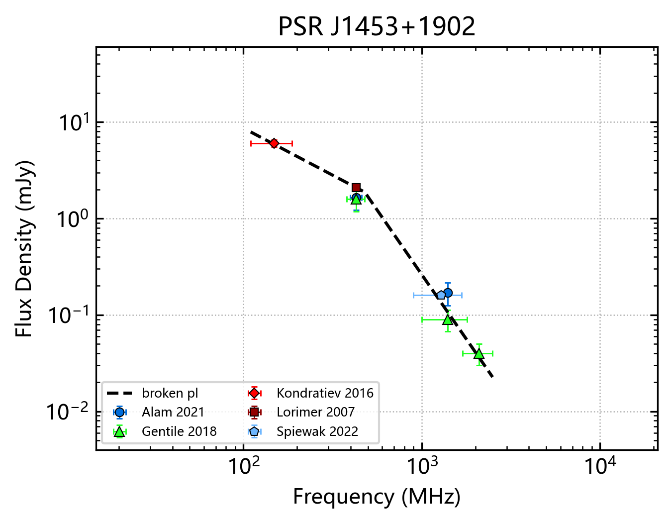
Figure 2: Broken power law model; Black dashed line: the best- fitting model to the data.

(iii)Power law with low-frequency turn-over:

$$S_{\rm\nu}=c\left(\frac{\nu}{\nu_{\rm 0}}\right)^{\alpha}\exp\left[\frac{\alpha}{\beta}\left(\frac{\nu}{\nu_{\rm peak}}\right)^{-\beta}\right],$$ (3)

where $\alpha$ is the spectral index, $\nu_{\rm peak}$is the turn-over frequency, and $0<\beta\leq 2.1$ determines the smoothness of the turn-over.

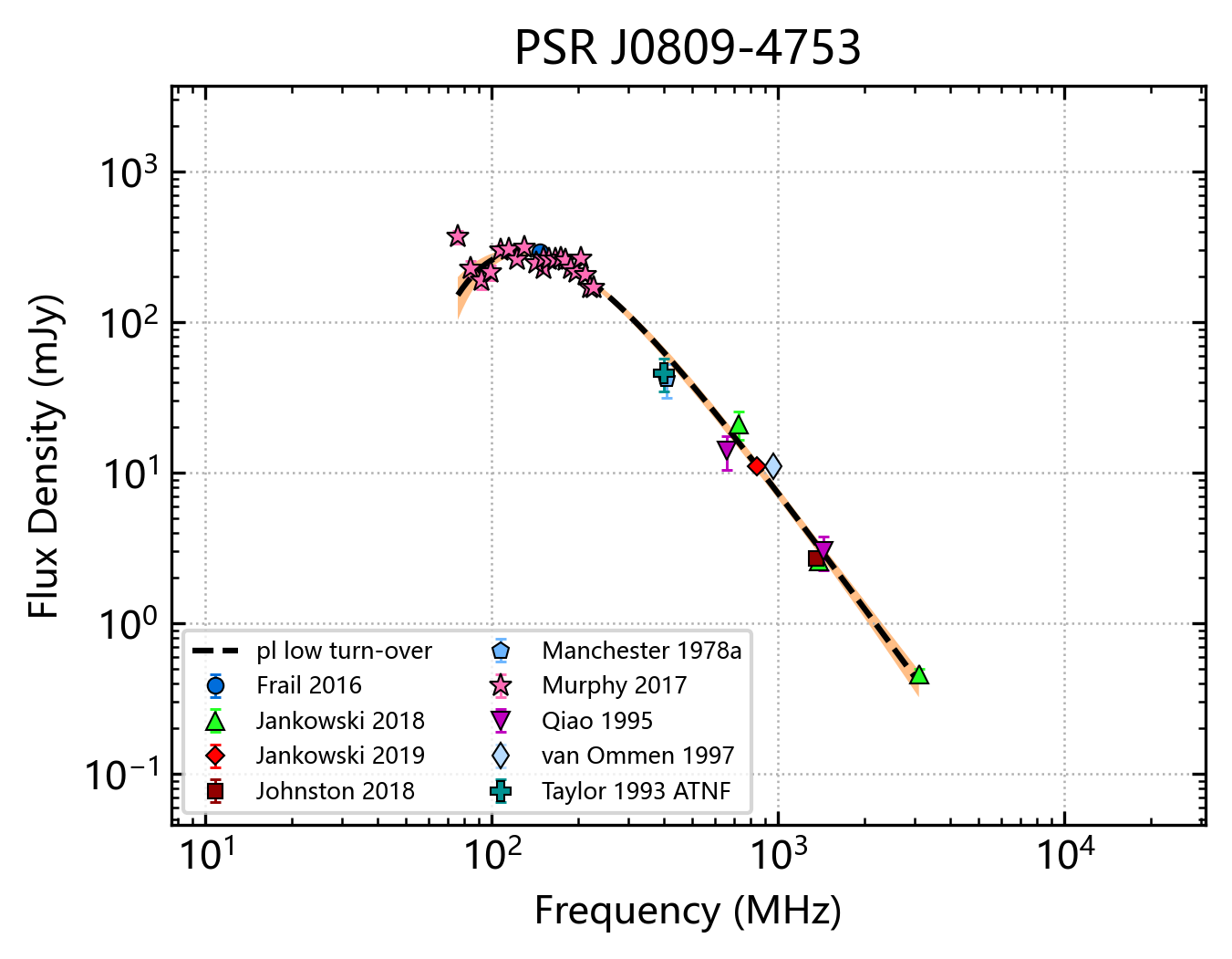
Figure 3: Low-frequency turn-over law model; Black dashed line: the best- fitting model to the data. Orange shaded envelope: the 1$\sigma$ uncertainty of the best-fitting model.

(iv)Power law with high-frequency cut-off:

$$S_{\rm\nu}=c\left(\frac{\nu}{\nu_{\rm 0}}\right)^{\alpha}\left(1-\frac{\nu}{\nu_{\rm c}}\right),\qquad\nu<\nu_{\rm c},$$ (4)

where $\alpha$ is the spectral index and $\nu_{\rm c}$ is the cut-off frequency.

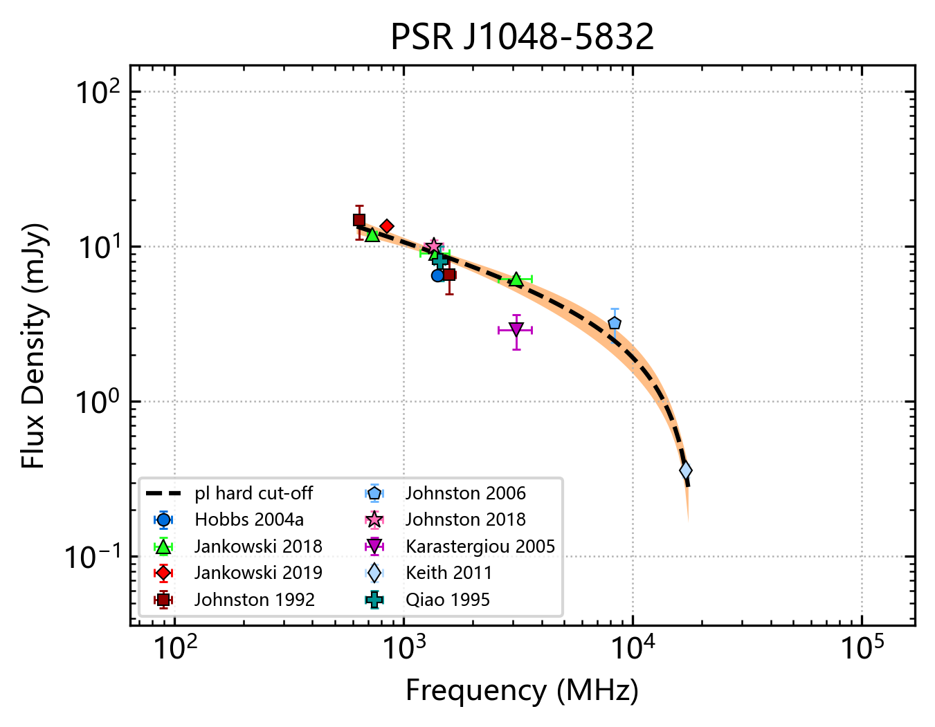
Figure 4: High-frequency cut-off model; Black dashed line: the best- fitting model to the data. Orange shaded envelope: the 1$\sigma$ uncertainty of the best-fitting model.

(v)Power law with double-turn-over:

$$S_{\rm\nu}=c\left(\frac{v}{\nu_{\rm 0}}\right)^{a}\left(1-\frac{v}{\nu_{\rm c}}\right)\exp\left[\frac{a}{\beta}\left(\frac{v}{\nu_{\rm c}}\right)^{-\beta}\right],\quad\nu<\nu_{\rm c},$$ (5)

where $\alpha$ is the spectral index, $\nu_{\rm peak}$ and $\nu_{\rm c}$ are the turn-over frequency and the cut-off frequency, respectively, and $0<\beta\leq 2.1$ determines the smoothness of the turn-over.

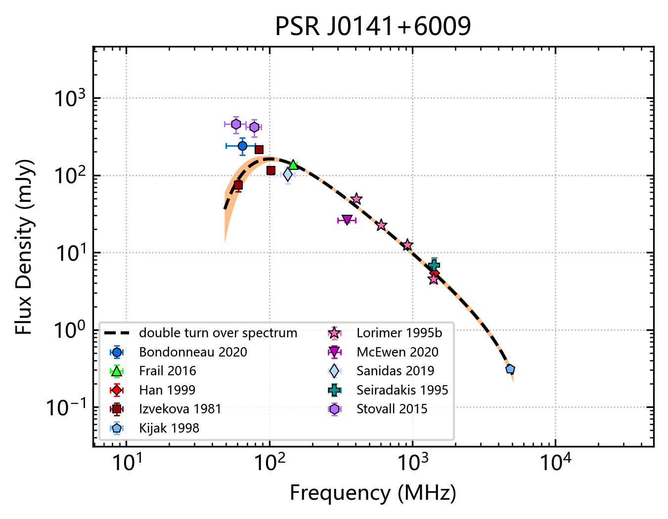
Figure 5: Double-turn-over law mode; Black dashed line: the best- fitting model to the data. Orange shaded envelope: the 1$\sigma$ uncertainty of the best-fitting model.

Since the extended data compiled from different studies were obtained by various telescopes with different calibration programs and observation frequencies, errors are unavailable for certain flux density values, resulting in visible deviations in the modeling of certain pulsars. Despite this, we treated such unmodelable pulsars as integral to the database’s completeness, and we anticipate an improvement in the process through the collection of pertinent data or the updating of software.

To enhance the accuracy of the spectral index of pulsars, it is necessary to ensure that each pulsar includes flux density values at the four distinct frequencies. Accordingly, we chose 941 pulsar samples out of a selection of more than 3300 pulsars that satisfy this requirement. Next, pulsar_spectra was employed to perform data modeling. pulsar_spectra applies the five models to each pulsar, subsequently determining the final model. However, some pulsars cannot be fitted well by pulsar_spectra. We separately fitted this portion of the data using a simple power law and provided an approximate spectral index. The fitting results for this portion are shown in A5. As a result, we performed a comprehensive analysis of the spectral information including 886 pulsars.

3 Results and analysis

Table 2: The distribution of different spectral models in normal pulsars and millisecond pulsars. The first column represents the five models we have used. The second and fourth columns indicate the number of normal pulsars and millisecond pulsars in each model respectively. The following third and fifth columns represent the percentage of the pulsars corresponding to each model.

Set	Normal pulsars	percentage	MSP	percentage
Simple power-law model	553	69.13	54	62.79
Broken power law model	45	5.63	9	10.47
High-frequency cut-off models	100	12.50	7	8.14
Low-frequency turn-over models	86	10.75	9	10.47
Double turn-over model	16	2.00	7	8.14
Total	800	-	86	-

Among the identified pulsars, around 90% of sources correspond to normal pulsars, amounting to a total number of 800. The majority, at 69.13%, obey the simple power-law model, while 12.50% and 10.75% conform to the high-frequency cut-off and low-frequency turn-over models, respectively. The least eligible models are the broken power-law model and double turn-over model with amounting to merely 5.63% and 2.00% of the total, respectively. Millisecond pulsars constitute roughly 10% of the entire population with 86 identified instances. Within this subset, the simple power-law model retains the highest correlation coefficient at 62.79%, followed by the broken power-law and low-frequency turn-over models, both being 10.47%, and finally, the high-frequency cut-off and double turn-over models at 8.14%(see Table 2). We presented our investigation of the non-simple power law models in tables, with LABEL:tab:a1 offering insights on the broken power law model and LABEL:tab:a3 showing the low-frequency turn-over model results. LABEL:tab:a4 and A4 detailed the findings of high-frequency cut-off and the double turn-over models, respectively. We also mark the MSPs with asterisk in the table. Particularly, we present the spectral analysis of GPS pulsars in Section 3.3. According to Kijak et al. (2011), GPS pulsars are believed to be relatively young and have high dispersion measures (DM), which may be related to their surrounding environment.

3.1 Normal pulsars

3.1.1 Simple power-law model

we have identified a total of $553$ normal pulsars which can be effectively modeled using a simple power-law. The corresponding spectral histogram of the resulting analysis, is shown in Figure 6.

We calculated the average spectral index of $-1.57\pm 0.32$ by weighting their reciprocal errors for each pulsar, and estimated the uncertainty by standard deviation. The weighted mean spectral index from Jankowski et al. (2018) is consistent with our results within uncertainties. In addition, we constructed a kernel density estimation (KDE) plot(green line) and a Gaussian fitting(red line) in Figure 6. It is worth noting that eleven normal pulsars show positive spectral indices, excluding the pulsar PSR J1745-2900 for which high-frequency data is lacking. Furthermore, we performed the KS test and obtained a p-value of $0.18$.

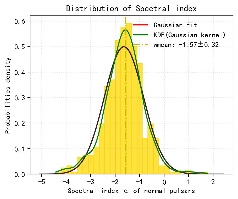
Figure 6: Histogram of the spectral indices $\alpha$ for normal pulsars that were classified to have simple power-law. We display a Gaussian and a kernel density estimation (KDE) using a Gaussian kernel fit to the data with a red and green line. We show a weighted mean spectral index(wmean: $-1.57\pm 0.32$).

3.1.2 Broken power-law spectra model

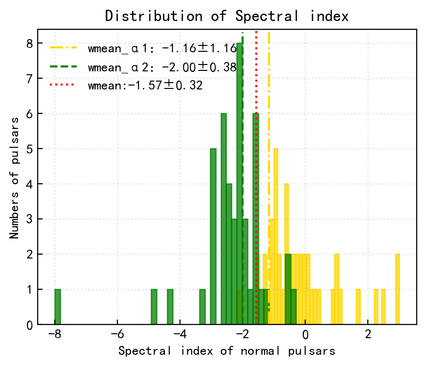
Figure 7: Histogram of the spectral indices $\alpha$ for normal pulsars that were classified to have broken power-law. Among them, green and yellow represent the spectral indices before and after the break, respectively. The corresponding dashed lines of the colors represent the corresponding weighted averages. In addition, we specifically use a red dashed line to represent the weighted average of normal pulsars in the simple power-law model.

The broken power-law model was a rare occurrence, with only $5.63\%$ of the normal pulsars in Figure 7 exhibits such a behaviour. Based on the fitting results, histograms of the spectral indices were plotted. The weighted average spectral indices before and after the broken are $-1.16\pm 1.16$ and $-2.00\pm 0.38$, respectively.

Furthermore, to discuss the location of spectral breaks, we constructed a frequency histogram at the points of spectral breaks in Figure 8. The results reveal that all pulsars, except for J1705-1906 at $4850$ MHz and J1935+1616 at $2291$ MHz, exhibit spectral breaks below $2$ GHz. Upon examination of the break frequencies, the median value (dashed line) is observed $692$ MHz. The maximum position of the spectral break is $4850$ MHz, and the minimum is $100$ MHz. Consequently, it can be seen from the figure that the breaks are mainly concentrated within the $100$ MHz to $1$ GHz range.

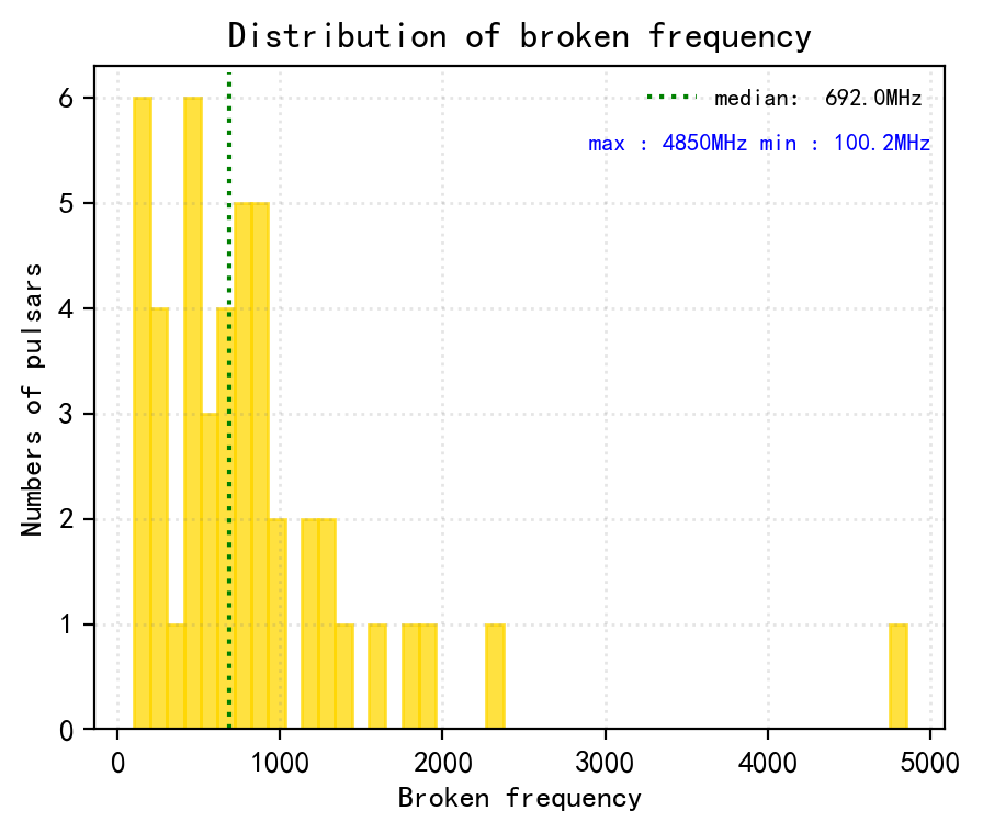
Figure 8: The frequency histogram at the points of spectral breaks. We have marked the position of the median with a dashed line in the figure, and provided its value, as well as the maximum and minimum values, in the upper right corner.

Figure 9 shows a scatter plot of the ratio between the spectra before and after the spectral break against the position of the break. Since some pulsars exhibit positive spectral indices before the break but negative spectral indices after the break, the graph can be divided into four regions. These regions, delimited by solid and dashed red lines, are determined by the spectral index ratio. Within the range of -1 to 1, a total of 33 pulsars have spectral indices that get flatten after the break, while the remaining pulsars exhibit steeper spectral indices. Notably, among the 14 pulsars with negative values, their spectral indices transition from positive to complex values, indicating a flipping behavior in their spectral behavior. Therefore, the broken power-law model reveals three distinct spectral behaviour patterns. Among these patterns, 29 pulsars exhibit flatter spectral indices after the break, while 2 pulsars exhibit steeper spectral indices. The remaining 14 pulsars display a flipping behavior in their spectral indices.

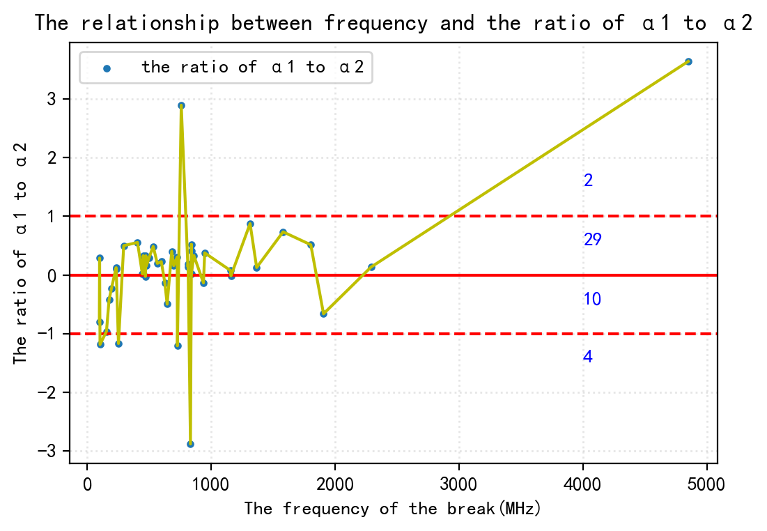
Figure 9: The relationship between frequency and the ratio of $\alpha_{1}$ to $\alpha_{2}$, where $\alpha_{1}$ and $\alpha_{2}$ are the spectral indices before and after the break. The blue numbers indicate the number of pulsars in each region.

3.1.3 Power-law spectra with low-frequency turn-over model

The PULSAR-SPECTRA model employs a synchrotron radiation function to describe the low-frequency turn-over process (Izvekova et al., 1981), but can describe the spectra expected due to both synchrotron self and thermal free–free absorption. In this model, a variable $\beta$ is utilized as an unspecified parameter, which determines the smoothness of the turn-over; when it equals to $2.1$, $\beta$ can represent free-free absorption, as indicated by Rajwade et al. (2016) and Kijak et al. (2017). Therefore, the outcomes of the low-frequency turn-over model indicate that approximately $41.8\%$ of absorption results from a free-free absorption model. we specifically used the Kolmogorov-Smirnov test to analyze the distribution of spectral indices in these two scenarios. The results indicate that they originate from different distributions.

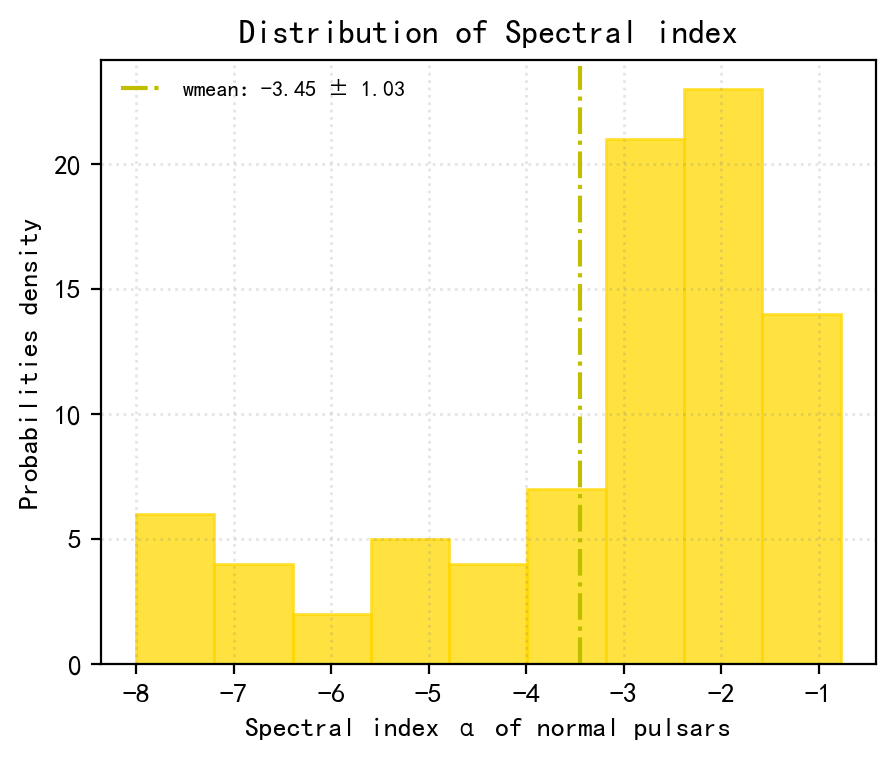
Figure 10: Histogram of the spectral indices $\alpha$ for normal pulsars that were classified to have low-frequency turn-over. The dashed line represents the weighted average.

In terms of the distribution of spectral indices (as shown in Figure 10), the low-frequency turn-over has a weighted average of $-3.59\pm 1.13$ indicating a smaller value in contrast to typical spectral index values. Additionally, concerning the turn-over frequency distribution (shown in the Figure 11), the maximum frequency recorded was $1998.4$ MHz, and the minimum frequency was $41.6$ MHz. The median frequency recorded was $235$ MHz (dashed line). This value is closer to the minimum value rather than the maximum value, indicating that the locations of low-frequency turn-over are more concentrated below 235 MHz.

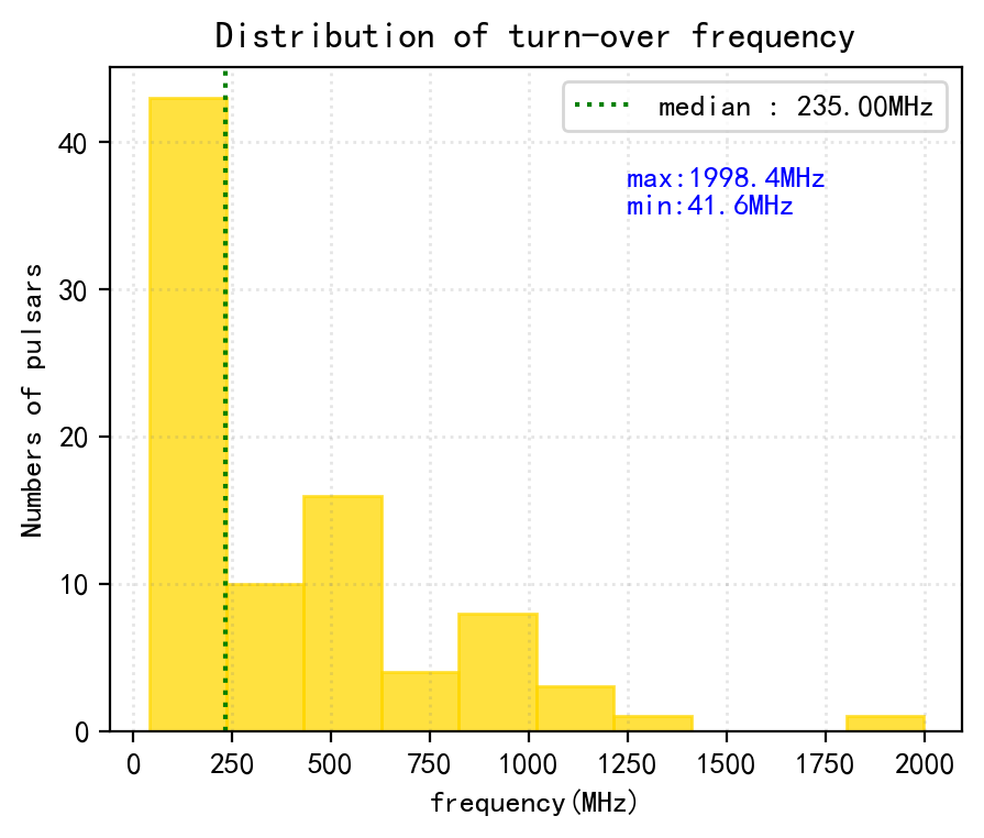
Figure 11: Distribution of turn-over frequency. We also have marked the position of the median with a dashed line in the figure, and provided its value, as well as the maximum and minimum values, in the upper right corner.

3.1.4 Power-law spectra with high-frequency cut-off model

Of the 800 normal pulsars in the sample, $12.50\%$ are part of the high-frequency cut-off model, which is the most common model apart from the simple power-law model. A histogram of the spectral index shown in Figure 12 revealed an average weight of $-0.73\pm 0.64$4, with a range from $-2$ to $0$.

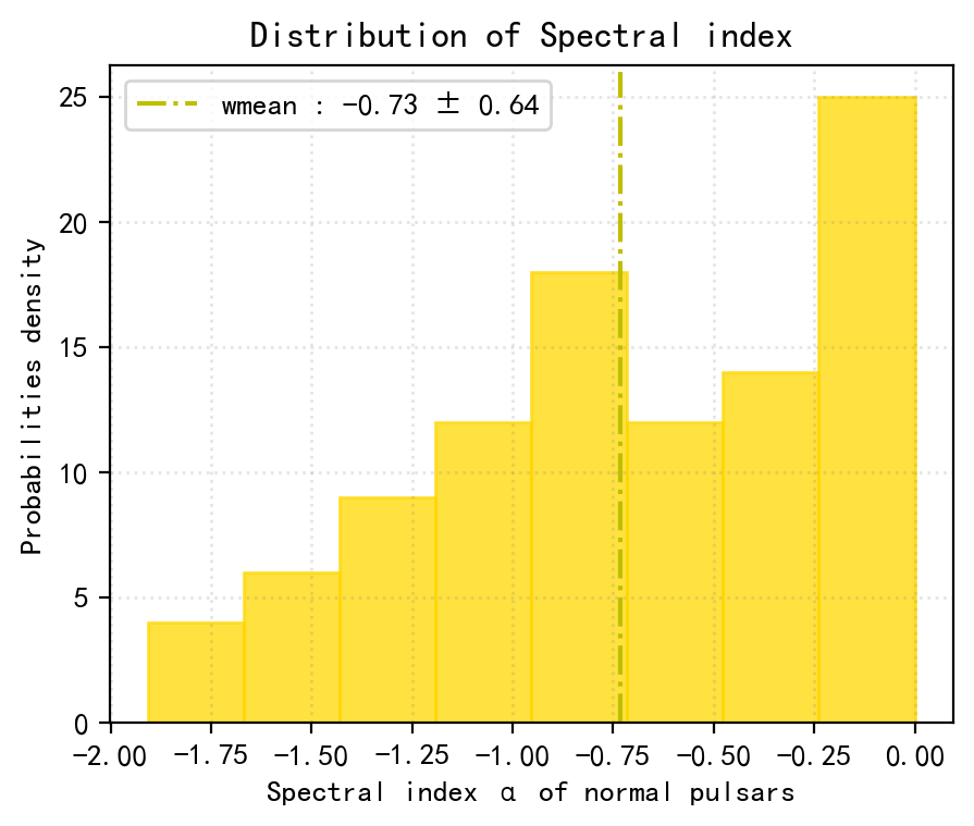
Figure 12: Histogram of the spectral indices $\alpha$ for normal pulsars that were classified to have high-frequency cut-off. The dashed line represents the weighted average.

The cut-off frequency of pulsars is generally below $15$ GHz, as shown in Figure 13. However, there are exceptions like PSRs J1048–5832, J1721–3532, and J1709-1640, with J1709-1640 having the highest cut-off frequency of $25.3$ GHz. The graph clearly indicates a higher concentration below 10 GHz for the high-frequency cut-off, with the median position at 3392 MHz. We observe that three pulsars with the largest cut-off frequencies exhibit characteristics indicative of youth and stronger magnetic field intensities compared to the majority of pulsars. Specifically, of the three pulsars examined in this study, the youngest is PSR J1048-5832, estimated to be 20,400 years old, making it the second youngest pulsar in the model. Even the oldest pulsar, PSR J1709-1640 with an age of merely 1.64 million years, is younger than more than half of the pulsars included in this model. They posses larger magnetic field strength compared to approximately seventy percent of the pulsars in our sample.

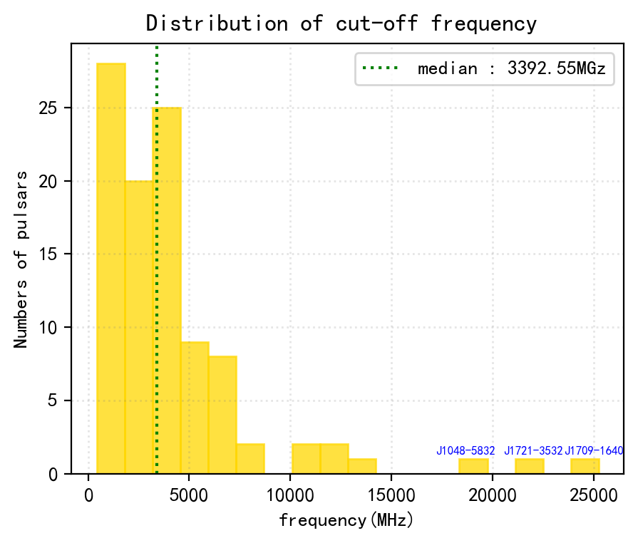
Figure 13: Distribution of cut-off frequency. We have marked the position of the median with a dashed line in the figure, and provided its value. The three pulsars exhibiting the largest cut-off frequencies are identified as J1048-5832, J1721-3532, and J1709-1640.

3.1.5 Double-turn-over spectrum model

The double-turn-over model simultaneously includes a low-frequency turn-over and a high-frequency cut-off phenomena. This particular model has the smallest correlation coefficient among the five models, just making up approximately $2.00\%$ of the total. They exhibit a weighted average $-2.21\pm 2.06$ of spectral index as observed from the spectral index in Figure 14.

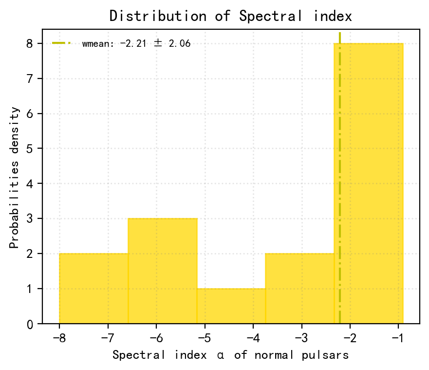
Figure 14: Histogram of the spectral indices $\alpha$ for normal pulsars that were classified to have Double-turn-over spectrum. The dashed line represents the weighted average.

In addition, we separately discussed the correlation between spectral indices and characteristic parameters for each model. The results shown in Table 3 indicate that there is no strong correlation between spectral indices and characteristic parameters by means of any model. We also analyzed the correlation between the spectral index and the characteristic parameters of all normal pulsars. Specifically, for the broken power-law model, we separated the spectral index into two parts: before and after the break. We then considered them as separate spectral indices for two individual power-law models. Figure 15 presents the corresponding results.

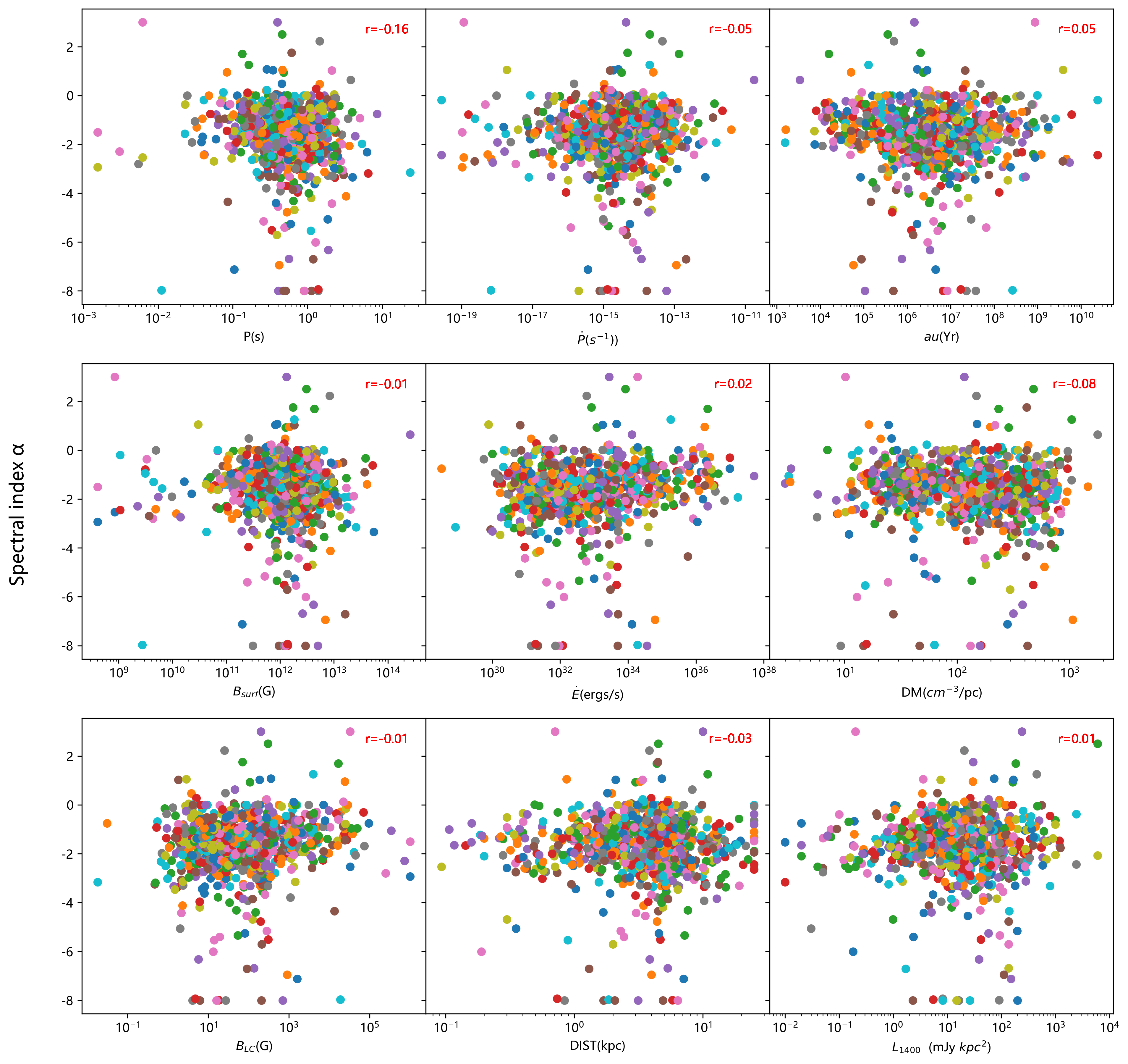
Figure 15: Distributions of spectral index $\alpha$ of normal pulsars vs pulsar period $P$, period derivative $\dot{P}$, characteristic age $\tau$, 1400 MHz pseudo-luminosity $L_{\rm{1400}}$, dispersion measure (DM), surface magnetic field $B_{\rm{\text{surf}}}$, the pulsar distance (DIST), Magnetic field at light cylinder $B_{\rm{\text{LC}}}$, spin-down luminosity $\dot{E}$.. The parameters of the fit and the Spearman rank coefficient are given at the top right corner of each subplot.

Table 3: Correlations between the intrinsic parameters of normal pulsars and the spectral indices across various models, along with the corresponding $p_{\rm values}$. In this study, we find no significant correlation between the spectral index of normal pulsars and their characteristic parameters, both at the overall level and in terms of individual models.

Parameters1	sim	bro		dou	low	high	Total 2
P	-0.20 (0.00)	-0.04 (0.80)	-0.42 (0.00)	-0.18 (0.50)	-0.11 (0.32)	-0.06 (0.54)	-0.16 (0.00)
$\dot{P}$	-0.07 (0.10)	0.10 (0.52)	-0.01 (0.97)	0.09 (0.75)	0.14 (0.21)	-0.01 (0.90)	-0.05 (0.14)
$\tau$	0.05 (0.22)	-0.10 (0.52)	-0.15 (0.32)	-0.23 (0.40)	-0.13 (0.23)	0 (0.99)	0.05 (0.17)
$B_{\rm{\text{surf}}}$	0 (0.97)	0.06 (0.71)	-0.16 (0.29)	0.03 (0.91)	0.07 (0.51)	-0.06 (0.56)	-0.01 (0.74)
$\dot{E}$	0.05 (0.26)	-0.18 (0.23)	0.10 (0.53)	-0.25 (0.35)	0.01 (0.93)	0.09 (0.38)	0.02 (0.54)
DM	-0.10 (0.02)	0.16 (0.30)	-0.11 (0.49)	-0.21 (0.43)	-0.14 (0.21)	0.07 (0.48)	-0.05 (0.03)
$B_{\rm{\text{LC}}}$	-0.03 (0.50)	0.06 (0.71)	0.33 (0.03)	0.17 (0.52)	0.09 (0.42)	0.01 (0.56)	-0.01 (0.83)
Dist	-0.09 (0.03)	0.11 (0.46)	-0.10 (0.51)	-0.49 (0.05)	-0.17 (0.12)	0.15 (0.15)	-0.03 (0.33)
$L_{\rm{1400}}$	0.07 (0.10)	0.13 (0.38)	0.04 (0.80)	-0.11 (0.68)	-0.04 (0.73)	-0.18 (0.07)	0.01 (0.74)

• Pulsar characteristic parameters : pulsar period $P$, period derivative $\dot{P}$, characteristic age $\tau$, 1400 MHz pseudo-luminosity $L_{\rm{1400}}$, dispersion measure (DM), surface magnetic field $B_{\rm{\text{surf}}}$, the pulsar distance (DIST), Magnetic field at light cylinder $B_{\rm{\text{LC}}}$, spin-down luminosity $\dot{E}$.

• Here, abbreviations are used for the names of the models, and the names after the abbreviations are indicated in parentheses: the simple power law(sim), broken power law(bro), double tur-nover spectrum(dou), low-frequencies turn-over(low) and high-frequencies cut-off(high). The last column represents all normal pulsars without distinguishing the models.

3.2 Millisecond pulsars(MSP)

Table 4: Correlations between the intrinsic parameters of millisecond pulsars (MSPs) and the spectral indices across various models, along with the corresponding $p_{\rm values}$. In line with normal pulsars, no significant correlation is observed between the spectral index and the characteristic parameters at the overall level. However, for individual models, with the exception of the simple power-law model, a noteworthy correlation is observed between the spectral index and certain characteristic parameters. To emphasize this finding, we have highlighted the relevant coefficients. Bold font indicates that the absolute value of correlation is greater than 0.5.

Parameters1	sim	bro		dou	low	high	Total 2
P	0.12 (0.39)	-0.5 (0.17)	-0.52 (0.15)	0.75 (0.05)	0.15 (0.70)	-0.14 (0.76)	0.03 (0.75)
$\dot{P}$	0 (0.99)	0.05 (0.90)	-0.12 (0.77)	0.71 (0.07)	0.48 (0.19)	0.36 (0.43)	0.06 (0.56)
$\tau$	-0.24 (0.08)	-0.07 (0.86)	-0.37 (0.33)	-0.71 (0.07)	-0.26 (0.50)	-0.71 (0.07)	0.24 (0.02)
$B_{\rm{\text{surf}}}$	0.02 (0.88)	-0.13 (0.75)	-0.19 (0.62)	-0.43 (0.34)	-0.68 (0.04)	-0.14 (0.76)	-0.07 (0.50)
$\dot{E}$	-0.09 (0.51)	0.40 (0.29)	-0.60 (0.09)	-0.61 (0.15)	-0.24 (0.53)	0.46 (0.29)	-0.11 (0.28)
DM	-0.35 (0.01)	-0.18 (0.64)	-0.32 (0.41)	-0.64 (0.12)	0.04 (0.91)	0.39 (0.38)	-0.26 (0.01)
$B_{\rm{\text{LC}}}$	-0.12 (0.39)	0.5 (0.17)	0.57 (0.11)	-0.07 (0.88)	-0.46 (0.21)	0.32 (0.48)	-0.13 (0.23)
Dist	-0.44 (0.00)	0.6 (0.09)	0.02 (0.97)	-0.57 (0.18)	-0.61 (0.08)	0.57 (0.18)	-0.31 (0.00)
$L_{\rm{1400}}$	-0.11 (0.43)	0.02 (0.97)	0.48 (0.19)	0 (1.00)	-0.27 (0.49)	0.79 (0.04)	0.00 (0.97)

• Pulsar characteristic parameters : pulsar period $P$, period derivative $\dot{P}$, characteristic age $\tau$, 1400 MHz pseudo-luminosity $L_{\rm{1400}}$, dispersion measure (DM), surface magnetic field $B_{\rm{\text{surf}}}$, the pulsar distance (DIST), Magnetic field at light cylinder $B_{\rm{\text{LC}}}$, spin-down luminosity $\dot{E}$.

• Here, abbreviations are used for the names of the models, and the names after the abbreviations are indicated in parentheses: the simple power law(sim), broken power law(bro), double turn-over spectrum(dou), low-frequencies turn-over(low) and high-frequencies cut-off(high). The last column represents all MSPs without distinguishing the models.

The criteria for identifying millisecond pulsars are established in Lorimer (2008). It is specified so that millisecond pulsars should have periods ranging from $1.4$ ms to $30$ ms, and their period derivatives should be less than $10^{-19}$ s/s. Based on these criteria, we selected 86 MSPs, whose spectral behavior was also described with the five models employed above. Among these pulsars, $62.79\%$ can be adequately represented using a simple power law model. The remaining millisecond pulsars exhibit a nearly uniform distribution among the other models. As shown in Table 2, the correlation coefficient of the power-law model and the low-frequency turn-over is approximately 10.47%, while the correlation coefficients of the high-frequency cut-off and double turn-over model are both 8.14%.

3.2.1 Simple power-law model

The overall trend of the millisecond pulsar spectral index remains consistent with a normal distribution, with the weighted average of $-1.89\pm 0.21$. For millisecond pulsars other than $J1802-2124$ ($0.042$), $J2017+0603$ ($1.036$), and $J2215+5135$ ($-3.702$), the spectral index generally ranges from $-3$ to $0$.

3.2.2 Broken power-law spectra model

There are 9 millisecond pulsars (MSPs) that conform to the broken power-law model. The millisecond pulsars’ spectral indices before the break range from $-1.79$ to $0.937$, with a weighted average of $-1.12$. After the break, the spectral indices are distributed between $-2.827$ and $-0.007$, with a weighted average of $-2.48$. However, for J1918-0642, the spectral index reaches $-8$ after the break, which is in close proximity to our predefined lower fit limit.

When discussing the correlation between the spectral index and characteristic parameters, millisecond pulsars exhibit broader differences compared to the normal pulsars in Table 4. Notably, the correlation between the spectral index before the break and the pulsar distance represents a value of $0.60$. Similarly, the correlation between the spectral index after the break and the spin-down energy loss rate also indicates a value of $0.60$.

3.2.3 Power-law spectra with low-frequency turn-over

Additionally, there are 9 millisecond pulsars (MSPs) that conform to the low-frequency turn-over model. Overall, the weighted average spectral index is significantly low, measuring $-5.54$. J$0024-7204C$ and J$0024-7204$ exhibit a spectral index of $-8$, whereas J$1600-3053$ has a spectral index of $-7.572$. Based on the frequency distribution, it is evident that the breaks exhibit a notable concentration within the $100$ MHz to $1$ GHz range.

Moreover, we have examined the correlations between the spectral index and characteristic parameters of pulsars. The results reveal a strong negative correlation of $-0.68$ between the spectral index and the intensity of the magnetic field, as well as a negative correlation of $-0.61$ between the spectral index and the distance of the pulsars. Moreover, we noticed a positive correlation of $0.48$ between the spectral index and the period derivative, and a negative correlation of $-0.46$ between the spectral index and the magnetic field intensity at the light cylinder (see Table 4). The results may be an indicative of evolution of the millisecond pulsars in low mass X-ray binaries (LMXBs). In the Roche lobe overflow phase of LMXBs, matter carrying high specific angular momentum from a low mass companion star is transferred onto the neutron star through an accretion disk, leading to acceleration of rotation of the underlying neutron star. Also settled matter in the form of highly conductive plasma causes magnetic field to decay by heating up the surface of the neutron star (Shibazaki et al., 1989) and shielding the field lines via diamagnetic screening effect (Choudhuri & Konar, 2004). If this binary evolution stage lasts for $\lesssim$ Gyr, that neutron star ends up with a millisecond pulsar attaining fast rotation close to the maximum possible equilibrium period with a residual magnetic field. As a consequence of such evolution, the millisecond pulsars possess a narrow range both for $P$, $\dot{P}$ and $B_{\rm LC}$ compared to the radio pulsar population, which may be the underlying reason for the corresponding correlations.

3.2.4 Power-law spectra with high-frequency cut-off

A total of 7 millisecond pulsars have been included in the high-frequency cut-off model. The distribution of their spectral indices is concentrated, ranging between $-1.374$ and $0$, with a weighted average spectral index of $-1.02$. Looking at the cut-off positions, except J$1810+1744$ at $416$ MHz, all millisecond pulsars have cut-off frequencies above $1.5$ GHz. Additionally, under this spectra fitting model, the correlation coefficients between millisecond pulsars’ spectral index and characteristic age and radio luminosity at $1400$ MHz, are $-0.71$ and $0.79$, respectively. The correlation coefficient between millisecond pulsars’ spectral index and their distance reaches $0.57$ (see Table 4).

3.2.5 Double-turn-over spectrum model

Seven millisecond pulsars conforming to the double reversal model were identified, all with spectral indices below $0$ and a weighted average $-2.82\pm 2.58$. Among these pulsars, $J1911-1114$ exhibits the smallest spectral index of $-8$. With the exception of $J0024-7204D$ at $689.5$ MHz, the peak frequencies of these pulsars are all below $200$ MHz, while the cut-off positions for the spectral indices are above $4$ GHz.

Moreover, a closer examination revealed strong correlations between spectral indices and characteristic parameters (see Table 4), including period, period derivative, and characteristic age, with correlation coefficients of $0.75$, $0.71$, and $-0.71$. Additionally, the spectral index shows significant correlations with spin-down power ($-0.61$), dispersion measure ($0.64$), and pulsar distance ($-0.57$).

Finally, we analyzed the correlation between the spectral index and the characteristic parameters of all millisecond pulsars, just like in the previous section. The final results are shown in Figure 16. Overall, there is not a strong correlation observed.

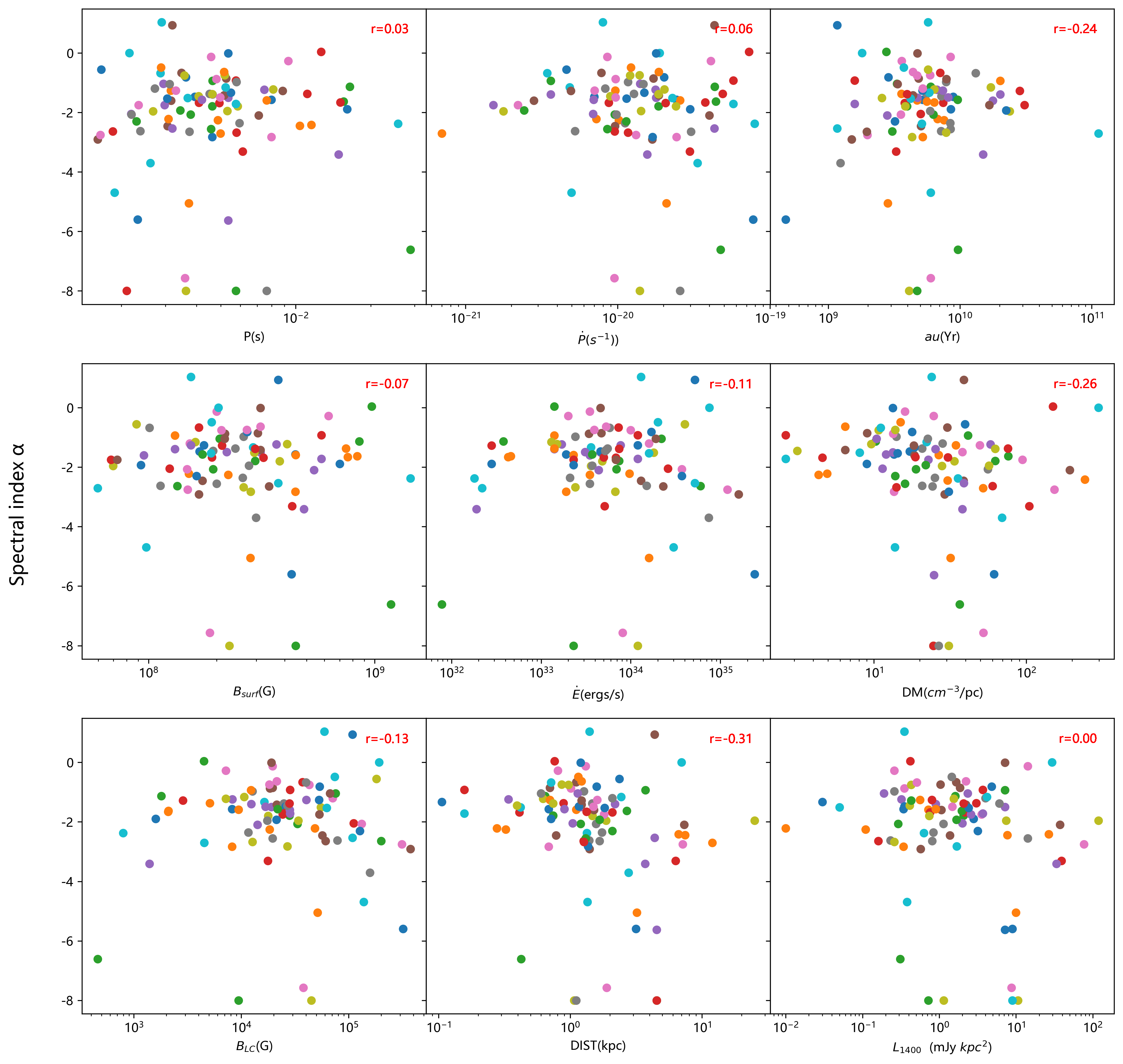
Figure 16: Distributions of spectral index $\alpha$ of MPSs vs pulsar period $P$, period derivative $\dot{P}$, characteristic age $\tau$, 1400 MHz pseudo-luminosity $L_{\rm{1400}}$, dispersion measure (DM), surface magnetic field $B_{\rm{\text{surf}}}$, the pulsar distance (DIST), Magnetic field at light cylinder $B_{\rm{\text{LC}}}$, spin-down luminosity $\dot{E}$. The parameters of the fit and the Spearman rank coefficient are given at the top right corner of each subplot.

3.3 The gigahertz-peaked spectrum(GPS)

The criteria set by Jankowski et al. (2018) was used to identify GPS pulsars, whereby pulsars displaying peak frequencies between $0.6$ and $2$ GHz were selected, without considering the best-fit models. From our analysis, 33 GPS pulsars meet these criteria, with only $11$ previously identified (see Table 5). Notably, of the newly identified GPS pulsars, $4$ showed spectral breaks, $16$ exhibited the low-frequency turn-over feature, while $2$ appeared in double-turn-over models.

We compared our results with those of Kijak et al. (2021) and discovered that $22$ pulsars did not satisfy our GPS criteria. Specifically, only $4$ GPS pulsars have flux density values at three frequencies, thereby failing to fulfill our requirement that all the pulsars we are studying must provide four or more flux density values at different frequencies. Five of the pulsars exhibited peak frequencies below $600$ MHz, while seven others obeyed to a simple power-law model, and the remaining six utilized high-frequency cut-off models. We excluded these models from our GPS pulsars because they did not conform with our "peak" criteria.

Statistical analysis was performed on the confirmed 33 GPS pulsars, of which only approximately two-thirds exhibited high dispersion measures ($\text{DM}>150\,\text{cm}^{-3}\,\mathrm{pc}$). We also investigated the correlation between $v_{\text{peak}}$ and various characteristic parameters of the pulsars. The correlation with DM was found to be weak ($r=0.20$), providing further support for the hypothesis proposed by (Kijak et al., 2007) that the occurrence of higher DM values in GPS pulsars is due to selection effects. Additionally, the results revealed a significant correlation between $v_{\text{peak}}$ and both the period ($r=0.40$) and the period derivative ($r=0.49$). Furthermore, a weak negative correlation was observed between $v_{\text{peak}}$ and the characteristic age ($r=-0.05$).

Table 5: Some parameters of GPS pulsars, where $\nu_{p}$ and $\nu_{p}$_err are the the peak/turn-over frequency and its error, $P$ is the pulsar period , $\dot{P}$ is the period derivative, $\tau$ is the characteristic age, DM is the dispersion measure.

PSRJ1	model2	$\nu_{p}*$ (MHz)	$\nu_{p}$_err (MHz)	P (s)	$\dot{P}$ (s/s-1)	DM (cm-3 pc)	$\tau$ (yr)
J0024-7204C	low	600.4	9	5.76E-03	-4.99E-20	24.5955	*
J0024-7204D	dou	689.5	40.6	5.36E-03	-3.42E-21	24.7432	*
J0024-7204J	low	607.8	4.5	2.10E-03	-9.79E-21	24.5932	*
J0908-4913	low	603.5	42.3	1.07E-01	1.51E-14	180.44	112000
J1326-5859	bro	647.1	201.7	4.78E-01	3.2418E-15	287.17	2340000
J1513-5908	low	611.6	65.6	1.52E-01	1.53E-12	252.5	1570
J1524-5706	low	1189.4	65.2	1.12E+00	3.56E-13	832	49600
J1600-3053	low	847	18.7	3.60E-03	9.50E-21	52.3282	6000000000
J1635-5954	low	857.2	59.9	5.29E-01	1.37E-15	134.9	6130000
J1644-4559	bro	729.9	3	4.55E-01	2.00892E-14	478.66	359000
J1705-3950	low	1039.4	71.9	3.19E-01	6.06E-14	207.25	83400
J1727-2739	bro	939.9	231.6	1.29E+00	1.07E-15	146	19100000
J1740-3015	low	951.4	146.7	6.07E-01	4.66E-13	151.96	20600
J1741-3016*	dou	947.9	26.3	1.89E+00	8.99E-15	382	3340000
J1745-3040	low	1009.9	130.2	3.67E-01	1.07E-14	88.373	546000
J1751-3323	low	1006.2	109.3	5.48E-01	8.83E-15	296.7	984000
J1753-2501	low	760.8	91.1	5.28E-01	1.41E-14	672	593000
J1803-2137	bro	835.2	33.5	1.34E-01	1.34359E-13	233.99	15800
J1806-1154*	low	642.3	64.7	5.23E-01	1.41E-15	122.41	5880000
J1809-1917	bro	1908.2	231.1	8.28E-02	2.55302E-14	197.1	51400
J1818-1422*	low	886.1	54	2.91E-01	2.04E-15	619.65	2270000
J1823-1115*	bro	628.4	56.1	2.80E-01	1.37862E-15	428.59	3220000
J1825-1446*	dou	1722.7	223.8	2.79E-01	2.27E-14	352.23	195000
J1826-1334*	low	1220.1	134.6	1.01E-01	7.53E-14	231	21400
J1830-1059*	low	913.1	47.8	4.05E-01	5.99E-14	159.7	107000
J1832-1021*	dou	2000	1483.6	3.30E-01	4.20E-15	474.14	1250000
J1843-0459*	low	807.4	59.1	7.55E-01	8.54E-16	444.1	14000000
J1844-0244*	low	861.1	45.7	5.08E-01	1.67E-14	422.13	481000
J1844-0538*	low	1008	57.2	2.56E-01	9.71E-15	411.71	417000
J1845-0743*	low	804.5	9.1	1.05E-01	3.67E-16	280.93	4520000
J1852-0635*	low	1119	41.1	5.24E-01	1.46E-14	173.9	568000
J1918+1444*	low	1998.4	1640.8	1.18E+00	2.12E-13	27.202	88100
J2321+6024	bro	1161.7	66.9	2.26E+00	7.03689E-15	94.591	5080000

• The asterisk (*) represents GPS pulsars identified in previous literature.

• Here, abbreviations are used for the names of the models, and the names after the abbreviations are indicated in parentheses: broken power law(bro), double turn-over spectrum(dou) and low-frequencies turn-over(low)

4 DISCUSSION

Recently, there has been extensive research investigating the determination of flux and spectral indices of pulsars, nonetheless, there is still no definite explanation for the radiation mechanism and spectral turn-over phenomenon of pulsars. To understand these features better, it is essential to investigate pulsar flux density and the corresponding spectrum. Since the frequency dependence of pulsar emission is a crucial characteristics, the spectrum is intimately related to the radiative mechanism of pulsars. Such an understanding is especially crucial for examining the physical conditions in the magnetosphere. Therefore, the analysis of pulsar flux density and its spectral indices is essential for providing further insights into pulsars. Through sampling a larger group, we aim to investigate the similarities and differences in spectral indices between millisecond pulsars and normal pulsars.

4.1 Spectral indices of Normal pulsars and millisecond pulsars

Several reports on the average spectral indices of pulsars have been generated from the previous spectral studies. Sieber (1973) reported an average spectral index of approximately $-1.62$ after examining the spectral indices of $27$ pulsars known to that date. Kramer et al. (1998) suggested that the average spectral index of millisecond pulsars (MSPs) should be slightly steeper than that of ordinary pulsars, with being approximately $-1.8$. This value remains consistent with the average value of $-1.8\pm 0.2$ from the simple power-law fit reported by Maron et al. (2000). Additionally, Malofeev et al. (1994) noted that pulsars with spectral turn-over typically demonstrate a low-frequency turn-over at approximately $0.1$ GHz and a high-frequency cut-off frequency ranging from $0.4$ to $9.1$ GHz. These pulsars exhibit a steeper spectral index after the turn-over. The results from analysis our sample suggest that the spectral index shows a steeper trend after a spectral break in the broken power-law model, regardless of whether they are normal pulsars or MSPs. In a recent study, Spiewak et al. (2022) reported an average spectral index of approximately $-1.9$ for $189$ MSPs. More recently, a more specific study of flux densities and spectral indices of MSPs with MeerKAT has been done by Gitika et al. (2023). They reported a mean spectral index of $-1.86(6)$ for $89$ MSPs. This value appears to be close to the previous results. Our simple power-law model produced a similar average spectral index of approximately $-1.61$, which is comparable to the reported average spectral index of $276$ pulsars by Jankowski et al. (2018). Further analysis reveals that only about $29$% of our sample overlaps with Jankowski et al. (2018)’s dataset. This indicates that the average spectral index is relatively independent to a large extent.

The weighted average of the spectral index from each model reveals that, except for the broken power-law model, millisecond pulsars exhibit steeper spectral index compared to normal pulsars in the other models in Table 6. The results here are consistent with those reported in Lorimer et al. (1995), where millisecond pulsars exhibit steeper spectral indices than normal pulsars. They argue that this may be caused by the characteristic age of pulsars. As is shown in the subsequent section, an analysis of the correlation between the spectral index and characteristic ages of millisecond pulsars revealed no significant conformity. A comparison of the different models reveals that both millisecond pulsars and normal pulsars exhibit the lowest spectral index in the low-frequency turn-over model, followed by the double turn-over model, the simple power-law model, and finally the high-frequency cut-off model. However, in the case of the broken power-law model, if we consider only the spectral index before the spectral break, it emerges out as the second highest. This phenomenon could arise from various spectral behavior patterns or other factors that influence the spectral index. These factors may include specific characteristics of pulsars, such as their period and characteristic age.

Table 6: Weighted average of normal pulsars and millisecond pulsars under different models.

model1	Normal pulsars	MSPs
simple power-law	-1.57±0.32	-1.65±0.81
broken power-law 2	-1.16±1.16 -2.00±0.38	-1.12±0.65 -1.75±0.38
low-frequency turn-over	-3.45±1.03	-5.54±1.80
high-frequency cut-off	-0.73±0.64	-1.02±0.17
double-turn-over spectrum	-2.21±2.06	-2.82±2.58

• We calculated a weighted average by weighting each spectral index with its reciprocal error, and using the covariance matrix of the spectral index and its errors to determine the uncertainty.

• The top line represents the spectrum before the break, while bottom line represents the spectral index after the break.

In addition, we observed the presence of pulsars exhibiting steep spectral indices in the low-frequency turnover and double-turn-over models. By considering the most extreme spectral index value of $-4.42$ from the simple power-law model as a benchmark, we specifically selected $33$ pulsars with spectral indices steeper than this value, which exclusively exist in the low-frequency turnover and double-turn-over models. We then conducted a search for other spectral indices within the same frequency range of these identified pulsars. Given the varied frequency coverage, we focused solely on identifying spectral indices that completely matched at the same frequency, resulting in some pulsars out of the initial $33$ lacking matches in Table LABEL:tab:tablefre. Then, we plotted the spectral index distribution of these pulsars (See in Figure 17). Through comparison, we discovered that even within the same frequency range, pulsars exhibit diverse spectral shapes, characterized by different spectral indices and models. Notably, pulsars with extremely steep spectral indices do not demonstrate any other distinctive characteristics.

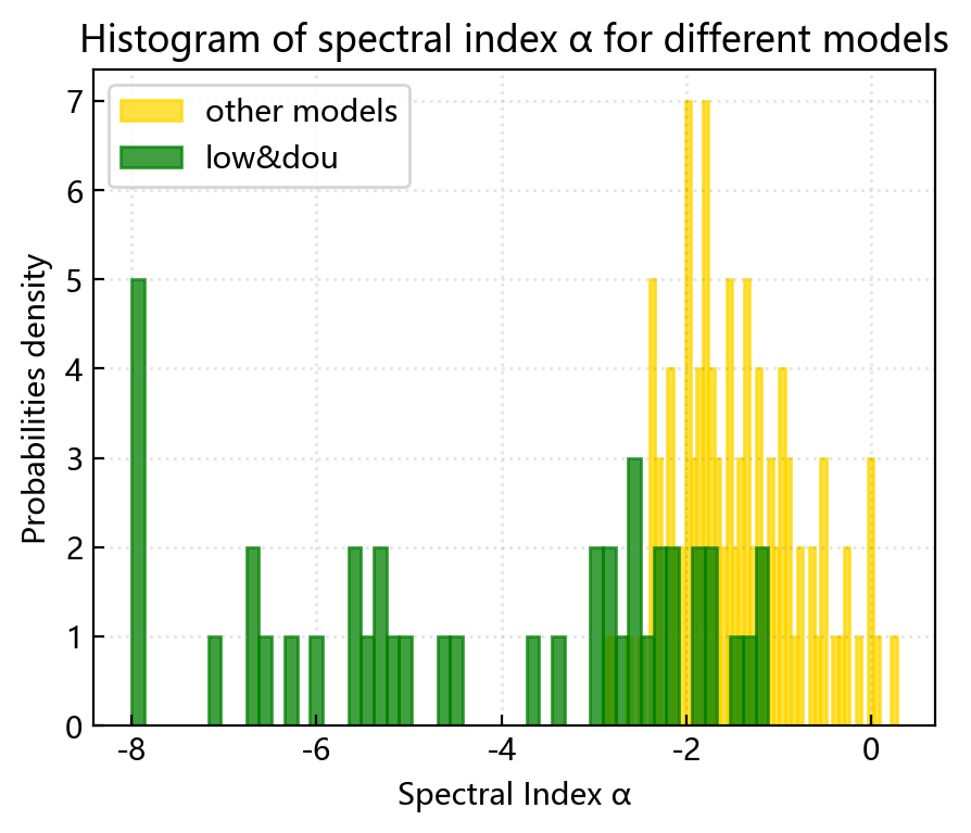
Figure 17: Histogram of the spectral indices $\alpha$ differenr models. The models are categorized into two groups: the low-frequency turnover and the double-turn-over model, and the remaining models fall into the other category.

Table 7: The spectral indices within the same frequency range, bold are those with extremely steep spectral index values.

PSRJ1	$\alpha$	$\alpha$_err	Freq. range (MHz)	Model2
J0452-1759	-0.34	0.07	102.5-4850	bro
J0621+1002*	-6.61	0.12	102.5-4850	low
J0944-1354	-1.82	0.08	102.5-4850	sim
J2337+6151	-1.32	0.11	102.5-4850	sim
J1711-1509	-1.73	0.09	102.5-4850	sim
J1623-0908	-1.73	0.11	102.5-4850	sim
J1916+0951	-1.86	0.06	102.5-4850	sim
J1823+0550	-1.76	0.08	102.5-4850	sim
J0601-0527	-1.77	0.10	102.5-4850	low
J0653+8051	-1.57	0.10	102.5-4850	sim
J1748-1300	-1.87	0.13	102.5-4850	sim
J0040+5716	-0.96	0.51	102.5-4850	bro
J1834-0426	-0.93	0.06	102.5-4850	high
J0758-1528	-1.44	0.08	102.5-4850	sim
J2149+6329	0.06	0.19	102.5-4850	bro
J1910+0358	-1.52	0.09	102.5-4850	sim
J0629+2415	-1.38	0.08	102.5-4850	sim
J2150+5247	-0.74	0.13	102.5-4850	high
J1913-0440	-2.24	0.22	102.5-4850	low
J0406+6138	-5.26	0.07	102.5-4850	low
J1926+0431	-1.19	0.21	102.5-4850	high
J2055+3630	-0.65	0.35	102.5-4850	bro
J1913+1400	-1.53	0.08	102.5-4850	sim
J1754+5201	-0.11	0.22	102.5-4850	high
J2002+4050	-8.00	1.34	102.5-4850	low
J2002+3217	-1.10	0.08	102.5-4850	sim
J1915+1009	-1.94	0.09	102.5-4850	sim
J2013+3845	-0.85	0.08	102.5-4850	high
J1857+0212	-1.29	0.14	102.5-4850	sim
J1257-1027	-1.47	0.08	102.5-4850	sim
J1116-4122	-1.39	0.07	147.5-3100	high
J1045-4509*	-1.24	0.04	147.5-3100	high
J0907-5157	-1.21	0.11	147.5-3100	low
J0959-4809	-1.59	0.09	147.5-3100	sim
J0855-3331	-2.61	0.67	147.5-3100	low
J0846-3533	-2.32	0.24	147.5-3100	low
J1751-4657	-2.78	0.18	147.5-3100	low
J1823-3106	-1.58	0.06	147.5-3100	sim
J1034-3224	-1.19	0.07	147.5-3100	sim
J0857-4424	-2.08	0.05	147.5-3100	sim
J1722-3207	-2.50	0.36	147.5-3100	low
J1801-2920	-2.15	0.45	147.5-3100	low
J1604-4909	-0.93	0.16	147.5-3100	bro
J1743-3150	-3.00	0.20	147.5-3100	low
J1613-4714	-1.70	0.11	147.5-3100	sim
J1801-2451	-0.28	0.15	147.5-3100	high
J1614-5048	-2.00	0.06	147.5-3100	sim
J1836-1008	-6.69	0.05	147.5-3100	low
J1824-2452A	-2.29	0.02	147.5-3100	sim
J1633-5015	-1.04	0.10	147.5-3100	bro
J1717-3425	-2.43	0.24	147.5-3100	low
J1559-4438	-5.16	0.01	147.5-5124	low
J1651-4246	-2.16	0.01	147.5-5124	bro
J1703-3241	-1.34	0.07	147.5-5124	high
J0856-6137	-2.20	0.08	151.5-3100	sim
J0840-5332	-3.02	2.18	151.5-3100	low
J1001-5507	-0.51	0.52	151.5-3100	bro
J2053-7200	-1.16	0.19	151.5-3100	high
J1121-5444	-1.74	0.10	151.5-3100	high
J0942-5657	-2.15	0.11	151.5-3100	sim
J0924-5302	-1.98	0.07	151.5-3100	sim
J0942-5552	-4.68	0.03	151.5-3100	low
J0905-5127	-1.84	0.09	151.5-3100	sim
J1057-5226	-2.53	0.46	151.5-3100	low
J0953+0755	-1.36	0.02	20-22700	dou
J0814+7429	-1.81	0.05	20-22700	low
J1239+2453	-8.00	5.10	20-22700	dou
J0826+2637	-1.48	0.03	20-22700	low
J0837+0610	-6.01	0.04	20-4850	low
J1840+5640	-1.11	0.12	20-4850	dou
J0056+4756	-0.89	0.14	20-4850	high
J1532+2745	-8.00	6.88	25-1420	dou
J1635+2418	-5.40	0.26	25-1420	low
J0934-5249	-2.39	0.14	300-3100	sim
J1739-3023	0.00	0.03	300-3100	high
J1845-0743	-7.13	0.04	300-3100	low
J1841-0425	0.00	0.09	300-3100	high
J1741-3016	-6.32	0.06	300-3100	dou
J1941-2602	-4.54	0.80	350-3100	low
J0818-3232	-2.80	1.20	350-3100	low
J1831-0823	-2.14	0.31	350-3100	low
J1722-3712	-1.79	0.13	350-3100	sim
J1844-0433	-1.78	0.09	350-3100	sim
J0820-3826	-1.77	0.09	350-3100	sim
J2124-3358*	-1.68	0.10	350-3100	low
J1741-3927	-1.28	0.10	350-3100	sim
J1932-3655	-1.23	0.20	350-3100	sim
J1904+0004	-1.12	0.14	350-3100	sim
J1909-3744*	-1.04	0.09	350-3100	sim
J1759-3107	-0.94	0.19	350-3100	high
J1738-3211	-0.88	0.18	350-3100	sim
J1700-3312	-0.78	0.18	350-3100	high
J1708-3426	-0.55	0.84	350-3100	bro
J1817-3618	-0.55	0.16	350-3100	high
J1817-3837	-0.54	0.15	350-3100	high
J0656-2228	-0.36	0.24	350-3100	sim
J1901-0906	-0.26	0.23	350-3100	high
J1727-2739	0.28	0.65	350-3100	bro
J1635-5954	-5.34	0.70	400-3100	low
J1806-1154	-3.70	1.28	400-3100	low
J1017-5621	-2.64	0.27	400-3100	low
J1305-6455	-2.35	0.38	400-3100	sim
J1157-6224	-2.35	0.21	400-3100	sim
J1639-4604	-2.34	0.26	400-3100	sim
J1326-6408	-2.33	0.15	400-3100	sim
J1717-4054	-2.28	0.43	400-3100	sim
J1046-5813	-2.12	0.17	400-3100	sim
J1615-5537	-2.08	0.30	400-3100	sim
J1123-6259	-2.06	0.11	400-3100	sim
J1112-6613	-2.00	0.14	400-3100	sim
J1711-5350	-1.99	0.25	400-3100	sim
J1401-6357	-1.96	0.19	400-3100	sim
J1600-5751	-1.96	0.12	400-3100	sim
J1513-5908	-1.93	0.19	400-3100	low
J1651-5222	-1.90	0.29	400-3100	sim
J1312-5516	-1.85	0.20	400-3100	sim
J1012-5857	-1.76	0.09	400-3100	sim
J1810-5338	-1.66	0.29	400-3100	sim
J0536-7543	-1.66	0.21	400-3100	sim
J1016-5345	-1.64	0.25	400-3100	sim
J1637-4553	-1.45	0.13	400-3100	sim
J1646-6831	-1.43	0.33	400-3100	sim
J1259-6741	-1.35	0.22	400-3100	sim
J0711-6830*	-1.33	0.07	400-3100	sim
J0745-5353	-1.15	0.20	400-3100	high
J1326-6700	-1.07	0.22	400-3100	sim
J1047-6709	-0.62	0.22	400-3100	sim
J2129-5721*	-5.05	3.09	436-3100	low
J1603-7202*	-3.41	0.95	436-3100	low
J1210-5559	-2.79	0.22	436-3100	sim
J1848-1414	-2.34	0.30	436-3100	sim
J1549-4848	-1.99	0.24	436-3100	sim
J1253-5820	-1.53	0.29	436-3100	sim
J1822-4209	-1.51	0.45	436-3100	sim
J0024-7204C*	-8.00	5.15	436-3968	low
J0024-7204D*	-5.63	0.08	436-3968	dou
J1844-0244	-8.00	4.27	606-1606	low
J1826-1131	-2.50	0.15	606-1606	sim
J1845-0434	0.00	0.62	606-1606	high
J1918+1444	-6.71	2.42	606-4850	low
J1824-1118	-2.20	0.11	606-4850	sim
J1820-1346	-1.90	0.18	606-4850	sim
J1901+0716	-1.81	0.13	606-4850	sim
J1808-2057	-0.97	0.19	606-4850	high
J0218+4232*	-5.60	0.11	74-1400	low
J1959+2048*	-2.91	0.07	74-1400	sim
J1843-1113*	-2.64	0.05	74-1400	sim

• The asterisk (*) represents MSPs.

• Here, abbreviations are used for the names of the models, and the names after the abbreviations are indicated in parentheses: broken power law (bro), double turn-over spectrum (dou), and low-frequencies turn-over (low).

4.2 Spectral index correlations

The spectral index of pulsars serves as a characterization of how the flux density evolves with frequency, making it a prominent feature. Additionally, pulsars exhibit characteristic parameters that represent their unique properties. As a result, it is crucial to examine the correlation between spectral index and characteristic parameters of pulsars. The correlation between the spectral index, age, and period of $343$ pulsars was investigated by Lorimer et al. (1995). It was found that the spectral indices of millisecond pulsars exhibit a stronger correlation with the period $(r=+0.51)$ in comparison to normal pulsars. Although the correlation for characteristic age was weak for normal pulsars $(r=-0.19)$ and overall $(r=-0.22)$, they suggested that the characteristic age significantly impacts the spectral index more than the period: young pulsars have predominantly flatter spectra (typically -1) compared to older pulsars for which the corresponding value is 2.

Han et al. (2016) observed a strong correlation between the spectral index and the spin-down luminosity ($r=0.32$) . The results of Han et al. (2016) were supported by Jankowski et al. (2018), who found that, among the $276$ pulsars they studied, the strongest correlation was between the spectral index and the spin-down luminosity ($r=0.44$). Similarly, Zhao et al. (2019) calculated the Spearman correlation coefficients between characteristic parameters in a subset of pulsars ($19$ with simple power-law spectra, and $4$ with broken power-law spectra) and reported a strong correlation between the spectral index and the spin-down luminosity ($r=0.62$). No correlation coefficient exceeded $0.5$ was found in their studies among other parameters.

Our research reveals no strong correlation between the spectral index and the characteristic parameters of both millisecond (see in Figure 16) and normal pulsars (see in Figure 15) when the model was not specified. However, when imposing restrictions and separately analyzing the correlation between the characteristic parameters of normal and millisecond pulsars under different models, significant diversity in the results emerged.

In comparison to normal pulsars (see Table 3), the correlation between the spectral index and specific characteristic parameters of millisecond pulsars is stronger (see Table 4). Specifically, in the case of a simple power-law spectrum, the pulsar distance (Dist) exhibits the strongest correlation with the spectral index ($r=-0.44$), while in the low-frequency turn-over model, the strength of the magnetic field at light cylinder ($B_{\rm{\text{LC}}}$) exhibits the strongest correlation with the spectral index ($r=-0.68$). This phenomenon is likely associated with the size of our sample. Despite having a relatively large sample size compared to previous studies, the number of detected pulsars remains limited. Thus, a strong correlation between the spectral index and certain characteristic parameters is anticipated. Consistent with our previous studies, both millisecond pulsars and normal pulsars exhibit a more pronounced correlation between the spectral index and certain characteristic parameters when the sample size is restricted. Nevertheless, additional sample data is required to validate this assertion.

4.3 Deviations from a simple power-law spectrum

Table 8 presents our data set, covering a frequency range from $30$ MHz to $150$ GHz, that adequately captures the major frequency spectrum. To identify pulsars effectively, we require strict low-frequency and high-frequency coverage criteria. We consider pulsars as having a good low-frequency coverage when they have at least two data points below $600$ MHz. Similarly, pulsars with a good high-frequency coverage have at least one data point above $4$ GHz, as proposed by Jankowski et al. (2018).

Table 8: Fraction of pulsar spectra that can best be characterized by the given spectral model. The first row provides total number of pulsars along with the total number and the second row gives the percentage (out of 886) for each model. The total number and percentage of pulsars with good low-frequency coverage (510) and high-frequency coverage (170) out of the total are presented in the next two columns. The remaining rows indicate the number and percentage (in the third column) of pulsars in the current model (first column) as a proportion of the total, as well as the percentage within the subset of pulsars with good low-frequency coverage (fifth column) and high-frequency coverage (seventh column).

Set	pulsars	percent	low-frequency1 coverage	percent	high-frequency2 coverage	percent
Total	886	-	510	57.56	170	19.19
Simple power law	607	68.51	295	57.84	53	31.18
Double-turn-over spectrum	23	2.60	20	3.92	13	7.65
Broken power law	54	6.09	50	9.80	31	18.24
low-frequency turn-over	95	10.72	69	13.53	48	28.24
high-frequency cut-off	107	12.08	76	14.90	25	14.71

• at least two data points below 600 MHz for pulsars

• at least one data point above 4 GHz

Our study achieved a good high-frequency coverage of 19.19$\%$ and a good low-frequency coverage of 57.56$\%$. We observed that some models’ correlation coefficients changed significantly when a good low-frequency coverage was present, while the overall model ranking remaining the same. The Simple Power Law model correlation coefficient decreased from 68.51$\%$ to 57.56$\%$ (see Table 8), while the remaining four models had an increment in percentage between 1.5$\%$ to 3.8$\%$, indicating a shift in the correlation coefficients of spectral models. A good low-frequency coverage produced deviations from the simple power law spectral model.

With a good high-frequency coverage, we observed considerable changes that impacted the Simple Power Law model prominently. Its correlation coefficient decreased to 31.18$\%$, almost half of the original correlation coefficient. However, the low-frequency turn-over model’s correlation coefficient increased to 28.24$\%$, almost doubling the original value, which almost equals the correlation coefficient of the top-ranked Simple Power Law model. The other three models exhibit variable increases in correlation coefficient, with the high-frequency cut-off Inversion model’s minimal increase is 2.8$\%$. We conclude that deviations from the simple power law spectral model are more pronounced with a good high-frequency coverage.

We observed significant changes in the spectral index with respect to the frequency coverage in Table 9. Firstly, we excluded the broken power law from our study, because it has two distinct spectral indices before and after the turn-over. In cases where there is adequate low frequency coverage ($-1.80\pm 1.30$) and high frequency coverage ($-1.94\pm 1.73$), the mean spectral index ($-1.77\pm 1.31$) remains close to the standard spectral index ($-1.8$) (Maron et al., 2000). If there is good coverage at both low and high frequencies, the spectral index becomes significantly steeper ($-2.01\pm 1.16$). Conversely, when there is no good coverage of both low and high frequencies, the spectral index value is the highest ($-1.73\pm 1.17$).

When considering the impact of frequency coverage, we define a pulsar as having good low-frequency coverage when it has at least two data points below 600 MHz, and good high-frequency coverage when it has at least one data point exceeding 4 GHz. It was observed that the proportion of pulsars conforming to a simple power-law model was 57.84% in the presence of good low frequency coverage, while this percentage dropped to 31.18% in the case of good high frequency coverage. This suggests that pulsars are more inclined to diverge from the simple power-law model as they are observed at higher frequencies. Consequently, a focused analysis was performed on pulsars with frequencies ranging between 600 MHz and 4 GHz, which exhibit inadequate coverage in both low and high frequencies. Among the selected 313 pulsars, the proportion of single power-law models has reached 91.37%. It is posited that with an expanded frequency coverage, the correspondence between the flux density and the frequency may deviate from a simple power-law model. Additionally, when studying the spectral index under different frequency coverage, the spectrum of the pulsar becomes steeper in a wider frequency range (below 600 MHz and above 4 GHz). Of course, there are only 92 objects in our data set that meet this condition, which is far short of a definitive conclusion. For both cases mentioned above, in the future, we need to observe more pulsars at lower and higher frequencies.

Table 9: The spectrum under different frequency coverage. Low-frequency coverage and high-frequency coverage are described in Table 8. Good-frequency coverage means simultaneously having good high-frequency and low-frequency coverage. None-frequency coverage means simultaneously lacking good high-frequency and low-frequency coverage. Total coverage means the spectral index in all models that do not include a broken power law.

Set	mean
low-frequency coverage	$-1.80\pm-1.30$
high-frequency coverage	$-1.94\pm-1.73$
good-frequency coverage	$-2.01\pm-1.56$
none-frequency coverage	$-1.73\pm-1.17$
total coverage	$-1.77\pm-1.31$

4.4 Implications of Spectral Turn-over and Indexes for Physical Models of Pulsar Magnetospheres

The cutoffs at higher frequencies and turn-overs at lower frequencies seen in the spectra of pulsars are inherent characteristic of the physical conditions prevailing inside their magnetospheres. There is considerable consensus that the radio emission of pulsars originates from radiation of the charged particle bunches accelerated along the curved magnetic field lines (Sturrock, 1971; Ruderman & Sutherland, 1975; Philippov & Kramer, 2022). The pulsar magnetospheres are thought to be a tenuous weakly turbulent electron-positron plasma within which various nonlinear processes associated with instabilities and resonances operate under strong magnetic fields to produce electromagnetic waves. Machabeli & Gogoberidze (2005) have shown that scattering of the longitudinal Langmiur plasma waves by the drift of charged particles in the electric field generates a spectrum with index $-1.5$, which is in qualitative agreement with what found from fitting to the pulsar spectra with a simple power-law: $\alpha=-1.57\pm 0.32$ for normal pulsars and $\alpha=-1.89\pm 0.21$ for millisecond pulsars. Refraction of the electromagnetic waves is another key ingredient modifying and re-shaping the formed pulsar spectrum as it is frequency depended (Petrova, 2002). The kinetic energy of the magnetospheric plasma particles acquired during the process of acceleration along the curved magnetic field lines is comparable to the observed brightness temperatures of pulsars and therefore self-absorption of the emitted curvature radiation severely limits the formed spectra. Ochelkov & Usov (1984) suggested that both the breaks and the low frequency turn-overs in the spectra observed from the pulsars arise from the self-absorption of the curvature radiation by emitting bunches themselves. This mechanism naturally accounts for the exponential-like shape of the turn-over. The reason of the appearance of two characteristic frequencies in the spectrum is due to the non-uniformity and anisotropy of the radiation source. These break ($\nu_{\rm b}$) and turn-over ($\nu_{\rm peak}$) frequencies are given by

$$\nu_{\rm b}=\left[\frac{3}{4}\left(\frac{2}{3}\right)^{2/3}\frac{(k-2)e^{2}\theta^{2(k-2)}_{\rm p}\dot{N}}{m_{\rm e}cR^{2}\Gamma}\left(\frac{8}{9}\frac{R}{c\Gamma^{3}}\right)^{-k}\right]^{1/(2+k)},$$ (6)

and

$$\nu_{\rm peak}=\nu_{\rm b}\theta^{[16/3(2+k)]}_{\rm p},$$ (7)

respectively. Here, $k$ is a constant, $e$ and $m_{\rm e}$ are the charge and the mass of electron, $\dot{N}$ is the number of particles ejected from the pulsar per unit time, $c$ is the speed of light, $\Gamma$ is the Lorentz factor, $R$ is the radius of the neutron star and $\theta_{\rm p}=(R\Omega/c)$ is the angular radius of the polar cap with $\Omega=2\pi/P$ being the pulsar’s angular rotation velocity. Their model predicts a spectrum with $\propto\nu^{-4(k-2)/(6+k)}$ before the break and with a much steeper slope $\propto\nu^{-(k-2)}$ after the break. The results presented in Sections 3.1.2 and 3.2.2 agree well with $k=4$ and $k=5$, respectively (see table 1 in Ochelkov & Usov (1984)). The flattening of the pulsar spectra can be understood in terms of the geometry of the hollow-cone model (Kuzmin & Solovev, 1986), as shrinking of the hollow cone width with increasing frequency causes steepening of the emergent radiation. According to Kontorovich & Flanchik (2013a), the high frequency cutoff of the pulsar spectra is a consequence of acceleration of the electrons to the speed of light in the huge electrostatic potential present above the polar cap. In contrast to the conventional models (Sturrock, 1971; Ruderman & Sutherland, 1975), their theory assumes a zero potential at the neutron star surface, a linear increasing electrostatic field just above the polar cap which passes through a maximum slowly and then experiences rapid decline when electrons approach to the relativistic limit. This results in a flat spectrum radiated by a large number of electrons accelerated in the corresponding potential across the polar gap. That theoretical model predicts a cutoff frequency

$$\nu_{\rm c}\approx\sqrt{2\left(\frac{B}{2\times 10^{12}\,\mbox{G}}\right)\left(\frac{1\,\mbox{s}}{P}\right)}\,\mbox{GHz},$$ (8)

while empirical relation found earlier by Malov & Malofeev (1981) states that the cutoff position in the spectrum is

$$\nu_{\rm c}\approx 1.4\left(\frac{1\,\mbox{s}}{P}\right)^{0.46\pm 0.18}\,\mbox{GHz}.$$ (9)

Also their model is capable of explaining a low frequency turn-over occurring naturally at $\nu_{\rm peak}\approx 0.1\nu_{\rm c}$ (Kontorovich & Flanchik, 2013b). Equation (8) may, in principle, account for the rarity of pulsars showing cutoff behaviour in their spectra (see Table 2), since for most of them the emission region shifts to a thin and narrow layer. The absence of a low frequency turn-over in the spectrum, especially in the case of millisecond pulsars, can be attributed to deviation of the magnetic field configuration from a dipolar structure or to compactness of the emission region (Kuzmin & Losovsky, 2001). In addition to these, other geometrical factors like curvature radius of the magnetospheric field lines, altitude of the emission region above the polar cap and orientation of the magnetic dipolar axis with respect to the rotational axis affect the spectral shape as well and may lead to high energy cutoff observed from a given pulsar (Malov & Malofeev, 1991). Another possibility applicable for spectral turn-over at high frequencies seen from GPS pulsars is the free-free absorption of the pulsar emission by the interstellar matter with HII regions, pulsar wind nebulae and supernova remnants being the primary sources (Kijak et al., 2017). For example, PSR J1056–6258 is known to be surrounded by an ionized hydrogen region (Koribalski et al., 1995). Another case supporting the view that environment may cause inversion of the spectra of pulsars at high frequencies is PSR B1259–63 which orbits around a Be star. It is observed that the pulsar’s spectrum evolves regularly as it approaches to the companion star during binary motion (Kijak et al., 2011). Model fitting to the temporal evolution of the pulsar spectra with the free-free absorption may in principle enable one to estimate the electron density and the size of the absorbing medium. For instance, by using this method Basu et al. (2016) constrained the physical properties of the medium enclosures PSR B1800–21. By examining 33 GPS pulsars, Li et al. (2023) arrived at the conclusion that their spectral indices obey a bimodal distribution. They also found a strong positive relation between periods $P$ and DMs of GPS pulsars. This suggests that at least some of the GPS pulsars may be evolved through interaction with a fallback disk for which there exists interplay between the slow-down torque and the amount of the dispersive matter settled down around the neutron star after the supernova explosion (Alpar, 2001; Menou et al., 2001).

5 Conclusions

In our work, we combined an open-source database developed by Swainston et al. (2022) to determine flux density values for a total of 941 pulsars. The total covered frequency range was from $30$ MHz to $150$ GHz, and each pulsar had at least $4$ different flux density values. After excluding some pulsars that cannot be fitted, we determined the spectral values of $886$ pulsars. Subsequently, we applied five distinct spectral models to fit the data. Our results can be summarized as follows:

• The spectral indexes of our sample is normally distributed, with a weighted mean is $-1.61\pm 0.32$.

• Overall, $68.51$% of the pulsars fit within the range of the simple power law model, while $31.5$% deviate from it, showing other characteristics. Among them, $12.08$% showed high-frequency cut-off, and $10.72$% showed low-frequency turn-over characteristics.

• At both high and low frequencies, pulsars tend to deviate more from a simple power-law spectrum and have a steeper spectral index.

• Compared to normal pulsars, millisecond pulsars exhibit stronger correlations with characteristic parameters. It is noteworthy to keep in mind that this research examined only a total of 86 millisecond pulsars.

• In our statistical work, 33 GPS pulsars have been identified. Of these, 11 had been mentioned in previous literature, and 22 were identified for the first time.

Table A1: Pulsars that have broken power-law spectra, where $\nu_{br}$ is the frequency of the spectral break, $\alpha_{1}$ and $\alpha_{2}$ the spectral index before and after the break for a given frequency range. They are followed by corresponding errors. We also mark the MSPs with*.

PSRJ	$\alpha_{1}$	$\alpha_{1}$_err	$\alpha_{2}$	$\alpha_{2}$_err	$\nu_{br}$(MHz)	$\nu_{br}$_err(MHz)	Freq.range(MHz)
J0040+5716	-0.96	0.51	-1.74	0.08	408	0.2	102.5-4850
J0147+5922	-1.52	0.13	-0.52	0.13	760.9	189.4	102.5-4920
J0437-4715*	-0.92	0.01	-1.71	0.15	1400.1	489.3	76-17000
J0452-1759	-0.34	0.07	-2.13	0.11	699.9	64.5	102.5-4850
J0543+2329	-0.21	0.15	-1.53	0.12	814.6	90	102.5-10550
J0612+3721	-0.03	0.45	-2.05	0.17	447.5	70.9	59.66-4850
J0742-2822	-1.15	0.09	-1.57	0.12	1582.2	669.1	102.5-10550
J0820-4114	-0.67	0.23	-2.32	0.42	500.7	151	76-3100
J1001-5507	-0.51	0.52	-2.58	0.28	567.6	190.3	151.5-3100
J1024-0719*	-1.42	0.09	-0.64	0.19	1400	0.6	102-4850
J1059-5742	-1.06	0.44	-2.64	0.35	684.1	264.2	154.24-3100
J1141-6545	3.00	2.14	-2.57	0.26	254.5	18	154.24-3100
J1146-6030	-0.37	0.23	-1.62	0.24	600	22.4	154.24-3100
J1224-6407	-0.80	0.10	-1.54	0.15	843	0.5	154.24-3100
J1300+1240	3.00	7.17	-2.53	0.14	105.7	6.7	50-1400
J1326-5859	0.94	2.31	-1.88	0.25	647.1	201.7	400-8356
J1453+1902*	-0.98	0.22	-2.68	1.32	480	346.9	149-2100
J1455-3330*	-1.57	0.36	-2.83	0.39	660	3	154.24-1520
J1518+4904	-0.19	0.66	-2.44	0.32	1156.6	297.3	102-4850
J1600-5044	-0.63	0.08	-2.05	0.08	728	0.2	147.5-8356
J1604-4909	-0.93	0.16	-2.47	0.42	950	0.3	147.5-3100
J1633-5015	-1.04	0.10	-2.51	0.24	843	0.4	147.5-3100
J1643-1224*	-1.79	0.04	-1.38	0.09	1284	0.2	147.5-4850
J1644-4559	2.50	0.10	-2.07	0.00	729.9	3	147.5-17000
J1651-4246	-2.16	0.01	-2.47	0.12	1315.9	58.3	147.5-5124
J1705-1906	-1.11	0.11	-0.30	0.32	4850	17.1	102.5-8600
J1708-3426	-0.55	0.84	-2.99	0.31	816	130.4	350-3100
J1713+0747*	-0.13	0.07	-2.55	0.16	2030	81	102-4850
J1727-2739	0.28	0.65	-2.07	0.19	939.9	231.6	350-3100
J1739-3131	-0.61	0.06	-4.78	0.81	1369	0.1	300-1606
J1803-2137	1.70	0.11	-0.59	0.03	835.2	33.5	300-8600
J1807-0847	-0.03	0.27	-1.62	0.12	843	1.4	102.5-8600
J1809-1917	0.96	0.26	-1.45	0.37	1908.2	231.1	325-6591
J1813+4013	-0.97	0.16	-2.91	0.60	862.5	228.8	59.67-2600
J1816+4510*	0.94	2.03	-2.54	0.38	142.5	0.4	74-820
J1823-1115	0.21	0.19	-1.56	0.13	628.4	56.1	300-4850
J1833-0338	-0.98	0.10	-3.01	0.13	475.5	24.3	102.5-3100
J1841+0912	-0.97	1.13	-1.95	0.09	296.9	388.7	59.73-4850
J1844+1454	-1.27	0.80	-4.40	0.49	102.5	0.6	49.8-1420
J1849-0636	2.23	2.18	-2.32	0.09	157.9	7.5	102.5-3100
J1857+0943*	-1.50	0.07	-0.01	0.11	1405.1	12.6	102-4850
J1907+4002	-0.32	0.24	-2.07	0.12	480.4	72.3	100-4850
J1909+1102	1.07	1.94	-2.54	0.10	178.7	20.6	102.5-4920
J1918-0642*	-1.59	0.06	-8.00	0.40	1284	0.2	149-1400
J1935+1616	-0.45	0.06	-3.32	0.66	2291.9	648.1	135.25-22700
J1939+2134	-1.51	0.02	-2.93	0.21	1805.6	227.8	74-4850
J2022+2854	1.03	0.61	-1.29	0.10	100.2	21.6	24.75-22700
J2055+3630	-0.65	0.35	-1.97	0.08	454.6	30.7	102.5-4850
J2149+6329	0.06	0.19	-2.10	0.13	472.3	23.8	102.5-4850
J2155-3118	-1.27	0.23	-2.60	0.22	534.7	129.5	147.5-1408
J2229+6205	-0.28	0.79	-2.30	0.16	235.6	59.8	102.5-1410
J2308+5547	-0.81	0.72	-8.00	2.48	236.1	25.8	59.66-1420
J2317+2149	0.47	0.38	-2.05	0.09	198.1	21.4	25-4850
J2321+6024	0.05	0.26	-2.97	0.41	1161.7	66.9	102.5-22700

Table A2: Pulsars that have power-law spectra with a low-frequency turn-over, where $\nu_{p}$ is the peak/turn-over frequency, $\alpha$ is the spectral index for a given frequency range, and $\beta$ is the free fit parameter that determines the smoothness of the turn-over. They are followed by corresponding errors. We also mark the MSPs with*.

PSRJ	$\alpha$	$\alpha$_err	$\beta$	$\beta$_err	$\nu_{p}$(MHz)	$\nu_{p}$_err(MHz)	Freq.range(MHz)
J0024-7204C*	-8.00	5.15	0.38	0.00	600.4	9	436-3968
J0024-7204J*	-8.00	0.34	2.10	0.08	607.8	4.5	768-3968
J0151-0635	-0.80	0.18	2.10	1.94	71	10.6	25-1408
J0218+4232*	-5.60	0.11	2.10	0.33	174.2	0.7	74-1400
J0304+1932	-7.93	0.10	0.12	0.00	184.1	11.6	24.75-4850
J0323+3944	-3.25	1.36	0.63	0.44	80.8	15.5	25-1408
J0406+6138	-5.26	0.07	0.12	0.00	61.1	5.7	102.5-4850
J0601-0527	-1.77	0.10	1.87	1.83	139.2	47.4	102.5-4850
J0613-0200*	-2.46	0.21	1.41	0.41	466.6	46.3	102-3100
J0614+2229	-2.20	0.09	2.10	0.30	216.7	9.4	85-4850
J0621+1002*	-6.61	0.12	0.14	0.00	114.8	7.5	102.5-4850
J0700+6418	-2.60	0.41	1.49	0.49	78.1	5.8	49.8-1408
J0738-4042	-2.76	0.02	0.60	0.00	397.1	3.3	107-17000
J0809-4753	-2.62	0.23	1.46	0.40	127.2	6.8	76-3100
J0814+7429	-1.81	0.05	2.01	1.42	46.8	0.6	20-22700
J0818-3232	-2.80	1.20	1.59	1.69	525	38.6	350-3100
J0820-1350	-3.62	0.66	0.29	0.05	57.8	13.8	58.6-4850
J0826+2637	-1.48	0.03	2.10	0.24	45.7	3.2	20-22700
J0828-3417	-5.06	0.53	1.22	0.27	147.7	2.5	76-1400
J0835-4510	-2.06	0.18	0.53	0.14	99.2	10.1	76-343500
J0837+0610	-6.01	0.04	0.23	0.00	60.7	3.8	20-4850
J0837-4135	-2.43	0.20	1.07	0.21	272.4	11.2	147.5-8600
J0840-5332	-3.02	2.18	0.76	1.26	153.1	112.1	151.5-3100
J0846-3533	-2.32	0.24	2.10	1.51	498.1	28.6	147.5-3100
J0855-3331	-2.61	0.67	0.68	0.52	43.5	4.8	147.5-3100
J0907-5157	-1.21	0.11	2.10	1.99	156.8	19	147.5-3100
J0908-1739	-1.45	0.07	2.10	1.33	84.2	1.4	49.8-4850
J0908-4913	-1.98	0.41	1.22	0.77	603.5	42.3	400-17000
J0942-5552	-4.68	0.03	0.47	0.00	305.1	6.5	151.5-3100
J0943+1631	-1.80	0.56	1.22	1.47	71.1	22.5	25-3100
J1017-5621	-2.64	0.27	2.10	2.00	434.9	108.5	400-3100
J1056-6258	-1.47	0.23	2.10	1.38	580.9	96	400-8356
J1057-5226	-2.53	0.46	2.10	1.66	186.4	27.2	151.5-3100
J1243-6423	-5.71	0.57	2.10	2.00	562.6	44.5	408-8356
J1327-6222	-2.17	0.26	1.71	1.11	216.2	24.5	151.5-6591
J1359-6038	-2.31	0.14	1.88	1.88	179.6	36.4	151.5-8356
J1430-6623	-1.92	0.20	2.10	1.30	238.7	13.8	151.5-8356
J1453-6413	-2.64	0.17	2.10	0.15	192.9	8.8	102-8356
J1513-5908	-1.93	0.19	2.10	1.37	611.6	65.6	400-3100
J1524-5706	-2.43	0.46	2.10	1.43	1189.4	65.2	728-3100
J1559-4438	-5.16	0.01	0.34	0.00	403.8	2.7	147.5-5124
J1600-3053*	-7.57	0.05	0.22	0.00	847	18.7	350-4820
J1603-7202*	-3.41	0.95	1.65	1.49	594.2	28	436-3100
J1614+0737	-2.09	0.29	1.38	1.50	52.3	7.8	25-4850
J1623-2631	-7.97	0.20	0.31	0.01	395.2	21.8	106.5-2695
J1635+2418	-5.40	0.26	0.30	0.02	73.2	8.5	25-1420
J1635-5954	-5.34	0.70	2.10	1.84	857.2	59.9	400-3100
J1651-5255	-8.00	0.04	0.40	0.00	473.2	15.8	40-3100
J1705-3950	-1.13	0.46	2.10	1.73	1039.4	71.9	610-3100
J1709-4429	-1.43	0.09	2.10	1.41	485.4	55	400-8600
J1717-3425	-2.43	0.24	2.10	1.57	175.6	20.7	147.5-3100
J1722-3207	-2.50	0.36	0.78	0.32	44.8	2.5	147.5-3100
J1731-4744	-2.09	0.08	2.10	0.29	214.7	2.5	133-3100
J1740-3015	-1.14	0.17	2.10	0.32	951.4	146.7	350-17000
J1743-3150	-3.00	0.20	2.10	1.27	476.4	10.4	147.5-3100
J1745-3040	-1.37	0.09	2.10	0.21	1009.9	130.2	350-10550
J1751-3323	-1.40	0.99	1.76	1.72	1006.2	109.3	610-3100
J1751-4657	-2.78	0.18	2.10	1.45	184.5	14.9	147.5-3100
J1753-2501	-2.84	2.04	0.51	0.45	760.8	91.1	300-4850
J1757-2421	-1.81	0.14	2.10	0.17	557.8	10.4	300-6591
J1801-2304	-6.95	0.12	0.15	0.00	261.6	17.3	300-8000
J1801-2920	-2.15	0.45	1.61	1.75	157.9	46.8	147.5-3100
J1806-1154	-3.70	1.28	1.98	1.94	642.3	64.7	400-3100
J1818-1422	-3.13	0.19	1.26	0.08	886.1	54	606-5124
J1820-0427	-2.38	0.04	2.10	0.05	127.2	0.3	102.5-4920
J1822-2256	-3.28	0.24	0.62	0.07	231.3	38.4	350-4850
J1826-1334	-0.78	0.52	1.06	0.57	1220.1	134.6	325-4920
J1830-1059	-8.00	7.98	0.36	0.05	913.1	47.8	606-4920
J1831-0823	-2.14	0.31	2.10	1.07	450.5	40.8	350-3100
J1832-0827	-3.55	0.91	0.84	0.34	573.3	27.5	300-6591
J1833-0827	-4.35	0.99	0.20	0.06	394.8	126.6	300-4920
J1835-1020	-2.78	0.12	0.65	0.02	587.7	31.1	325-4850
J1836-1008	-6.69	0.05	0.26	0.00	209.6	6.6	147.5-3100
J1843-0000	-1.83	0.06	2.10	1.58	472.3	21.1	350-5124
J1843-0459	-3.78	0.52	2.10	1.77	807.4	59.1	728-3100
J1844-0244	-8.00	4.27	0.89	0.35	861.1	45.7	606-1606
J1844-0538	-2.10	0.20	2.10	0.42	1008	57.2	500-4850
J1845-0743	-7.13	0.04	0.31	0.00	804.5	9.1	300-3100
J1852-0635	-0.99	0.03	2.10	0.10	1119	41.1	610-8350
J1905-0056	-4.31	0.09	0.29	0.01	74.4	7.4	102.5-3100
J1909+0254	-2.78	0.27	1.93	1.91	136.6	33.1	102.5-1410
J1913-0440	-2.24	0.22	1.09	0.53	48.3	4.3	102.5-4850
J1918+1444	-6.71	2.42	2.09	1.99	1998.4	1640.8	606-4850
J1941-2602	-4.54	0.80	2.10	0.39	484.6	14.6	350-3100
J1943-1237	-2.22	0.16	2.10	1.77	159.6	17.7	147.5-1408
J2002+4050	-8.00	1.34	0.20	0.00	247.2	9.5	102.5-4850
J2004+3137	-2.70	0.21	2.10	1.42	424.4	26.3	350-4850
J2046-0421	-2.73	1.00	0.99	0.73	193.6	21.7	102.5-3100
J2113+2754	-1.89	0.10	2.10	1.53	42.6	4.9	25-4850
J2124-3358*	-1.68	0.10	2.10	1.28	440.1	48	350-3100
J2129-5721*	-5.05	3.09	1.22	1.55	567.6	65.6	436-3100
J2219+4754	-3.23	0.09	0.50	0.02	41.6	4	35.1-1435
J2305+3100	-1.44	0.06	2.10	1.33	94.5	7.7	49.8-4850
J2313+4253	-1.39	0.12	1.73	1.70	58.9	15.4	25-10550
J2330-2005	-2.05	0.07	2.10	0.44	75.7	0.8	35.1-4920

Table A3: Pulsars that have power-law spectra with a high-frequency cut-off, where $\nu_{\rm c}$ is the cut-off frequency and $\alpha$ is the spectral index for a given frequency range. They are followed by corresponding errors. We also mark the MSPs with*.

PSRJ	$\alpha$	$\alpha$_err	$\nu_{\rm c}$(MHz)	$\nu_{\rm c}$_err(MHz)	Freq.range(MHz)
J0056+4756	-0.89	0.14	5984.60	744.80	20-4850
J0102+6537	0.00	0.49	1944.60	167.00	102.5-1606
J0108+6608	-1.16	0.22	2277.40	725.00	65-1408
J0133-6957	-0.18	0.17	1431.50	5.90	154.24-1400
J0357+5236	-0.60	0.19	2194.30	346.30	102.5-1606
J0450-1248	-1.46	0.12	2376.80	491.10	102.5-1420
J0502+4654	-0.35	0.23	1927.30	193.10	102.5-1420
J0525+1115	-0.88	0.11	1884.90	109.50	61-1420
J0533+0402	0.00	4.93	1525.80	47.50	102.5-1360
J0737-3039A	-1.57	0.06	8136.30	1698.80	99-5000
J0745-5353	-1.15	0.20	5765.20	1538.80	400-3100
J0838-2621	-0.22	0.34	1689.00	114.20	350-1460.04
J0904-7459	-0.83	0.19	4026.00	876.20	154.24-3100
J0921+6254	-0.44	0.21	1731.00	296.10	24.75-1408
J0955-5304	-0.69	0.22	1546.00	40.70	154.24-1440
J1003-4747	-1.20	0.10	5211.10	1205.10	154.24-3100
J1012+5307*	-0.85	0.07	5332.70	245.50	102-4850
J1018-1642	-1.33	0.27	1981.00	422.80	102.5-1420
J1045-4509*	-1.24	0.04	4622.00	158.70	147.5-3100
J1048-5832	-0.45	0.12	19191.80	1070.70	640-17000
J1110-5637	-0.53	0.22	4171.90	684.40	640-3100
J1114-6100	0.00	0.87	4053.30	635.10	640-3100
J1116-4122	-1.39	0.07	3467.50	220.90	147.5-3100
J1121-5444	-1.74	0.10	5562.30	2422.60	151.5-3100
J1136-5525	-0.20	0.15	1774.30	178.00	154.24-1382
J1225-6408	0.00	0.07	1440.00	44.50	400-1440
J1238+2152	0.00	0.16	424.00	20.90	25-400
J1239-6832	-1.31	0.15	4164.10	997.20	154.24-3100
J1302-6350	0.00	0.17	12342.00	4034.60	640-8356
J1313+0931	-0.66	0.16	1507.40	26.30	57-1400
J1320-5359	-1.36	0.10	6880.60	2477.00	154.24-3100
J1355-5153	-1.54	0.12	1761.20	128.20	147.5-1369
J1440-6344	-0.87	0.19	1519.10	46.60	154.24-1400
J1452-6036	0.00	0.19	4515.00	294.80	728-3100
J1507-6640	-1.23	0.36	2185.90	250.70	400-1460.04
J1512-5759	-0.99	0.20	3986.10	327.60	640-3100
J1553-5456	-1.46	0.49	2022.30	236.60	400-1459.32
J1645+1012	-0.33	0.58	452.10	16.70	59.68-430
J1646-4346	-0.81	0.33	5992.80	1059.90	1350-4860
J1652+2651	0.00	0.15	920.10	79.70	102.5-800
J1700-3312	-0.78	0.18	4160.90	866.80	350-3100
J1700-3611	-0.17	0.28	1984.80	198.00	350-1460.04
J1703-1846	-0.99	0.15	1720.00	515.00	102.5-1720
J1703-3241	-1.34	0.07	11407.00	5731.20	147.5-5124
J1707-4053	-1.54	0.31	8063.70	1337.20	147.5-6591
J1709-1640	-0.90	0.04	25259.00	2968.40	49.8-22700
J1720-0212	-0.79	0.16	1551.20	53.80	102.5-1420
J1720-1633	-1.47	0.12	6006.00	587.90	147.5-4850
J1721-3532	-0.47	0.06	21938.70	2340.60	1360-17000
J1723-3659	0.00	0.23	4016.50	252.30	325-3100
J1730-2304*	-1.22	0.09	3334.60	224.90	102-3100
J1733-2228	-0.04	0.91	1597.30	136.10	350-1435
J1735-0724	-0.08	0.30	1567.50	71.80	102.5-1408
J1736-2457	-0.43	0.30	1886.30	105.10	350-1460.04
J1738-2330	-0.45	0.89	1794.80	154.70	350-1460.04
J1739-3023	0.00	0.03	3487.90	112.90	300-3100
J1740+1000	-0.44	0.06	13966.90	1697.30	149-8350
J1741-2733	-0.76	0.17	2153.70	188.10	350-1459.32
J1754+5201	-0.11	0.22	5052.10	114.90	102.5-4850
J1756-2435	-0.35	0.21	3711.50	274.80	606-3100
J1757-2223	0.00	0.04	3913.10	301.70	325-3100
J1759-3107	-0.94	0.19	4326.00	1017.20	350-3100
J1801-0357	-1.15	0.29	1758.80	181.30	102.5-1420
J1801-2451	-0.28	0.15	3516.80	149.10	147.5-3100
J1804-2717*	-0.27	0.50	1500.60	61.40	350-1400
J1807-2715	-1.69	0.37	1959.40	376.00	350-1420
J1808-0813	-1.38	0.19	3999.10	546.20	102.5-3100
J1808-2057	-0.97	0.19	5905.50	440.50	606-4850
J1810+1744*	-0.55	0.29	416.50	13.70	74-400
J1812-1733	-0.92	0.18	4256.80	197.80	728-4000
J1816-1729	-0.27	0.36	2415.60	514.60	147.5-1606
J1816-2650	-0.93	0.28	1952.50	278.70	350-1400
J1817-3618	-0.55	0.16	3373.30	242.00	350-3100
J1817-3837	-0.54	0.15	4497.70	735.10	350-3100
J1825+0004	-1.10	0.30	1729.20	227.60	102.5-1408
J1828-1101	-0.14	0.28	5015.80	150.90	1360-4850
J1829-1751	-0.95	0.06	11601.90	714.00	147.5-10550
J1834-0426	-0.93	0.06	6791.10	572.70	102.5-4850
J1835-0643	-1.08	0.07	5227.50	441.00	147.5-4850
J1837-0653	-1.08	0.30	4413.70	1196.70	102.5-3100
J1841-0425	0.00	0.09	3875.00	182.40	300-3100
J1842-0153	-0.37	0.30	3565.80	232.30	728-3100
J1843-0211	-0.51	0.29	3903.30	412.70	728-3100
J1845-0434	0.00	0.62	2432.00	255.40	606-1606
J1850+0026	-0.78	0.22	2330.70	377.10	350-1459.32
J1850+1335	-0.53	0.37	1694.20	158.90	102.5-1606
J1852+0031	-0.50	0.10	5210.50	80.50	300-4850
J1855-0941	-0.54	0.28	1777.80	88.60	350-1460.04
J1901-0906	-0.26	0.23	3209.40	74.30	350-3100
J1903+0327*	0.00	0.12	5675.10	242.70	74-5000
J1903-0632	-1.74	0.07	3500.70	246.70	102.5-3100
J1909+0007	-1.08	0.19	1740.40	114.90	102.5-1408
J1910-0309	-1.91	0.18	2198.20	574.90	102.5-1420
J1912+2104	-0.13	0.25	1721.80	135.70	149-1615
J1921+1948	-0.94	0.13	1715.50	131.20	147.5-1420
J1926+0431	-1.19	0.21	6965.00	1472.40	102.5-4850
J1946-2913	-0.60	0.34	1530.90	90.10	350-1408
J2007+2722	0.00	0.08	10216.00	950.40	610-9000
J2013+3845	-0.85	0.08	6204.90	394.10	102.5-4850
J2051-0827*	-1.37	0.06	26950.00	18220.90	111-2695
J2053-7200	-1.16	0.19	3411.80	353.90	151.5-3100
J2116+1414	-0.64	0.35	1889.30	282.10	135.25-1420
J2150+5247	-0.74	0.13	6646.20	676.10	102.5-4850
J2157+4017	-0.46	0.06	5013.80	30.80	100-4850
J2212+2933	-0.01	4.28	1591.60	365.30	102.5-1420
J2225+6535	-1.14	0.13	2704.20	746.90	59.7-1606
J2325+6316	0.00	0.23	1740.60	151.40	102.5-1420

Table A4: Double turn-over spectrum (has a low-frequency turn-over and a high-frequency cut-off), where $\alpha$ is the spectral index for a given frequency range, $\beta$ the smoothness of the turn-over, $\nu_{c}$ and $\nu_{p}$ the cut off frequency and the peak/turn-over frequency. They are followed by corresponding errors. We also mark the MSPs with*.

PSRJ	$\alpha$	$\alpha$_err	$\beta$	$\beta$_err	$\nu_{p}(MHz)$	$\nu_{p}$_err(MHz)	$\nu_{c}$(MHz)	$\nu_{c}$_err(MHz)	Freq.range(MHz)
J0024-7204D*	-5.63	0.08	0.21	0.00	689.5	40.6	4225	239.4	436-3968
J0030+0451*	-2.26	0.02	2.10	1.26	55.1	0.2	21000	16672.1	50-2100
J0034-0534*	-4.70	0.29	1.30	0.09	84.1	0.5	16600	14507	50-1660
J0034-0721	-3.44	0.18	0.74	0.05	72.7	2	14350	9435	20-1435
J0141+6009	-1.47	0.07	2.10	1.64	102	9.9	6654.4	590.7	58.6-4850
J0630-2834	-1.86	0.03	2.10	0.14	83.5	0.4	105500	57713.6	35.1-10550
J0946+0951	-5.54	2.19	0.72	0.43	53	2.8	14080	6881.1	20-1408
J0953+0755	-1.36	0.02	2.10	0.30	53.4	2.1	26832.9	641.5	20-22700
J1022+1001*	-1.13	0.26	1.36	1.50	73.3	16.2	8158.3	2184.9	50-4850
J1239+2453	-8.00	5.10	0.41	0.04	71.5	2.9	22700	182092.8	20-22700
J1456-6843	-2.61	0.10	2.10	0.21	259	2.7	83560	74046.4	102-8356
J1532+2745	-8.00	6.88	0.40	0.07	69.4	8.5	1420	8199	25-1420
J1607-0032	-1.93	0.13	1.66	0.24	78.8	3.5	105500	55751.5	25-10550
J1741-3016	-6.32	0.06	0.28	0.00	947.9	26.3	3719.2	203.8	300-3100
J1825-0935	-0.92	0.09	2.10	1.27	54.8	7.1	12061.8	986.2	25-10550
J1825-1446	-3.79	0.08	0.13	0.00	1722.7	223.8	9265.1	969.8	325-8000
J1832-1021	-5.51	0.05	0.37	0.01	2000	1483.6	1674.3	18.8	408-1606
J1840+5640	-1.11	0.12	2.10	1.62	44.9	2.8	6563.7	932.3	20-4850
J1911-1114*	-8.00	7.05	0.21	0.00	139.7	8.8	7757.3	10512.6	102-1660
J1932+1059	-1.06	0.03	1.63	0.34	63.7	6.5	50801.4	5737.5	20-43000
J1955+2908*	-3.31	0.94	1.34	0.77	168.8	17.6	14000	9748.2	147.5-1400
J2048-1616	-1.27	0.04	2.10	2.00	10	57.1	22700	7481.4	102.5-22700
J2145-0750*	-1.89	0.07	1.61	0.19	108.5	5.5	51240	45404	50-5124

Table A5: The pulsars that cannot be accurately fitted by the program. We independently fit each pulsar using the least-squares method, calculate the spectral index $\alpha$ along with its uncertainty $\alpha$_err, and provide the corresponding frequency range.

PSRJ	$\alpha$	$\alpha$_err	Freq.range(MHz)
J1115+5030	-0.86	0.24	20-1435
J1543-0620	-1.11	0.31	25-1435
J1921+2153	-1.52	0.30	20-1420
J1948+3540	-1.48	0.29	102.5-8600
J1955+5059	-0.93	0.23	59.66-4920
J0014+4746	-0.78	0.27	59.14-1435
J0214+5222	-1.38	0.62	50-820
J0332+5434	-1.29	0.11	25-43000
J0459-0210	-2.08	0.22	102.5-1360
J0534+2200	-1.36	0.81	102.5-1435
J0659+1414	-0.84	0.19	85-8600
J0922+0638	-1.40	0.12	20-10550
J1136+1551	-1.34	0.10	20-22700
J1645-0317	-1.61	0.11	49.8-22700
J1741-0840	-1.66	0.51	102.5-4850
J1848-0123	-1.50	0.20	102.5-10550
J1900-2600	-1.61	0.25	147.5-4820
J1903+0135	-1.46	0.51	350-4850
J1922+2110	-1.59	0.66	135.25-1435
J2022+5154	-0.81	0.11	65-43000
J2108+4441	-1.03	0.45	135.25-1435
J2113+4644	-1.44	0.31	102.5-10550
J2354+6155	-0.98	0.27	102.5-10550
J0454+5543	-0.99	0.19	25-10550
J0139+5814	-1.62	0.23	102.5-10550
J0152-1637	-1.51	0.18	35.1-1440
J0157+6212	-0.82	0.56	102.5-1408
J0528+2200	-1.25	0.15	39-22700
J1509+5531	-1.30	0.26	20-4820
J1543+0929	-1.87	0.27	53-4850
J1740+1311	-1.32	0.23	59.65-4850
J1752-2806	-1.83	0.19	61-22700
J1759-2205	-1.65	0.43	147.5-3100
J1824-1945	-1.36	0.29	147.5-3100
J1847-0402	-1.62	0.41	102.5-3100
J1901+0331	-2.04	0.52	102.5-3100
J1902+0556	-1.39	0.52	102.5-3100
J1916+1312	-1.70	0.38	102.5-4850
J1917+1353	-1.67	0.33	102.5-4850
J1919+0021	-1.95	0.88	135.25-1410
J1954+2923	-0.47	0.30	25-4920
J2018+2839	-1.27	0.15	25-22700
J2257+5909	-1.33	0.46	102.5-4820
J2326+6113	-0.91	0.52	102.5-1420

References

- Aloisi et al. (2019) Aloisi, R., Cruz, A., Daniels, L., et al. 2019, The Astrophysical Journal, 875, 19
- Alpar (2001) Alpar, M. A. 2001, ApJ, 554, 1245, doi: 10.1086/321393
- Bailes et al. (1997) Bailes, M., Johnston, S., Bell, J., et al. 1997, The Astrophysical Journal, 481, 386
- Basu et al. (2018) Basu, R., Rożko, K., Kijak, J., & Lewandowski, W. 2018, Monthly Notices of the Royal Astronomical Society, 475, 1469
- Basu et al. (2016) Basu, R., Rożko, K., Lewandowski, W., Kijak, J., & Dembska, M. 2016, MNRAS, 458, 2509, doi: 10.1093/mnras/stw394
- Bhat et al. (2023) Bhat, N., Swainston, N., McSweeney, S., et al. 2023, Publications of the Astronomical Society of Australia, 40, e020
- Biggs & Lyne (1996) Biggs, J., & Lyne, A. 1996, Monthly Notices of the Royal Astronomical Society, 282, 691
- Boyles et al. (2013) Boyles, J., Lynch, R. S., Ransom, S. M., et al. 2013, The Astrophysical Journal, 763, 80
- Brinkman et al. (2018) Brinkman, C., Freire, P. C., Rankin, J., & Stovall, K. 2018, Monthly Notices of the Royal Astronomical Society, 474, 2012
- Camilo & Nice (1995) Camilo, F., & Nice, D. J. 1995, ApJ, 445, 756, doi: 10.1086/175737
- Champion et al. (2005) Champion, D., Lorimer, D., McLaughlin, M., et al. 2005, Monthly Notices of the Royal Astronomical Society, 363, 929
- Champion (2005) Champion, D. J. 2005, Pulsar searching and timing using the Arecibo Telescope (The University of Manchester (United Kingdom))
- Choudhuri & Konar (2004) Choudhuri, A. R., & Konar, S. 2004, Current Science, 86, 444, doi: 10.48550/arXiv.astro-ph/0311031
- Crawford et al. (2001) Crawford, F., Manchester, R. N., & Kaspi, V. M. 2001, The Astronomical Journal, 122
- Crawford & Tiffany (2007) Crawford, F., & Tiffany, C. L. 2007, The Astronomical Journal, 134, 1231
- Deller et al. (2009) Deller, A., Tingay, S., Bailes, M., & Reynolds, J. 2009, The Astrophysical Journal, 701, 1243
- Dembska et al. (2015) Dembska, M., Basu, R., Kijak, J., & Lewandowski, W. 2015, Monthly Notices of the Royal Astronomical Society, 449, 1869
- Dembska et al. (2014) Dembska, M., Kijak, J., Jessner, A., et al. 2014, Monthly Notices of the Royal Astronomical Society, 445, 3105
- Demorest et al. (2012) Demorest, P. B., Ferdman, R. D., Gonzalez, M., et al. 2012, The Astrophysical Journal, 762, 94
- Esamdin et al. (2004) Esamdin, A., Zhou, A., & Wu, X. 2004, Astronomy & Astrophysics, 425, 949
- Freire et al. (2007) Freire, P. C., Ransom, S. M., & Gupta, Y. 2007, The Astrophysical Journal, 662, 1177
- Gentile et al. (2018) Gentile, P. A., McLaughlin, M. A., Demorest, P. B., et al. 2018, The Astrophysical Journal, 862, 47
- Giacani et al. (2001) Giacani, E., Frail, D., Goss, W., & Vieytes, M. 2001, The Astronomical Journal, 121, 3133
- Gitika et al. (2023) Gitika, P., Bailes, M., Shannon, R., et al. 2023, Monthly Notices of the Royal Astronomical Society, 526, 3370
- Han & Tian (1999) Han, J., & Tian, W. 1999, Astronomy and Astrophysics Supplement Series, 136, 571
- Han et al. (2016) Han, J., Wang, C., Xu, J., & Han, J.-L. 2016, Research in Astronomy and Astrophysics, 16, 159
- Hewish et al. (1968) Hewish, A., Bell, S. J., Pilkington, J. D. H., Scott, P. F., & Collins, R. A. 1968, Nature, 217, 709, doi: 10.1038/217709a0
- Izvekova et al. (1981) Izvekova, V., Kuzmin, A., Malofeev, V., & Shitov, Y. P. 1981, Astrophysics and Space Science, 78, 45
- Jankowski et al. (2018) Jankowski, F., Van Straten, W., Keane, E., et al. 2018, Monthly Notices of the Royal Astronomical Society, 473, 4436
- Johnston et al. (2006) Johnston, S., Karastergiou, A., & Willett, K. 2006, MNRAS, 369, 1916, doi: 10.1111/j.1365-2966.2006.10440.x
- Joshi et al. (2009) Joshi, B., McLaughlin, M., Lyne, A., et al. 2009, Monthly Notices of the Royal Astronomical Society, 398, 943
- Kaspi et al. (1997) Kaspi, V., Bailes, M., Manchester, R., et al. 1997, The Astrophysical Journal, 485, 820
- Kijak et al. (2021) Kijak, J., Basu, R., Lewandowski, W., & Rożko, K. 2021, The Astrophysical Journal, 923, 211
- Kijak et al. (2017) Kijak, J., Basu, R., Lewandowski, W., Rożko, K., & Dembska, M. 2017, The Astrophysical Journal, 840, 108
- Kijak et al. (2011) Kijak, J., Dembska, M., Lewandowski, W., Melikidze, G., & Sendyk, M. 2011, MNRAS, 418, L114, doi: 10.1111/j.1745-3933.2011.01155.x
- Kijak et al. (2007) Kijak, J., Gupta, Y., & Krzeszowski, K. 2007, Astronomy & Astrophysics, 462, 699
- Kijak et al. (1998) Kijak, J., Kramer, M., Wielebinski, R., & Jessner, A. 1998, Astronomy and Astrophysics Supplement Series, 127, 153
- Kijak et al. (2011) Kijak, J., Lewandowski, W., Maron, O., Gupta, Y., & Jessner, A. 2011, Astronomy & Astrophysics, 531, A16
- Kondratiev et al. (2016) Kondratiev, V. I., Verbiest, J. P. W., Hessels, J. W. T., et al. 2016, A&A, 585, A128, doi: 10.1051/0004-6361/201527178
- Kontorovich & Flanchik (2013a) Kontorovich, V. M., & Flanchik, A. B. 2013a, Ap&SS, 345, 169, doi: 10.1007/s10509-013-1369-6
- Kontorovich & Flanchik (2013b) —. 2013b, Soviet Journal of Experimental and Theoretical Physics, 116, 80, doi: 10.1134/S1063776113010068
- Koribalski et al. (1995) Koribalski, B., Johnston, S., Weisberg, J. M., & Wilson, W. 1995, ApJ, 441, 756, doi: 10.1086/175397
- Kramer et al. (1997) Kramer, M., Jessner, A., Doroshenko, O., & Wielebinski, R. 1997, The Astrophysical Journal, 488, 364
- Kramer et al. (1997) Kramer, M., Xilouris, K. M., Jessner, A., et al. 1997, A&A, 322, 846
- Kramer et al. (1998) Kramer, M., Xilouris, K. M., Lorimer, D. R., et al. 1998, The Astrophysical Journal, 501, 270
- Kuniyoshi et al. (2015) Kuniyoshi, M., Verbiest, J., Lee, K., et al. 2015, Monthly Notices of the Royal Astronomical Society, 453, 828
- Kuzmin & Losovsky (2001) Kuzmin, A. D., & Losovsky, B. Y. 2001, A&A, 368, 230, doi: 10.1051/0004-6361:20000507
- Kuzmin & Solovev (1986) Kuzmin, A. D., & Solovev, A. G. 1986, Soviet Ast., 30, 38
- Lee et al. (2022) Lee, C. P., Bhat, N. D. R., Sokolowski, M., et al. 2022, PASA, 39, e042, doi: 10.1017/pasa.2022.40
- Lewandowski et al. (2004) Lewandowski, W., Wolszczan, A., Feiler, G., Konacki, M., & Sołtysiński, T. 2004, The Astrophysical Journal, 600, 905
- Li et al. (2023) Li, J., Cai, H., Chen, L., & Wang, B. 2023, Astronomy Reports, 67, 837, doi: 10.1134/S1063772923080061
- Lorimer et al. (1996) Lorimer, D., Lyne, A., Bailes, M., et al. 1996, Monthly Notices of the Royal Astronomical Society, 283, 1383
- Lorimer et al. (2007) Lorimer, D., McLaughlin, M., Champion, D., & Stairs, I. 2007, Monthly Notices of the Royal Astronomical Society, 379, 282
- Lorimer et al. (1995) Lorimer, D., Yates, J., Lyne, A., & Gould, D. 1995, Monthly Notices of the Royal Astronomical Society, 273, 411
- Lorimer et al. (2005) Lorimer, D., Xilouris, K., Fruchter, A., et al. 2005, Monthly Notices of the Royal Astronomical Society, 359, 1524
- Lorimer (2008) Lorimer, D. R. 2008, Living reviews in relativity, 11, 1
- Lynch et al. (2012) Lynch, R. S., Freire, P. C., Ransom, S. M., & Jacoby, B. A. 2012, The Astrophysical Journal, 745, 109
- Lynch et al. (2013) Lynch, R. S., Boyles, J., Ransom, S. M., et al. 2013, The Astrophysical Journal, 763, 81
- Machabeli & Gogoberidze (2005) Machabeli, G. Z., & Gogoberidze, G. T. 2005, Astronomy Reports, 49, 463, doi: 10.1134/1.1941488
- Malofeev et al. (1994) Malofeev, V., Gil, J., Jessner, A., et al. 1994, Astronomy and Astrophysics, 285, 201
- Malov & Malofeev (1981) Malov, I. F., & Malofeev, V. M. 1981, Ap&SS, 78, 73, doi: 10.1007/BF00654023
- Malov & Malofeev (1991) —. 1991, Soviet Ast., 35, 178