MPCOM: Robotic Data Gathering with Radio Mapping
and Model Predictive Communication

Abstract

Robotic data gathering (RDG) is an emerging paradigm that navigates a robot to harvest data from remote sensors. However, motion planning in this paradigm needs to maximize the RDG efficiency instead of the navigation efficiency, for which the existing motion planning methods become inefficient, as they plan robot trajectories merely according to motion factors. This paper proposes radio map guided model predictive communication (MPCOM), which navigates the robot with both grid and radio maps for shape-aware collision avoidance and communication-aware trajectory generation in a dynamic environment. The proposed MPCOM is able to trade off the time spent on reaching goal, avoiding collision, and improving communication. MPCOM captures high-order signal propagation characteristics using radio maps and incorporates the map-guided communication regularizer to the motion planning block. Experiments in IRSIM and CARLA simulators show that the proposed MPCOM outperforms other benchmarks in both LOS and NLOS cases. Real-world testing based on car-like robots is also provided to demonstrate the effectiveness of MPCOM in indoor environments.

I Introduction

Robotic data gathering (RDG) [1, 2] collects data from sensors using a robot while guaranteeing the robot reaches the goal without any collision. RDG eases the conflict between the growing data volume and the limited communication capability in sensor networks. It has also been used for multi-robot communication in the DARPA SubT challenge by the NASA JPL team [3, 4]. A key feature of RDG is that the position of the transceiver is controllable, representing an additional communication system parameter to be optimized [5]. This is different from conventional sensor networks, where the position of the transceiver is fixed [6]. As such, RDG aims to maximize the efficiency of data harvesting instead of the quality of robot navigation, for which the existing motion planning methods [7, 8, 9] become inefficient, as they plan robot trajectories merely according to navigation requirements.

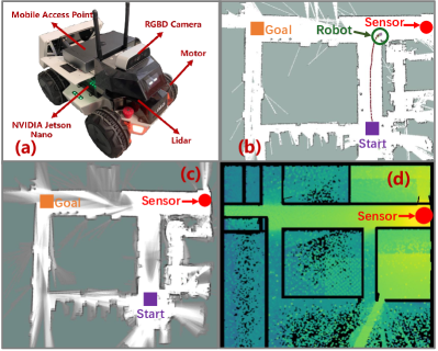
Figure 1: MPCOM leverages grid and radio maps to realize communication- and shape-aware trajectory generation.

To satisfy the new requirements of RDG, it is necessary to integrate communication and navigation features for joint optimization. This ignites extensive studies on communication-aware motion planning (CAMP) [3, 10, 11, 12, 13, 14, 15, 16]. However, to maximize the RDG efficiency (i.e., the amount of harvested data per second) using CAMP, we need a mathematical model of radio propagation. Existing works simplify the robot-sensor communication model to a fixed communication coverage [1, 14, 17], or based solely on distance [5, 6, 10, 13]. These models break down if non-line-of-sight (NLOS) signal propagation [4] (shadowing, reflection, diffraction) occur, e.g., a wall blocking the signal between the transceiver. There exist learning-based radio propagation models [3, 4, 18] that account for NLOS. However, they have no explicit form, and not compatible to state-of-the-art motion planning frameworks. Another drawback of existing CAMP methods is the loosely-coupled communication-locomotion, which can be seen from two perspectives. On one hand, communication-centric CAMP approaches, e.g., [1, 2, 5, 6, 10, 12, 13, 14, 16, 15], focus on static-environment CAMP, which ignore dynamic-obstacle collision avoidance. On the other hand, robotic-centric CAMP approaches, e.g., [3, 11, 17], consider collision avoidance, but they fail in directly maximizing the throughput, e.g., they just use signal strength for monitoring connectivity. Finally, from an engineering perspective, most existing works [1, 2, 5, 6, 10, 12, 13, 14, 16, 16, 15] focus on computation of a predetermined communication-aware trajectory. For real-time robot control in a dynamic environment, they break down due to insufficient execution frequency (e.g., $1\,$Hz or so).

To fill the gap, this paper proposes radio map guided model predictive communication (RM-MPCOM, or MPCOM for short), which is a tightly-coupled communication-locomotion solution (Fig. 1a shows our robot collector and Fig. 1b shows its communication-aware trajectory) that leverages both grid (Fig. 1c) and radio (Fig. 1d) maps for simultaneous shape-aware collision avoidance and radio-aware throughput maximization. Essentially, the proposed MPCOM trades off the following three objectives: 1) reaching goal; 2) avoiding collision; 3) improving radio environment. Contributions of this paper are summarized below.

• MPCOM leverages ray tracing for radio mapping, and proposes an approximate map-partition communication model to learn from the radio map for capturing NLOS propagation characteristics.

• To integrate the radio map into the MPCOM framework, we propose a logarithms-of-polynomials communication regularizer. To address its nonconvexity, a majorization minimization (MM) tehcnique is proposed, which optimizes surrogate regularizers iteratively. The iteration is guaranteed to converge and is able to find the right balance between spending time on motion versus on communication.

• We verify MPCOM in IRSIM and CARLA simulators. Results show that the proposed MPCOM outperforms extensive benchmark schemes in both LOS and NLOS cases, which demonstrates the necessity of leveraging radio maps for CAMP. We also implement MPCOM in ROS and illustrate its robustness in real-world settings.

II Related Work

Motion planning aims to generate collision-free trajectories from the current position to the goal position [7, 8, 9]. The problem consists of state evolution, dynamics limits, and collision avoidance constraints, of which the bottleneck lies at the collision avoidance part. In particular, if the collision avoidance adopts the point-based obstacle model, then the resultant point-mass MP is prone to get stuck especially when the number of non-ball-shape obstacles is large [7]. On the other hand, if the collision avoidance adopts the non-point-based obstacle model that takes the shapes of objects into account, the resultant shape-aware MP problem is nontrivial to solve, as it relies on nonconvex numerical solvers [7]. To reduce the computational complexity, parallel optimization algorithms, such as the alternating direction method of multipliers (ADMM) [8], penalty dual decomposition (PDD) [17], and model-based learning [19], have been employed to decompose the shape-aware problem into parallel problems. Unfortunately, all the above methods plan robot trajectories merely according to the navigation requirements, thus failing in maximizing the communication efficiency in RDG systems.

CAMP emerges to overcome the drawbacks of MP in RDG [1, 2, 5, 3, 6, 10, 11, 12, 13, 14, 15, 16, 17]. These approaches aim to simultaneously minimize the communication and distance costs, under both robot dynamics and channel fading constraints, which signifies a intertwined design considering both the MP of the ego-robot and the DG between the ego-robot and sensors. Current CAMP can be categorized into communication-centric [2, 6, 10, 13, 15, 16] and robotic-centric approaches [5, 1, 3, 11, 12, 14, 16, 17, 15]. The former methods adopt accurate throughput model for optimization. For instance, trajectory planning problems of ground [2, 6, 16] and aerial [10, 13] robots are studied to concurrently optimize the communication efficiency and energy consumption of the RDG systems. Nevertheless, these works are tailored for a static environment, which ignore collision avoidance. On the other hand, robotic-centric methods [1, 3, 11, 12, 14, 16, 17, 15] consider collision avoidance in environments with dynamic obstacles while taking communication factors into account. For instance, an adaptive navigation framework was proposed in [11] and a communication-aware multi-robot exploration framework was presented in [3]. However, these methods treat communication as an auxiliary sub-task, which is not communication-efficient and degrades the RDG efficiency. Their collision avoidance modules also ignore the shape of object, e.g., [5, 1, 14].

Our MPCOM belongs to the CAMP approaches. However, in contrast to existing CAMP with loosely-coupled communication-locomotion, MPCOM is tightly-coupled due to the following: 1) It leverages both grid and radio maps for dual map guided MPCOM; 2) It integrates obstacle shape and communication throughput into the unified communication-locomotion joint optimization framework; 3) It realizes real-time (above $20\,$Hz) automatic balance between communication and navigation based on an iterative MM procedure with theoretical guarantee.

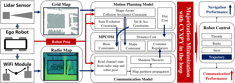
Figure 2: System architecture of MPCOM, which is a tightly-coupled planning-communication system.

III System Overview

The architecture of MPCOM is shown in Fig. 2, which is a strongly-coupled communication-planning system. The system inputs (on the left hand side of Fig. 2) consist of:

• Grid map. The grid map defines the occupancy and feasible areas of the environment. It is built by simultaneous localization and mapping (SLAM), which is a technology based on onboard lidar sensor and spatial computing algorithms, e.g., gmapping (Fig. 2), cartographer (Fig. 1c), or fast-lio [20].

• Robot pose. The robot pose (including position and orientation) is obtained from the extended Kalman filter using onboard inertial sensor and scan matching between lidar measurements and the grid map.

• Radio map. The radio map defines the function to map the robot-sensor locations to the corresponding signal attenuation. It is built by ray-tracing approaches, which is a technology based on 3D reconstruction and wave propagation simulation.

The system outputs consist of collision-free trajectories and associated actions including steer, throttle, and brake (on the right hand side of Fig. 2). The goal of MPCOM is to optimize the conflicting objectives of navigation time minimization, collision-ratio minimization, and communication throughput maximization. The automatic trade-off between these objectives is realized by integrating the cost functions and physical constraints of both motion planning and data communication models into a unified MPC framework through the design of an aggregated objective function. As shown in the middle of Fig. 2, this function consists of a path-tracking distance cost for navigation, a shape-aware constraint for collision avoidance, and a communication regularizer for data collection. The problem is then solved using the MM framework, leading to an iterative refinement procedure, with each iteration solving convexified surrogate problems.

IV Robot Motion and Communication Models

We consider a robotic wireless data gathering system, which consists of $1$ robot collector and $K$ sensor devices, operating in an environment with $M$ dynamic obstacles. At the $t$-th time slot, the robot state is denoted as $\mathbf{s}_{t}=(x_{t},y_{t},\theta_{t})$. where $(x_{t},y_{t})$ and $\theta_{t}$ are positions and orientations of the robot. The robot action at the $t$-th time slot is $\mathbf{u}_{t}=(v_{t},\psi_{t})$. where $v_{t}$ and $\psi_{t}$ are the linear and angular velocities, respectively. The position of the $k$-th sensor device is given by $\mathbf{z}_{k}=(a_{k},b_{k})$ . The navigation environment is described by a map with a set of obstacles $\mathcal{O}=\{\mathbf{o}_{1},...,\mathbf{o}_{M}\}$ and waypoints $\mathcal{W}=\{\mathbf{w}_{1},\mathbf{w}_{2},\cdots\}$, where $\mathcal{O}$ and $\mathcal{W}$ are generated by the object detection and global planning modules, respectively. The state of the $m$-th obstacle, $\mathbf{o}_{m}$, has the same structure as $\mathbf{s}_{t}$. The $i$-th waypoint is $\mathbf{w}_{i}=(x_{i}^{*},y_{i}^{*},\theta_{i}^{*})$, where $(x_{i}^{*},y_{i}^{*})$ and $\theta_{i}^{*}$ are the associated positions and orientations.

The robot motion is subject to three types of constraints: (1) state evolution constraints due to wheel dynamics; (2) action boundary constraints; (3) collision avoidance constraints. First, the state evolution model $\mathbf{s}_{t+1}=E(\mathbf{s}_{t},\mathbf{u}_{t})$ is adopted to predict the trajectories $\{\mathbf{s}_{t+1},\cdots,\mathbf{s}_{t+H}\}$ given the current state $\mathbf{s}_{t}$, where $E$ is determined by Ackermann kinetics:

$$E\left(\mathbf{s}_{t},\mathbf{u}_{t}\right)=\mathbf{A}_{t}{\mathbf{s}_{t}}+\mathbf{B}_{t}{\mathbf{u}_{t}}+\mathbf{c}_{t},~{}\forall t,$$ (1)

where $(\mathbf{A}_{t}$, $\mathbf{B}_{t}$, $\mathbf{c}_{t})$ are coefficient matrices defined in equations (8)–(10) of [8, Sec. III-B]. With the above state evolution model, we can compute state $\mathbf{s}_{t+h+1}=E(\mathbf{s}_{t+h},\mathbf{u}_{t+h})$ for any $h\in[0,H-1]$, where $H$ is the length of prediction horizon. Second, the robot action vector is bounded by

$$\left\{\begin{array}[]{ll}\mathbf{u}_{\min}\preceq\mathbf{u}_{t+h}\preceq\mathbf{u}_{\max},~{}\forall h\\ \mathbf{a}_{\min}\preceq{\mathbf{u}_{t+h+1}}-{\mathbf{u}_{t+h}}\preceq\mathbf{a}_{\max},~{}\forall h\end{array}\right.,$$ (2)

where ${\mathbf{u}_{\min}}$ and ${\mathbf{u}_{\max}}$ are the minimum and maximum values of the control vector, respectively, and ${\mathbf{a}_{\min}}$ and ${\mathbf{a}_{\max}}$ are the associated minimum and maximum acceleration bounds. Third, denote ${\bf{dist}}\left(\mathbf{s}_{t},\mathbf{o}_{m}\right)$ as the exact distance (i.e., the shapes of objects are taken into account) between the robot and the $m$-th obstacle at the $t$-th time slot. To avoid collision with any obstacle $m$ with $m\in\{1,\cdots,M\}$ at any time $(t+h)$ with $h\in[0,H]$, we have

$${\bf{dist}}\left(\mathbf{s}_{t+h},\mathbf{o}_{m}\right)\geq d_{\mathrm{safe}},~{}\forall m,h,$$ (3)

where $d_{\mathrm{safe}}$ in meter is a pre-defined safety distance.

When the robot moves to the position $(x_{t},y_{t})$ at the $t$-th time slot, it will collect data from all IoT devices for a duration of $\tau$, where $\tau$ is the time step between consecutive robot states. The value of $\tau$ is inversely proportional to the operation frequency of motion planning. Within this $\tau$, RF sources at all IoT devices transmit symbols $\{z_{k,t}\in\mathbb{C}\}$ with $\mathbb{E}[|z_{k,t}|^{2}]=p_{k}$ using frequency division multiple access (a widely used multiplexing scheme for WiFi), where $p_{k}$ is the transmit power of the $k$-th IoT device. Then the received signal-to-noise ratio (SNR) at the robot receiver is $\mathsf{SNR}_{k}=G_{t,k}p_{k}/\sigma^{2}$, where $G_{t,k}$ is the uplink channel gain from the $k$-th sensor to the robot collector, and $\sigma^{2}$ is the power of complex Gaussian noise including the inter-user interference. The channel can be estimated as $G_{t,k}=\mathsf{RM}(x_{t},y_{t},a_{k},b_{k})$, where $\mathsf{RM}$ is the radio map function $\mathsf{RM}$ with respect to the robot-sensor locations $[(x_{t},y_{t}),(a_{k},b_{k})]$. Using the Shannon capacity theorem, the spectral efficiency in bps/Hz of the $k$-th device is

$$R_{k,t}=\mathrm{log}_{2}\left(1+\frac{\mathsf{RM}(x_{t},y_{t},a_{k},b_{k})p_{k}}{\sigma^{2}}\right).$$ (4)

V Radio Mapping

V-A Radio Map Multi-Zone Propagation Model

In general, the radio map $\mathsf{RM}$ is a nonlinear function of $(x_{t},y_{t})$ and $(a_{k},b_{k})$ [4, 18, 21]. Particularly, this nonlinear function should satisfy the following properties:

• In the LOS case, $\mathsf{RM}(x_{t},y_{t},a_{k},b_{k})$ is dominated by the direct link and is given by

  $$\mathsf{RM}(x_{t},y_{t},a_{k},b_{k})=\varrho_{0}\,\|x_{t}-a_{k},y_{t}-b_{k}\|_{2}^{-\lambda},$$ (5)

  where $\varrho_{0}$ (the pathloss at a distance of $1\,$meter) and $\lambda\in[2,5]$ (the path loss exponent) are parameters to be fitted by experiment data;

• In the NLOS case, there exists higher-order propagation and blockage effects, and we have:

  $$\mathsf{RM}(x_{t},y_{t},a_{k},b_{k})=f_{\mathsf{nlos}}(x_{t},y_{t},a_{k},b_{k})$$

  $$\quad\times\varrho_{0}\|x_{t}-a_{k},y_{t}-b_{k}\|_{2}^{-\gamma(x_{t},y_{t},a_{k},b_{k})},$$ (6)

  where $\gamma(x_{t},y_{t},a_{k},b_{k})$ is the NLOS exponent (with $\gamma=0$ representing no distance dependence), and the continuous function $f_{\mathsf{nlos}}(x_{t},y_{t},a_{k},b_{k})$ accounts for aggregation of complex radio propagation effects. They do not have an explicit form.

• The radio map $\mathsf{RM}$ is highly dependent on the 3D topology of the environment, and enjoys the partition effect as shown in Fig. 3. This means that the NLOS value $f_{\mathsf{nlos}}$ is identical for two positions within the same zone (e.g., room, corridor). This is because the NLOS signal power attenuation is mainly caused by reflections/diffraction from buildings, and obstacles blocking the direct link between robot and sensor.

Based on the properties (i)–(iii), the following nonlinear model $\Theta(\{\beta_{l},\alpha_{l}\})$ can be used to capture the pattern of $\mathsf{RM}$:

$$\mathsf{RM}(x_{t},y_{t},a_{k},b_{k})\approx\Theta(x_{t},y_{t},a_{k},b_{k}|\{\beta_{l},\alpha_{l}\})$$

$$\quad\quad=\sum_{l=1}^{L}\beta_{l}\mathbb{I}_{\mathcal{Z}_{l}}(x_{t},y_{t})\|x_{t}-a_{k},y_{t}-b_{k}\|_{2}^{-\alpha_{l}},$$ (7)

where the indicator function $\mathbb{I}$ is given by

$$\mathbb{I}_{\mathcal{Z}_{l}}(x_{t},y_{t})=\left\{\begin{array}[]{ll}1,&\mathrm{if}~{}(x_{t},y_{t})\in\mathcal{Z}_{l}\\ 0,&\mathrm{if}~{}(x_{t},y_{t})\notin\mathcal{Z}_{l}\end{array}\right.,$$ (8)

and $\{\mathcal{Z}_{1},\mathcal{Z}_{2},\cdots,\mathcal{Z}_{L}\}$ are submaps with the $l$-th submap ($L$ is the total number of submaps) defined by a set $\mathbb{Z}_{l}=\{\mathbf{z}\in{\mathbb{R}^{2}}|\mathbf{G}_{l}\mathbf{z}\leq{\mathbf{g}_{l}}\}$, where $\mathbf{G}_{l}\in{\mathbb{R}^{E\times 2}}$ and $\mathbf{g}_{l}\in{\mathbb{R}^{E}}$, with $E$ being the number of edges for the submap. The values of $\{\mathbf{G}_{l},\mathbf{g}_{l}\}$ are obtained by applying the image segmentation to the radio map. Note that $\mathcal{Z}_{1}$ represents the LOS region with $\beta_{1}=\varrho_{0}$ and $\alpha_{1}=\lambda$. It can be seen that $\Theta$ satisfies all the properties.

V-B Parameter Fitting of Radio Maps

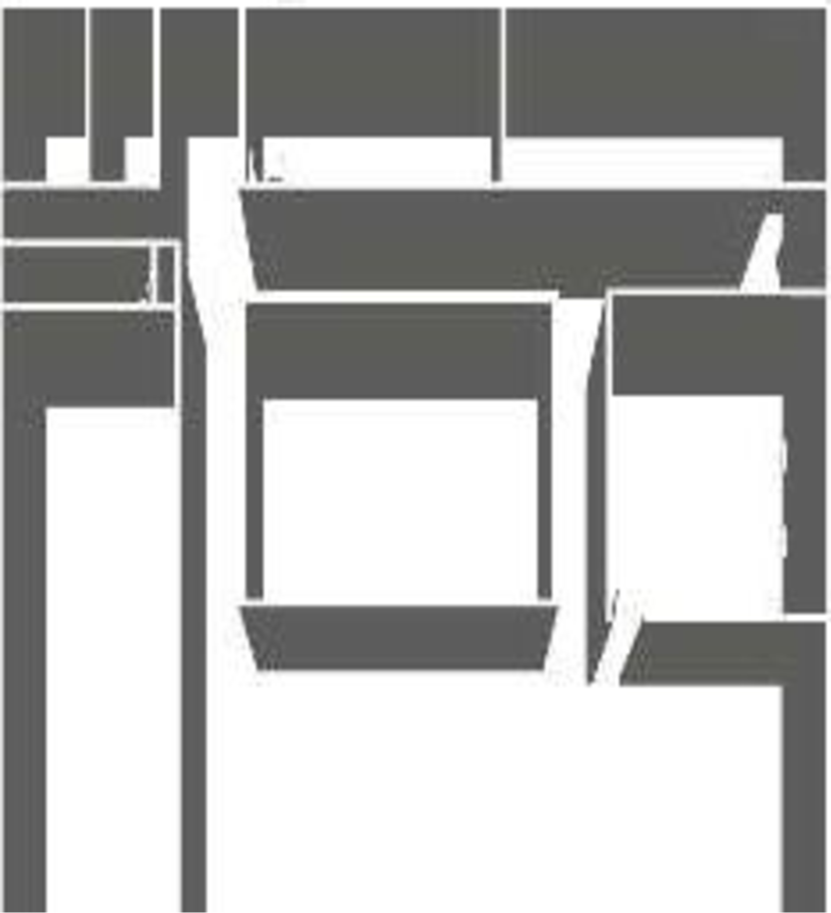
(a) 3D map

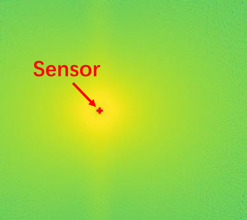
(b) Wide-open

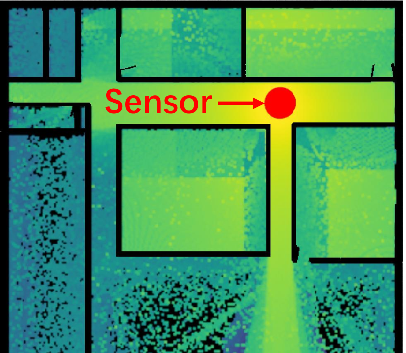
(c) Corridor

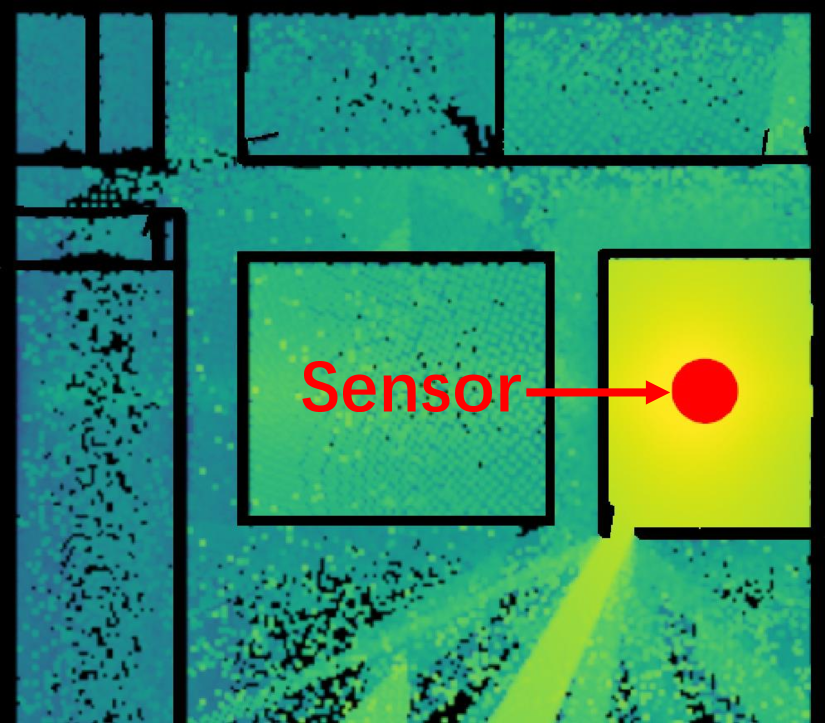
(d) Room

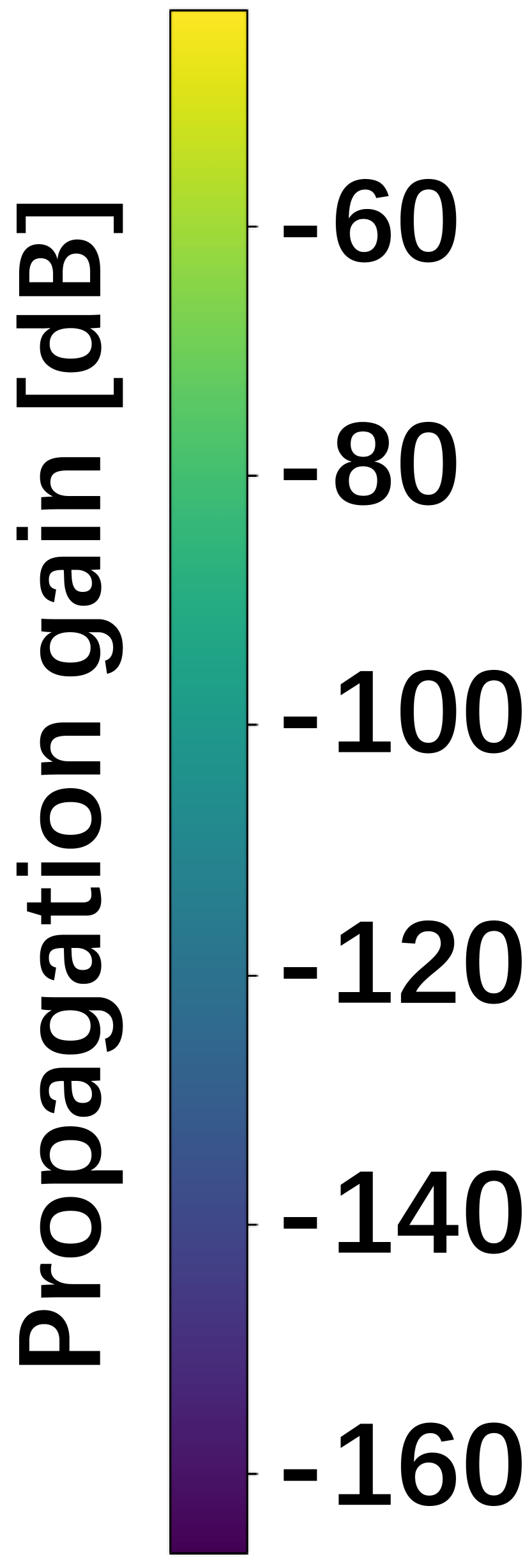
(e)

Figure 3: 3d and radio maps of wide-open, corridor, and room.

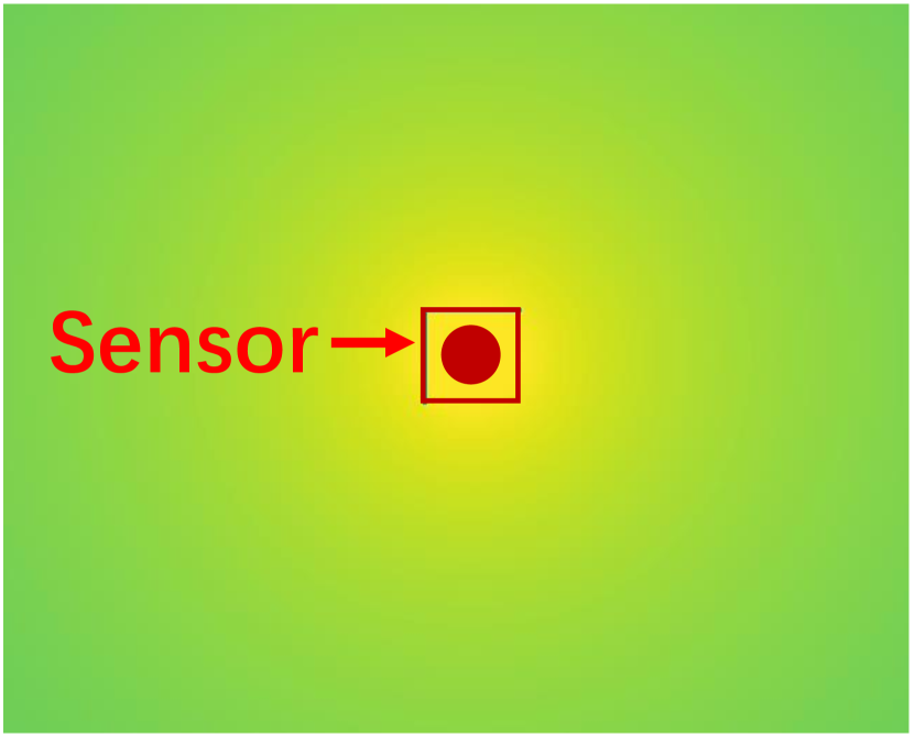
(a) Wide-open

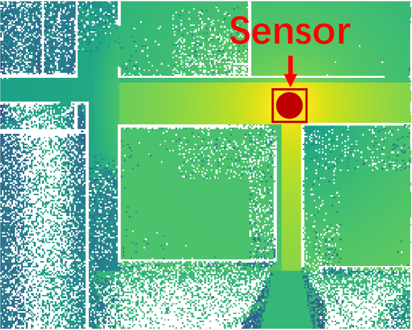
(b) Corridor

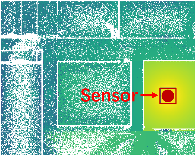
(c) Room

Figure 4: Fitted radio maps of multi-zone propagation model.

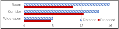
Figure 5: Fitting errors (in dB) of different schemes.

To verify the proposed propagation model in (7), we consider the office environment in Fig. 3a and use the nvidia sionna, a widely used ray tracing package, to obtain the ground truth radio maps. We vary the value of sensor position (i.e., marked as a red ball in Fig. 3) as $\{(a_{k}^{(1)},b_{k}^{(1)}),(a_{k}^{(2)},b_{k}^{(2)}),(a_{k}^{(3)},b_{k}^{(3)})\}=\{(-3,-3),(20.5,-9.0),(26.1,-5)\}$, and obtain the corresponding radio maps $(\mathsf{RM}^{(1)},\mathsf{RM}^{(2)},\mathsf{RM}^{(3)})$ in wide-open, corridor, and room cases, respectively, as shown in Fig. 3b, 3c, 3d (the dB bar is shown in Fig. 3e). With $(\mathsf{RM}^{(1)},\mathsf{RM}^{(2)},\mathsf{RM}^{(3)})$ , the parameters $(\{\beta_{l},\alpha_{l}\})$ in $\Theta$ can be found via the following nonlinear least squares fitting:

$$\mathop{\mathrm{min}}_{\{\beta_{l},\alpha_{l}\}}\quad \frac{1}{Q}\mathop{\sum}_{j=1}^{Q}\Big{|}\mathsf{RM}^{(i)}(x_{j},y_{j})-\Theta^{(i)}(x_{j},y_{j}|\{\beta_{l},\alpha_{l}\})\Big{|}^{2},$$

$$\mathrm{s.t.}\quad \beta_{\min}\leq\beta_{l}\leq\beta_{\max},\forall l,~{}\beta_{1}=\varrho_{0},~{}\alpha_{1}\in[2,5].$$ (9)

Note that under fixed sensor position $(a_{k},b_{k})$, $\mathsf{RM}^{(i)}$ and $\Theta^{(i)}$ are only related to robot position $(x_{j},y_{j})$. The above problem can be solved by 2D brute-force search, or gradient descent method. Since the parameters $(\{\beta_{l},\alpha_{l}\})$ for different maps are obtained independently, the total complexity is linear in terms of the number of radio maps.

We fit the proposed multi-zone model in (7) to the radio maps in Fig. 3. It can be seen that the multi-zone model in (7) matches the experimental data in Fig. 3 very well for all the three scenarios. Moreover, we compare the proposed model with the distance-based model

$$\mathsf{RM}(x_{t},y_{t},a_{k},b_{k})\approx\varrho_{0}\|x_{t}-a_{k},y_{t}-b_{k}\|_{2}^{-\lambda}.$$ (10)

The fitting errors of two models for the three cases are shown in Fig. 5. The multi-zone model achieves the minimum fitting error for all the three cases. The distance-based model achieves a similar fitting error in the wide-open scenario. However, it results in high fitting errors in the corridor and room cases. This implies that the distance-based model does not capture high-order propagation characteristics in NLOS cases.

VI Radio Map Regularization

VI-A Problem Formulation

In the considered system, our task is to maximize the total amount of data harvested from all sensors, while minimizing the distances between the actual robot footprints and the target waypoints, by planning the robot trajectory, involving variables $\{\mathbf{s}_{t+h}\}_{h=0}^{H}$ and $\{\mathbf{u}_{t+h}\}_{h=0}^{H}$. This cannot be realized by conventional MPC that merely minimizes the distance cost

$$C_{0}\left(\{\mathbf{s}_{t+h}\}_{h=0}^{H}\right)=\sum^{H}_{h=0}\left\|\mathbf{s}_{t+h}-\mathbf{s}_{t+h}^{\diamond}\right\|^{2},$$ (11)

where $\{\mathbf{s}_{i}^{\diamond}\}$ represents the list of local waypoints that are extracted from the global waypoints $\mathcal{W}$ according to the current robot state $\mathbf{s}_{t}$. Therefore, this paper proposes to add the following communication awareness regularizer $C_{1}$ to $C_{0}$:

$$C_{1}\left(\{\mathbf{s}_{t+h}\}_{h=0}^{H}\right)=-\rho\sum_{h=0}^{H}\sum_{k=1}^{K}\Phi_{k,t+h}(x_{t+h},y_{t+h})$$ (12)

where $\rho$ is a hyper-parameter to control the trade-off between collecting the sensor data and reaching the goal, and $\Phi_{k,t}$ is short for $\Theta(x_{t},y_{t},a_{k}^{*},b_{k}^{*}|\{\beta_{l}^{*},\alpha_{l}^{*}\})$.

Consequently, the MPCOM problem is formulated as

$$(\mathsf{P}0)\min\limits_{\{\mathbf{s}_{k,t+h},\mathbf{u}_{k,t+h}\}}~{}~{} C_{0}\left(\{\mathbf{s}_{t+h}\}_{h=0}^{H}\right)+C_{1}\left(\{\mathbf{s}_{t+h}\}_{h=0}^{H}\right)$$

s.t. $$\mathsf{constraints}~{}\eqref{dynamics},\eqref{bounds},\eqref{collision}.$$ (13)

Problem $\mathsf{P}0$ is a nonconvex optimization problem, due to the regularizer $C_{1}$ in the cost function and the collision avoidance constraints in (3). Moreover, it is a nonsmooth problem due to the existence of linear constraints in (2), and nonlinear constraints in (1) and (3). Consequently, it is nontrivial to solve $\mathsf{P}0$, and existing methods, e.g., gradient methods, interior point methods, are not applicable. In the following subsection, we will derive a successive optimization approach based on the MM technique, and analyze the associated properties of the derived method.

VI-B Majorization Minimization

To solve $\mathsf{P}0$, we propose to use the framework of MM, which constructs a sequence of upper bounds $\{-\widetilde{\Phi}_{k,t}\}$ on $\{-\Phi_{k,t}\}$ and replaces $\{-\Phi_{k,t}\}$ in $\mathsf{P}0$ with $\{-\widetilde{\Phi}_{k,t}\}$ to obtain a sequence of surrogate problems. In other words, we need to construct lower bounds $\{\widetilde{\Phi}_{k,t}\}$ on $\{\Phi_{k,t}\}$. More specifically, given any feasible solution $\{\mathbf{s}_{k,t+h}^{\star},\mathbf{u}_{k,t+h}^{\star}\}$, to $\mathsf{P}0$, we define surrogate function

$$\widetilde{\Phi}_{k,t}(\mathbf{s}_{t}|\mathbf{s}_{t}^{\star})=\tau B\mathrm{log}_{2}\Bigg{(}1+\frac{\sum_{l=1}^{L}\beta_{l}\mathbb{I}_{\mathcal{Z}_{l}}(x_{t},y_{t})p_{k}}{\sigma^{2}}\times$$

$$\Big{[}2\|\mathbf{s}_{t}^{\star}-\mathbf{c}_{k,t}\|_{2}^{-\alpha_{l}}-\|\mathbf{s}_{t}^{\star}-\mathbf{c}_{k,t}\|_{2}^{-2\alpha_{l}}\left\|x_{t}-a_{k},y_{t}-b_{k}\right\|_{2}^{\alpha_{l}}\Big{]}\Bigg{)},$$ (14)

where $\mathbf{c}_{k,t}=[x_{k},y_{k},\theta_{t}^{\star}]^{T}$, and the following proposition can be established.

Proposition 1.

$\{\widetilde{\Phi}_{k,t}\}$ satisfy the following conditions:

(i) Lower bound condition: $\widetilde{\Phi}_{k,t}(\mathbf{s}_{t}|\mathbf{s}_{t}^{\star})\leq\Phi_{k,t}(\mathbf{s}_{t})$.

(ii) Concavity: $\widetilde{\Phi}_{k,t}(\mathbf{s}_{t}|\mathbf{s}_{t}^{\star})$ is concave in $\mathbf{s}_{t}$.

(iii) Local tightness condition: $\widetilde{\Phi}_{k,t}(\mathbf{s}_{t}^{\star}|\mathbf{s}_{t}^{\star})=\Phi_{k,t}(\mathbf{s}_{t}^{\star})$ and $\nabla\widetilde{\Phi}_{k,t}(\mathbf{s}_{t}^{\star}|\mathbf{s}_{t}^{\star})=\nabla\Phi_{k,t}(\mathbf{s}_{t}^{\star})$.

Proof.

Part (i) is proved based on $\frac{1}{x}\geq\frac{1}{y}-\frac{1}{y^{2}}(x-y)$ for any $(x,y)$. Part (ii) is proved by checking the semi-definiteness of Hessian of $\widetilde{\Phi}_{k,t}$. Part (iii) is proved by computing the function and gradient values of $\widetilde{\Phi}_{k,t}$ and $\Phi_{k,t}$. ∎

With part (i) of Proposition 1, an upper bound can be directly obtained if we replace the functions $\{-\Phi_{m}\}$ by $\{-\widetilde{\Phi}_{m}\}$ around a feasible point. However, a tighter upper bound can be achieved if we treat the obtained solution as another feasible point and continue to construct the next-round surrogate function. This procedure can be iterated until $\|\Phi_{k,t}-\widetilde{\Phi}_{k,t}\|_{2}$ is sufficiently small.

Now, assuming that the solution at the $n^{\mathrm{th}}$ iteration is given by $\{\mathbf{s}_{k,t+h}^{[n]},\mathbf{u}_{k,t+h}^{[n]}\}$, the following problem is considered at the $(n+1)^{\mathrm{th}}$ iteration:

$$(\mathsf{P}1^{[n+1]})\min\limits_{\{\mathbf{s}_{k,t+h},\mathbf{u}_{k,t+h}\}}~{}~{} C_{0}\left(\{\mathbf{s}_{t+h}\}_{h=0}^{H}\right)$$

$$-\rho\sum_{h=0}^{H}\sum_{k=1}^{K}\widetilde{\Phi}_{k,t+h}(\mathbf{s}_{t+h}|\mathbf{s}_{t+h}^{[n]})$$

s.t. $$\mathsf{constraints}~{}\eqref{dynamics},\eqref{bounds},\eqref{collision}.$$ (15)

Based on part (ii) of Proposition 1, the problem $\mathsf{P}1^{[n+1]}$ is convex except for (3). To this end, we adopt the strong duality [7] and the RDA method [8] to handle constraint (3). Then $\mathsf{P}1^{[n+1]}$ can be solved by off-the-shelf software packages (e.g., CVXPY) for numerically solving convex optimization problems [22]. Denoting its optimal solution as $\{\mathbf{s}_{t+h}^{*},\mathbf{u}_{t+h}^{*}\}$, we can set $\{\mathbf{s}_{t+h}^{[n+1]}=\mathbf{s}_{t+h}^{*},\mathbf{u}_{t+h}^{[n+1]}=\mathbf{u}_{t+h}^{*}\}$, and the process repeats with solving the problem $\mathsf{P}1^{[n+2]}$. According to part (iii) of Proposition 1 and [23, Theorem 1], every limit point of the sequence $(\{\mathbf{s}_{t+h}^{[0]},\mathbf{u}_{t+h}^{[0]}\},\{\mathbf{s}_{t+h}^{[1]},\mathbf{u}_{t+h}^{[1]}\},,\cdots)$ is a KKT solution to $\mathsf{P}0$ as long as the starting point $\{\mathbf{s}_{t+h}^{[0]},\mathbf{u}_{t+h}^{[0]}\}$ is feasible to $\mathsf{P}0$.

For the MM algorithm, finding a good feasible starting point is of large importance [24]. We propose a distance-based initialization, which solves the following problem:

$$\min\limits_{\{\mathbf{s}_{t+h},\mathbf{u}_{t+h}\}}~{}~{} C_{0}\left(\{\mathbf{s}_{t+h}\}_{h=0}^{H}\right)+\eta\left\|x_{t}-a_{k},y_{t}-b_{k}\right\|_{2}^{2}$$

s.t. $$\mathsf{constraints}~{}\eqref{dynamics},\eqref{bounds},\eqref{collision},$$ (16)

where $\eta$ is a hyper-parameter. In terms of computational complexity, $\mathrm{P}1[n+1]$ involves $3H(\mathrm{states})+3H(\mathrm{actions})=6H$ variables. Therefore, the worst-case complexity for solving $\mathrm{P}1[n+1]$ is $\mathcal{O}(6H)^{3.5})$. Consequently, the total complexity for solving $\mathrm{P}1$ is $\mathcal{O}(\mathcal{I}\,(6H)^{3.5})$, where $\mathcal{I}$ is the number of iterations needed for MPCOM to converge.

VII Experiments

In this section, we adopt numerical simulations, high-fidelity simulators, and hardware experiments to verify the performance and efficiency of MPCOM. The sensor transmit power is $2\,$mW and the communication bandwidth of each sensor is $0.1\,$MHz. The interference plus noise power is $-50\,$dBm (corresponding to $-100\,$dBm/Hz). The parameter $\rho$ is set to $\rho\in[0.1,2]$. All simulations are implemented on a Ubuntu workstation with a $3.7$ GHZ AMD Ryzen 9 5900X CPU and an NVIDIA $4090$ GPU. We also implement MPCOM on a car-like robot platform (shown in Fig. 1), with its detailed settings specified in Section VII-C.

We compare MPCOM to the following benchmarks:

• Regularized dual alternating direction of multipliers (RDA) [8], which is a state-of-the-art MPC scheme. It models objects as convex sets and determines the collision distance (3) by computing the exact distance between the boundaries of two sets;

• Point-mass CAMP (PCAMP) [5], which is a communication-aware motion planner that ignores the shape of objects. Each obstacle as well as the ego-robot is modeled as a single point. Channels are estimated using distance-based propagation model (10).

• Shape-aware distance-propagation CAMP (SDCAMP), which integrates [5] and [8] for communication- and shape-aware planning. SDCAMP is also based on distance propagation model and can be viewed as an enhanced version of PCAMP.

VII-A Experiment 1: Validation of MPCOM in IRSIM

First, we verify the proposed MPCOM in the LOS cases using intelligent robot simulator IRSIM, a Python-based 2D simulator for robot navigation. The trajectories of MPCOM in a wide-open environment with $1$ sensor ($K=1$) and 0–8 obstacles ($M\in[0,2,4,8]$) are shown in Fig. 6(a)–(d). The sensor is marked as a red circle and the obstacles are marked as black circles. The reference path (i.e., the black line) is generated from a list of target waypoints. The actual robot path is represented by a red line and the robot is marked as a blue box. It can be seen that the robot successfully avoids all obstacles and reaches the goal in a smooth manner. Furthermore, the robot selects the inner path instead of the shortest path for collision avoidance, which allows the robot to get closer to the sensor, thereby collecting more data without introducing much extra time.

We compare the proposed MPCOM with RDA and PCAMP, whose trajectories are shown in Fig. 7. Specifically, the LOS-1 case in Fig. 7a–c is the same as Fig. 6d, while the LOS-2 case in Fig. 7d–f is a new cluttered environment. It can be seen from Fig. 7a and Fig. 7d that RDA selects the outer path in both cases, involving less braking and improving time-efficiency. However, such a trajectory makes the robot farther from the sensor, resulting in a smaller communication throughput. On the other hand, as shown in Fig. 7b and Fig. 7e, the PCAMP scheme leads to a larger distance between the robot and any obstacle than RDA and MPCOM. This is because PCAMP ignores the shape of ego-robot, and needs to adopt a larger safety-distance for collision avoidance.

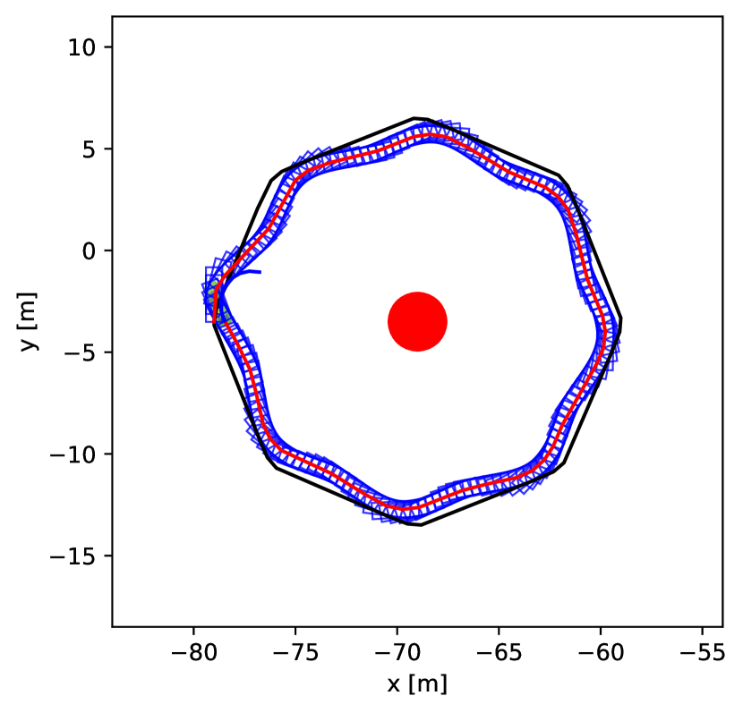
(a) No obstacle

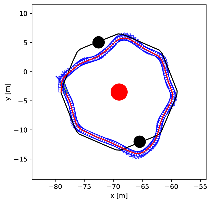
(b) 2 Obstacles

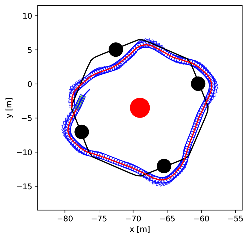
(c) 4 Obstacles

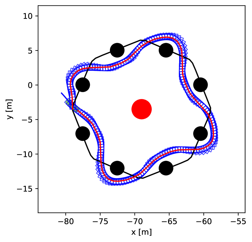
(d) 8 obstacles

Figure 6: Trajectories of MPCOM in LOS cases.

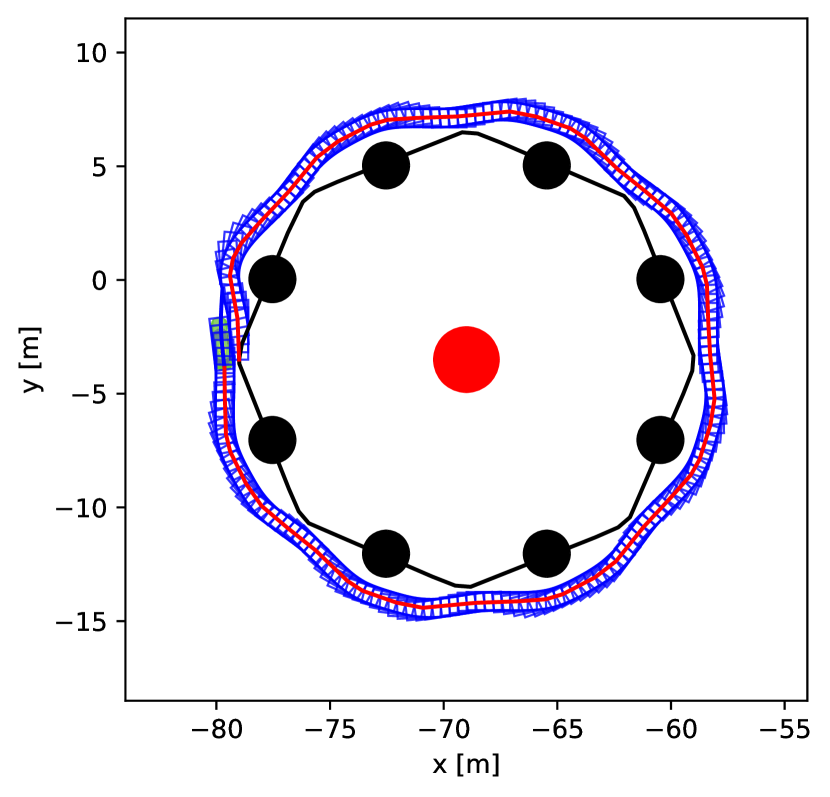
(a) LOS-1 RDA

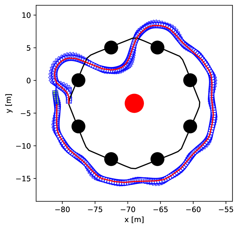
(b) LOS-1 PCAMP

(c) LOS-1 MPCOM

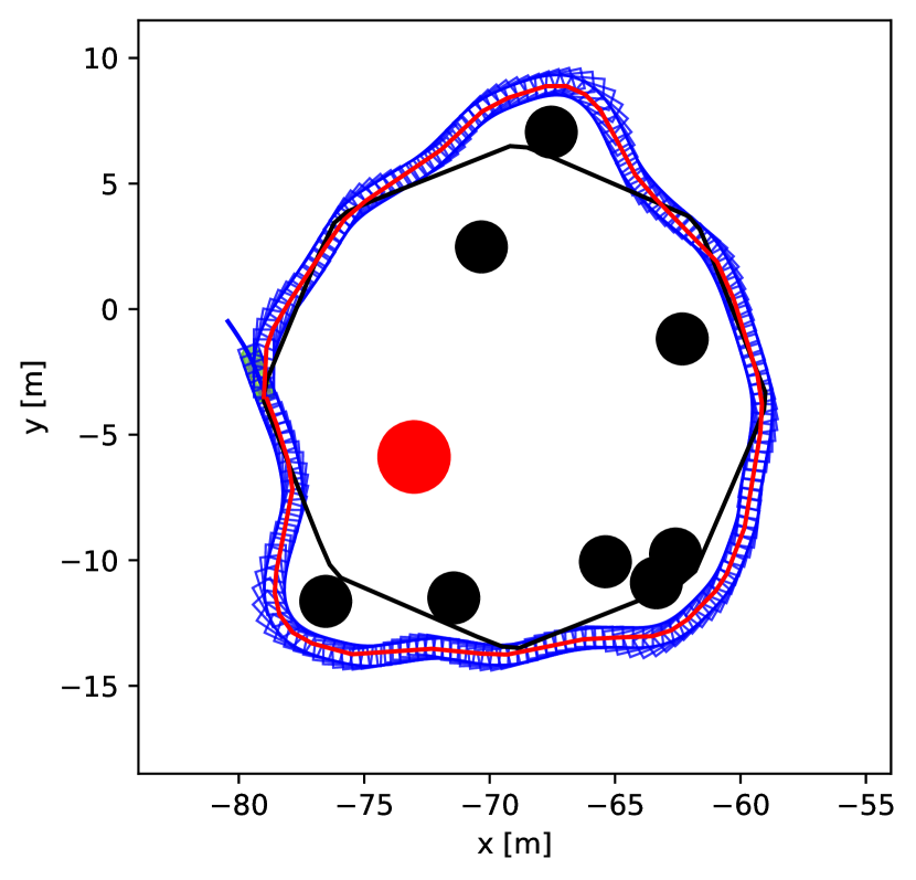
(d) LOS-2 RDA

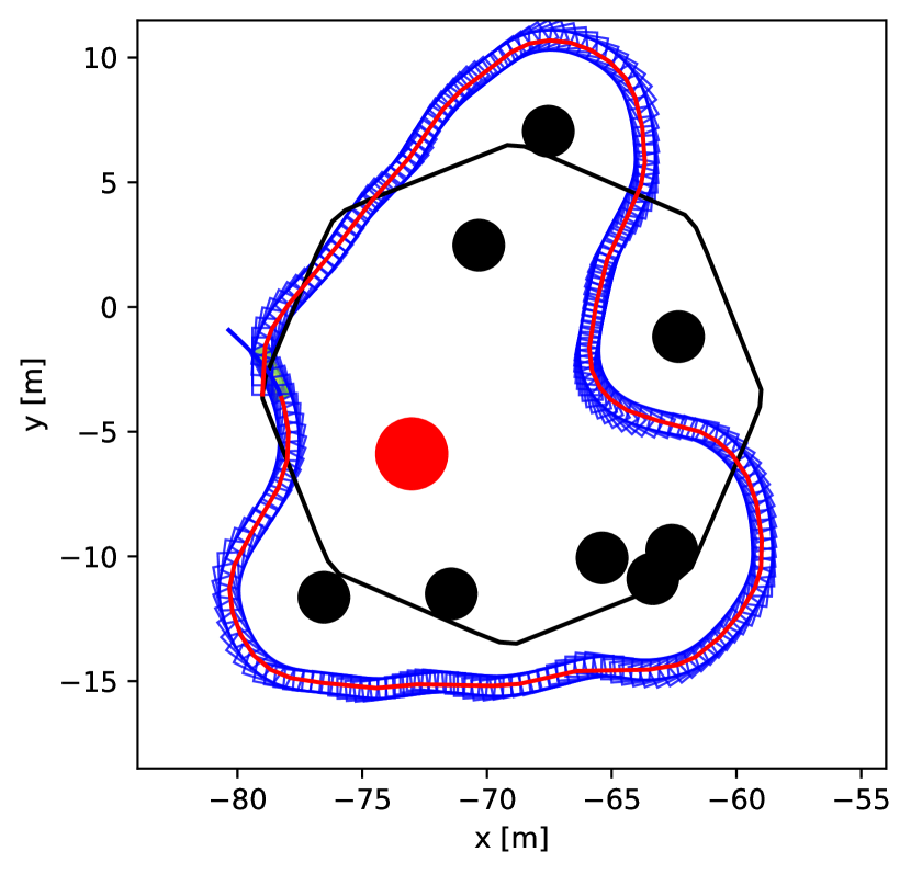
(e) LOS-2 PCAMP

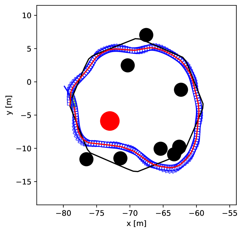
(f) LOS-2 MPCOM

Figure 7: Trajectories of different schemes in two LOS cases.

TABLE I: Quantitative Results in IRSIM.

Sensor†	Obs	RDG Efficiency (MB/s) $\uparrow$				Navigation Time (s) $\downarrow$				Data Throughput (MB) $\uparrow$
		MPCOM (ours)	RDA	PCAMP		MPCOM (ours)	RDA	PCAMP		MPCOM (ours)	RDA	PCAMP
Position A	2	0.378 (+8.31%)	0.349	0.348		15.2	16.0	16.7		5.75	5.59	5.82
Position A	4	0.372 (+8.54%)	0.343	0.334		16.0	16.4	18.3		5.96	5.63	6.12
Position A	8	0.371 (+14.86%)	0.323	0.318		17.5	18.0	22.7		6.50	5.82	7.21
Position B	2	0.284 (+0.35%)	0.273	0.283		15.8	16.0	16.9		4.49	4.37	4.79
Position B	4	0.280 (+3.7%)	0.270	0.268		16.4	16.4	17.7		4.59	4.43	4.75
Position B	8	0.283 (+1.8%)	0.271	0.278		17.7	18.0	22.4		5.01	4.88	6.23
Position C	2	0.278 (+5.3%)	0.264	0.264		16.0	16.0	17.0		4.45	4.22	4.49
Position C	4	0.276 (+3.7%)	0.267	0.258		16.5	16.4	18.6		4.55	4.38	4.79
Position C	8	0.283 (+4.43%)	0.269	0.271		17.7	18.0	21.0		5.01	4.84	5.69
Position D	2	0.286 (+2.51%)	0.269	0.279		15.5	16.0	16.9		4.43	4.31	4.72
Position D	4	0.283 (+5.99%)	0.267	0.262		16.2	16.4	18.4		4.58	4.38	4.82
Position D	8	0.281 (+4.46%)	0.269	0.267		17.9	18.0	22.6		5.04	4.84	6.03

${\dagger}$Sensor positions: A: $(-69,-3.5)$; B: $(-79,6.5)$; C: $(-59,6.5)$; D: $(-59,-13.5)$.

Quantitative results are presented in Table I. It can be seen that no matter how the position of sensor or the number of obstacles changes, the proposed MPCOM always achieves the highest RDG efficiency, with up to $14\%$ efficiency improvement (when the sensor is located at the center) compared with other benchmark schemes. On the other hand, the navigation time of MPCOM is close to RDA, and slightly shorter than RDA in the most cases. This demonstrates that collision avoidance and data collection may not always be contradiction, i.e., they could benefit each other. For instance, in our simulated cases, the sensor is located at the interior of the reference path, and selecting an inner path can simultaneously reduce the navigation time and increase the communication rate. As such, the MPCOM finds the ”Pareto point” between reaching goal and collecting data, resulting in a win-win situlation. In contrast, RDA selects the outer path, which is the optimal collision avoidance path in the short run (as we set the initial position of ego-robot farther than obstacles from the sensor), but in the long run, this is not time- and communication efficient. Lastly, the PCAMP may lead to excessive navigation time due to its lack of consideration for object shapes, which is not desirable in practical RDG applications.

TABLE II: Comparison of different schemes in NOLS-1

	MPCOM	SDCAMP	RDA
RDG Efficiency (MB/s)	0.508 (+101.5%)	0.252	0.239
Avg. Nav. Time (s)	22.6 (+34.5%)	16.8	16.3
Throughput (MB)	11.480 (+171.1%)	4.235	3.895
Task Completion	✔	✗	✗

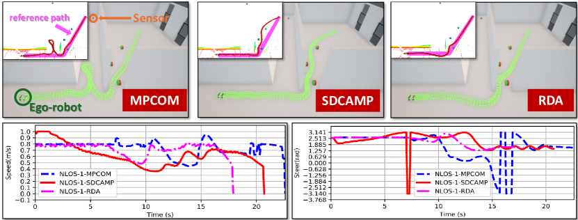
Figure 8: Trajectories and speed profiles of the MPCOM, SDCAMP, and RDA schemes in the NLOS-1 case.

VII-B Experiment 2: Validation of MPCOM in CARLA

Next, we verify the effectiveness of MPCOM in the NLOS cases using CARLA [24, 25], a 3D high-fidelity simulator that adopts Unreal Engine for high-performance rendering and physical engine for accurate dynamics modeling. We consider two NLOS cases. First, we consider the case of $K=1$, where the sensor is located at the corridor. The ground truth and multi-zone radio maps are given by Fig. 3c and Fig. 4b, respectively. The RDG task is deemed as failure if the robot collect less than $10\,$MB data or does not reach the goal within $30\,$s. The trajectories and speed profiles of the three different schemes are shown in Fig. 8. The quantitative results are shwon in Table II. It can be seen that the ego-robot with RDA directly rushes to the goal point at a speed about $0.8\,$m/s, finishing the task in only $16.3\,$s. However, it only collects $3.895\,$MB data, which does not meet the task requirement. The SDCAMP scheme steers and approaches the sensor at the beginning due to its “communication-aware” property. Unfortunately, its distance-based channel estimation is inaccurate, which fails in predicting the impact of NLOS propagation. Consequently, despite the fact that ego-robot is close to the sensor, limited data has been added ($+0.34\,$MB) due to the wall blockage between the sensor and the robot. Meanwhile, it requires extra time to reach the goal. Finally, the proposed MPCOM steers at the T junction and approaches the sensor at corridor due to its joint communication-aware and radio-map-aware property. As a result, the proposed MPCOM successfully accomplish the RDG task, achieving an RDG efficiency significantly higher (+$100\,\%$) than the other benchmark schemes.

To verify the effectiveness of MPCOM in multi-sensor case, we consider the case of $K=4$, where the sensors are randomly distributed at the corridor. The trajectories and speed profiles of the three different schemes are shown in Fig. 9a. The RDG efficiency, navigation time, and total throughput of MPCOM are $11.74\,$MB/s, $24\,$s, and $281.81\,$MB, respectively. Those of RDA are $10.37\,$MB/s, $18.80\,$s, and $195.00\,$MB, respectively. Again, the performance improvement brought by MPCOM is significant, with over $10\,\%$ efficiency gain.

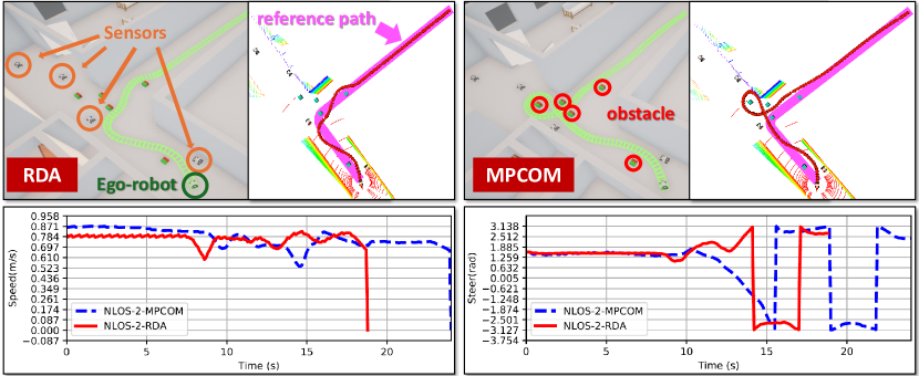
(a) Trajectories and speed profiles of the MPCOM and RDA schemes in the NLOS-2 case.

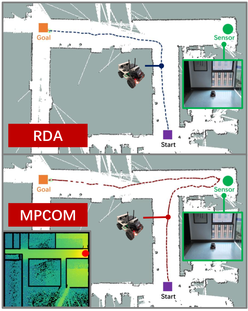
(b) Real-world experiments.

Figure 9: CARLA and Real-world experiments in indoor office environments.

VII-C Experiment 3: Real-World Experiment

Finally, we implement MPCOM on a car-like robot platform (shown in Fig. 1a). The four-wheel robot LIMO has a 2D lidar, RGBD camera, an onboard NVIDIA Jetson-Nano computing platform, and a mobile access point to provide a local wireless network. In this RDG task, the robot needs to collect $30$ images from the sensor (marked as a green ball in Fig. 9), which is represented by a LIMO robot uploading its image topics at a fixed ROS frequency $2\,$Hz. The system is implemented by Python/C$++$ in ROS and inter-robot data sharing is realized via socket communications. It can be seen from Fig. 9b that the trajectory (marked in red) obtained from MPCOM matches the radio map in Fig. 1d very well. This makes it possible for MPCOM to collect more than $30$ images from the sensor (which is also a LIMO robot uploading its image topics at a fixed ROS frequency in our setting). The robot uses $74\,$s to finish the task. In contrast, the RDA scheme in Fig. 9b ignores the radio map and selects the shortest path from starting to goal points (marked in blue). The robot collects fewer than $5$ images and fails the RDG task. The robot uses $37\,$s to reach the goal.

VIII Conclusion

This paper presented a tightly-coupled communication-locomotion solution MPCOM for RDG. A multi-zone propagation model was proposed, which was shown to fit the radio map very well. Experiments showed that MPCOM achieves real-time high-quality data gathering without any safety issue and works well in both LOS and NLOS cases, which corroborates its simultaneous shape-aware and radio-aware nature. Various indoor experiments showed that MPCOM understands the NLOS signal propagation characteristics and outperforms other state-of-the-art CAMP approaches. By integration with reinforcement learning and extension to other tasks, the developed MPCOM opens up opportunities for task-oriented robot navigation.

References

- [1] O. Tekdas, W. Yang, and V. Isler, “Robotic routers: Algorithms and implementation,” The International Journal of Robotics Research, vol. 29, no. 1, pp. 110–126, 2010.
- [2] Y. Yan and Y. Mostofi, “Robotic router formation in realistic communication environments,” IEEE Transactions on Robotics, vol. 28, no. 4, pp. 810–827, 2012.
- [3] M. Saboia, L. Clark, V. Thangavelu, J. A. Edlund, K. Otsu, G. J. Correa, V. S. Varadharajan, A. Santamaria-Navarro, T. Touma, A. Bouman, et al., “Achord: Communication-aware multi-robot coordination with intermittent connectivity,” IEEE Robotics and Automation Letters, vol. 7, no. 4, pp. 10184–10191, 2022.
- [4] L. Clark, J. A. Edlund, M. S. Net, T. S. Vaquero, and A.-a. Agha-Mohammadi, “Propem-l: Radio propagation environment modeling and learning for communication-aware multi-robot exploration,” in Robotics: Science and Systems (RSS), 2022.
- [5] D. B. Licea, M. Bonilla, M. Ghogho, S. Lasaulce, and V. S. Varma, “Communication-aware energy efficient trajectory planning with limited channel knowledge,” IEEE Transactions on Robotics, vol. 36, no. 2, pp. 431–442, 2019.
- [6] S. Wang, M. Xia, and Y.-C. Wu, “Backscatter data collection with unmanned ground vehicle: Mobility management and power allocation,” IEEE Transactions on Wireless Communications, vol. 18, no. 4, pp. 2314–2328, 2019.
- [7] X. Zhang, A. Liniger, and F. Borrelli, “Optimization-based collision avoidance,” IEEE Transactions on Control Systems Technology, vol. 29, no. 3, pp. 972–983, 2020.
- [8] R. Han, S. Wang, S. Wang, Z. Zhang, Q. Zhang, Y. C. Eldar, Q. Hao, and J. Pan, “Rda: An accelerated collision free motion planner for autonomous navigation in cluttered environments,” IEEE Robotics and Automation Letters, vol. 8, no. 3, pp. 1715–1722, 2023.
- [9] X. Zhou, Z. Wang, H. Ye, C. Xu, and F. Gao, “Ego-planner: An esdf-free gradient-based local planner for quadrotors,” IEEE Robotics and Automation Letters, vol. 6, no. 2, pp. 478–485, 2020.
- [10] Y. Guo, C. You, C. Yin, and R. Zhang, “Uav trajectory and communication co-design: Flexible path discretization and path compression,” IEEE Journal on Selected Areas in Communications, vol. 39, no. 11, pp. 3506–3523, 2021.
- [11] L. Zeng, H. Chen, D. Feng, X. Zhang, and X. Chen, “A3d: Adaptive, accurate, and autonomous navigation for edge-assisted drones,” IEEE/ACM Transactions on Networking, 2023.
- [12] A. Lendinez, L. Zanzi, S. Moreno, G. Garí, X. Li, R. Qiu, and X. Costa-Pérez, “Enhancing 5g-enabled robots autonomy by radio-aware semantic maps,” in IEEE/RSJ International Conference on Intelligent Robots and Systems (IROS), pp. 6267–6272, 2023.
- [13] D. B. Licea, G. Silano, M. Ghogho, and M. Saska, “Omnidirectional multi-rotor aerial vehicle pose optimization: A novel approach to physical layer security,” in IEEE International Conference on Acoustics, Speech and Signal Processing (ICASSP), 2024.
- [14] D. Datsko, F. Nekovar, R. Penicka, and M. Saska, “Energy-aware multi-uav coverage mission planning with optimal speed of flight,” IEEE Robotics and Automation Letters, 2024.
- [15] J. Yan, L. Zhang, X. Yang, C. Chen, and X. Guan, “Communication-aware motion planning of auv in obstacle-dense environment: A binocular vision-based deep learning method,” IEEE Transactions on Intelligent Transportation Systems, 2023.
- [16] U. Ali, H. Cai, Y. Mostofi, and Y. Wardi, “Motion-communication co-optimization with cooperative load transfer in mobile robotics: An optimal control perspective,” IEEE Transactions on Control of Network Systems, vol. 6, no. 2, pp. 621–632, 2018.
- [17] G. Li, R. Han, S. Wang, F. Gao, Y. C. Eldar, and C. Xu, “Edge accelerated robot navigation with hierarchical motion planning,” arXiv preprint arXiv:2311.08983, 2023.
- [18] R. Levie, Ç. Yapar, G. Kutyniok, and G. Caire, “Radiounet: Fast radio map estimation with convolutional neural networks,” IEEE Transactions on Wireless Communications, vol. 20, no. 6, pp. 4001–4015, 2021.
- [19] R. Han, S. Wang, S. Wang, Z. Zhang, J. Chen, S. Lin, C. Li, C. Xu, Y. C. Eldar, Q. Hao, et al., “NeuPAN: Direct point robot navigation with end-to-end model-based learning,” arXiv preprint arXiv:2403.06828, 2024.
- [20] W. Xu and F. Zhang, “Fast-lio: A fast, robust lidar-inertial odometry package by tightly-coupled iterated kalman filter,” IEEE Robotics and Automation Letters, vol. 6, no. 2, pp. 3317–3324, 2021.
- [21] C. R. Karanam and Y. Mostofi, “A foundation for wireless channel prediction and full ray makeup estimation using an unmanned vehicle,” IEEE Sensors Journal, 2023.
- [22] S. Diamond and S. Boyd, “Cvxpy: A python-embedded modeling language for convex optimization,” The Journal of Machine Learning Research, vol. 17, no. 1, pp. 2909–2913, 2016.
- [23] Y. Sun, P. Babu, and D. P. Palomar, “Majorization-minimization algorithms in signal processing, communications, and machine learning,” IEEE Transactions on Signal Processing, vol. 65, no. 3, pp. 794–816, 2016.
- [24] A. Dosovitskiy, G. Ros, F. Codevilla, A. Lopez, and V. Koltun, “Carla: An open urban driving simulator,” in Conference on Robot Learning (CoRL), pp. 1–16, PMLR, 2017.
- [25] H. Li, R. Han, Z. Zhao, W. Xu, Q. Hao, S. Wang, and C. Xu, “Seamless virtual reality with integrated synchronizer and synthesizer for autonomous driving,” IEEE Robotics and Automation Letters, pp. 1–8, 2024.