On estimation of heavy-tailed stable linear regression

Abstract.

We study the parameter estimation method for linear regression models with possibly skewed stable distributed errors. Our estimation procedure consists of two stages: first, for the regression coefficients, the Cauchy quasi-maximum likelihood estimator (CQMLE) is considered after taking the differences to remove the skewness of noise, and we prove its asymptotic normality and tail-probability estimate; second, as for stable-distribution parameters, we consider the moment estimators based on the symmetrized and centered residuals and prove their $\sqrt{n}$-consistency. To derive the $\sqrt{n}$-consistency, we essentially used the tail-probability estimate of the CQMLE. The proposed estimation procedure has a very low computational load and is much less time-consuming compared with the maximum-likelihood estimator. Further, our estimator can be effectively used as an initial value of the numerical optimization of the log-likelihood.

1. Introduction

1.1. Objective and background

Let $S^{0}_{\alpha}(\beta,\sigma,\mu)$ be the stable distribution with the continuous parameterization, which is given by the characteristic function

(1.1) $$\varphi(u;\theta):=\exp\left\{i\mu u-(\sigma|u|)^{\alpha}\left(1+i\beta{\rm sgn}(u)\tan\dfrac{\alpha\pi}{2}\left(|\sigma u|^{1-\alpha}-1\right)\right)\right\},$$

where $\theta:=(\alpha,\beta,\sigma,\mu)\in(0,2]\times[-1,1]\times(0,\infty)\times\mathbb{R}$. This is called Nolan’s $0$-parametrization [9], which is continuous in all the parameters. Note that the possibly skewed Cauchy case is then defined to be the limiting case for $\alpha\to 1$ through $\lim_{\alpha\to 1}\tan(\alpha\pi/2)(|u|^{1-\alpha}-1)=(2/\pi)\log|u|$:

$$\varphi(u;1,\beta,\sigma,\mu)=\lim_{\alpha\to 1}\varphi(u;\theta)=\exp\left\{i\mu u-\sigma|u|\left(1+i\beta\dfrac{2}{\pi}{\rm sgn}(u)\log(\sigma|u|)\right)\right\}.$$

It is known that $S_{\alpha}(\beta,\sigma,\mu)$ for $\beta\in(-1,1)$ admits an everywhere positive smooth Lebesgue density; we refer to [11] and [12] for details. We denote by $\phi_{\alpha,\beta}(x)$ the probability density function of $S^{0}_{\alpha}(\beta,1,0)$:

(1.2) $$\phi_{\alpha,\beta}(x):=\frac{1}{2\pi}\int e^{-ixu}\varphi(u;\alpha,\beta,1,0)du.$$

We consider the linear regression model

(1.3) $$Y_{j}=X_{j}\cdot\mu+\sigma\epsilon_{j},$$

where $X_{j}\in\mathbb{R}^{q}$ is a non-random sequence, and

(1.4) $$\epsilon_{1},\epsilon_{2},\dots\sim\text{i.i.d.}~{}S_{\alpha}(\beta,1,0).$$

Here and in what follows the dot denotes the usual inner product. We are concerned with estimation of the unknown parameter $\theta:=(\alpha,\beta,\sigma,\mu)\in\Theta$ from a sample $\{(X_{j},Y_{j})\}_{j=1}^{n}$. Throughout, the parameter space $\Theta$ is assumed to be a bounded convex domain whose closure satisfies

$$\overline{\Theta}\subset(0,2)\times(-1,1)\times(0,\infty)\times\mathbb{R}^{q},$$

and also it is assumed that there exists a true value $\theta_{0}=(\alpha_{0},\beta_{0},\sigma_{0},\mu_{0})\in\Theta$. We denote by $P_{\theta}$ the distribution of $\{(Y_{j},\epsilon_{j})\}_{j=1}^{\infty}$ and by $E_{\theta}$ the corresponding expectation operator.

Parameter estimation of the stable regression model (1.3) has a long history. Typically, one employs the maximum-likelihood estimator (MLE) with numerical integration (for the density) and optimization, see [10, Chapter 5] and the references therein and also [8] especially for the symmetric case; see also [7] for the i.i.d.-$S_{\alpha}(\beta,\sigma,\mu)$ setting and [2] for the time series model. However, it can be rather time-consuming and, more seriously, suffers from the local solution problem, the latter being often inevitable for non-concave log-likelihood cases. In this paper, we address this problem by introducing simple and easy-to-compute estimators based on the Cauchy density and the method of lower-order fractional moments (see also Remark 2.6). As a result, we derived the estimator that is $\sqrt{n}$-consistent and that can be used as the initial value for numerical optimization of the log-likelihood function; although we will not prove the asymptotic normality of the proposed estimator, it would be trivial from the proof while the resulting asymptotic covariance matrix takes a rather complicated form.

We will refer to the estimators introduced and studied in Sections 2 and 3 as initial estimators. The initial estimator consists of the Cauchy quasi-maximum likelihood estimator (CQMLE) $\hat{\mu}_{n}$ and $(\hat{\alpha}_{n},\hat{\beta}_{n},\hat{\sigma}_{n})$ obtained from the method of moment, introduced in Sections 2 and 3, respectively. In Table 1, we computed the initial estimator and the MLE when $q=3$ with the explanatory variables $X_{j}$ being generated independently from the uniform distribution $U(1,5)$. The MLE is computed by changing the initial value of the optimization, as indicated in the caption of Table 1. We see the numerical optimization of the MLE may be rather unstable with long computation time if the starting values are far from the unknown true value, while the MLE numerically guided by the initial estimators is much more stable.

Having obtained the easy-to-compute initial estimator at rate $\sqrt{n}$, it would be natural from a theoretical point of view to consider the Newton-Raphson type one-step estimator (for example, [4]) to construct an asymptotically efficient estimator. However, we found that the numerical computation can be unstable and we do not pursue it in this paper; see also Remark 3.4.

Method	$n$	$\hat{\alpha}_{n}$	$\hat{\beta}_{n}$	$\hat{\sigma}_{n}$	$\hat{\mu}_{n}$	Time(s)
Initial estimator	300	0.58	0.79	1.08	(4.63,1.77,3.08)	$7.1\times 10^{-3}$
MLE (i)	300	0.25	-0.80	248.00	(-4.45,-2.94,-2.61)	5198.90
MLE (ii)	300	0.85	0.45	1.53	(5.02,1.98,3.04)	500.20
True value		0.8	0.5	1.5	(5,2,3)

Table 1. Parameter estimates and computational time (second) for the three cases. For the initial values for numerical optimization of MLE, we used: (i) $(1,0,1,(100,100,100))$ for the bad case where initial values are far from the true values; (ii) $(0.58,0.79,1.08,(4.63,1.77,3.08))$ obtained by the proposed initial estimator: the CQMLE and the moment estimator.

1.2. Outline and summary

In Section 2, we estimate the regression coefficient by the CQMLE without assuming that the errors are stable-distributed. We prove the asymptotic normality and the tail-probability estimate of the normalized CQMLE. In Section 3, we estimate the stable distribution parameter $(\alpha,\beta,\sigma)$ by the method of moments through the residual sequence based on the CQMLE and showed the $\sqrt{n}$-consistency of $(\hat{\alpha}_{n},\hat{\beta}_{n},\hat{\sigma}_{n},\hat{\mu}_{n})$. Importantly, it is essential in our proof that the CQMLE satisfies the polynomial-type tail-probability estimate. As a consequence, we obtain a practical $\sqrt{n}$-consistent estimator, that can be computed in a flash as was seen in Table 1. In Section 4, we extensively conduct numerical experiments, by drawing histograms and boxplots of the initial estimator when we estimated the regression coefficient by the CQMLE and, just for comparison, the other two estimators (the least-squares and the least absolute deviation estimators). Also shown are some histograms of the normalized MLE using the initial estimators as the starting value for optimization, from which it can be seen that we had no local-optimum problem.

2. CQMLE of location parameter

Throughout this section, we temporarily forget the assumption (1.4) on the noise distribution. Taking the difference in the model (1.3):

(2.1) $$\Delta_{j}Y=\Delta_{j}X\cdot\mu+\sigma\Delta_{j}\epsilon,$$

where $\Delta_{j}\zeta:=\zeta_{j}-\zeta_{j-1}$ for $\zeta=X$, $Y$, and $\epsilon$. Then, the CQMLE is defined by any element

$$\hat{\mu}_{n}\in\mathop{\rm argmax}_{\mu\in\Theta_{\mu}}H_{n}(\mu),$$

where

(2.2) $$H_{n}(\mu):=\sum_{j=2}^{n}\log\frac{1}{1+(\Delta_{j}Y-\Delta_{j}X\cdot\mu)^{2}}$$

denotes the Cauchy quasi-likelihood; the parameter space $\Theta_{\mu}$ of $\mu$ is now assumed to be a bounded convex domain. This implies that we will estimate $\mu$ as if the noise part “$\sigma\Delta_{j}\epsilon$” in (2.1) obeys the standard Cauchy distribution. We will prove the asymptotic normality of the CQMLE $\hat{\mu}_{n}$ and estimate the tail-probability of $\hat{\mu}_{n}$.

To proceed, we introduce some assumptions. Let $A^{\otimes 2}:=AA^{\top}$.

Assumption 2.1.

1. There exists a positive number $C_{X}$ such that $\sup_{j}|\Delta_{j}X|<C_{X}.$

2. There exists a positive definite matrix $C_{0}$ and a constant $\beta_{1}\in(0,1/2)$ such that

   (2.3) $$\sup_{n\in\mathbb{N}}n^{\beta_{1}}\left|\frac{1}{n}\sum_{j=2}^{n}(\Delta_{j}X)^{\otimes 2}-C_{0}\right|<\infty.$$

3. There exists a matrix $D_{0}$ such that

   (2.4) $$\lim_{n\rightarrow\infty}\frac{1}{n-2}\sum_{j=2}^{n-1}(\Delta_{j}X)(\Delta_{j+1}X)^{T}=D_{0}.$$

4. There exists a continuous function $Y(\mu)$ such that

   (2.5) $$\sup_{n}\sup_{\mu\in\Theta_{\mu}}\left|n^{1/2-\beta_{2}}\left(Y^{\star}_{n}(\mu)-Y(\mu)\right)\right|<\infty$$

   for some constant $\beta_{2}\in[0,1/2)$, where

   (2.6) $$Y^{\star}_{n}(\mu):=-\frac{1}{n}\sum_{j=2}^{n}E_{\theta_{0}}\left[\log(1+\{\sigma_{0}\Delta_{2}\epsilon-\Delta_{j}X\cdot(\mu-\mu_{0})\}^{2})-\log(1+(\sigma_{0}\Delta_{2}\epsilon)^{2})\right],$$

   and that there exists a constant $\lambda>0$ such that $Y(\mu)\leq-\lambda|\mu-\mu_{0}|^{2}$ for all $\mu\in\mathbb{R}^{q}$.

5. $E_{\theta_{0}}\left[|\log(1+\epsilon_{1}^{2})|^{K}\right]<\infty$ for every $K>0$, and the symmetric distribution of the difference $\epsilon_{2}-\epsilon_{1}$ admits a Lebesgue density $\mathfrak{f}$ for which $\mathfrak{f}(1)>0$,

   (2.7) $$\sup_{x\geq 1}\mathfrak{f}(x)\leq\mathfrak{f}(1)\leq\inf_{0\leq x\leq 1}\mathfrak{f}(x),$$

   and there exist positive constants $\mathfrak{c}_{1},\mathfrak{c}_{2}$ and $\mathfrak{b}$ for which $0<\mathfrak{c}_{1}<\mathfrak{c}_{2}<1$ and

   (2.8) $$\inf_{\mathfrak{c}_{1}\leq x\leq\mathfrak{c}_{2}}\mathfrak{f}(x)\geq(1+\mathfrak{b})\mathfrak{f}(1).$$

Remark 2.2.

1. Note that Assumption 2.1 excludes the constant factor (intercept) in “$X_{j}\cdot\mu$”. This is the price we have to pay to handle possibly arbitrarily heavy-tailed and skewed $\epsilon_{j}$ by the simple and explicit Cauchy quasi-likelihood $H_{n}(\mu)$. See Remark 3.5 for a possible remedy for this inconvenience.

2. Assumption 2.1(2.3) and (2.4) are inevitable to identify the asymptotic covariance matrix of $\hat{\mu}_{n}$ in Theorem 2.4. In practice, one computes the quantities $\frac{1}{n}\sum_{j=2}^{n}(\Delta_{j}X)^{\otimes 2}$ and $\frac{1}{n}\sum_{j=2}^{n}(\Delta_{j}X)(\Delta_{j+1}X)^{T}$, and formally checks that the former is positive definite. Although we are assuming that $X_{1},X_{2},\dots$ are non-random, it could be, for example, a sequence of i.i.d. random vectors $(X_{1},Y_{1}),(X_{2},Y_{2}),\dots$ with $(X_{j})_{j=1}^{\infty}$ being independent of $(\epsilon_{j})_{j=1}^{\infty}$. Then, under the assumption that $E_{\theta_{0}}[|X_{1}|^{K}]<\infty$ for sufficiently large $K>0$, one can apply the central limit theorem for one-dependent sequences [4, Section 11] to conclude Assumption 2.1(2.3) (with $\beta_{1}=1/2$) and (2.4) for $C_{0}=E_{\theta_{0}}[(X_{2}-X_{1})^{\otimes 2}]$ and $D_{0}=E_{\theta_{0}}[(X_{2}-X_{1})(X_{3}-X_{2})^{\top}]$.

3. Assumption 2.1(4) is a strong form of the identifiability (model-separation) condition. When $\{(X_{j},Y_{j})\}_{j=1}^{n}$ is i.i.d. as described in the previous item, then we can take $Y^{\star}_{n}(\mu)\equiv Y(\mu)$ with

   (2.9) $$Y(\mu)=-E_{\theta_{0}}\left[\log(1+\{\sigma_{0}\Delta_{2}\epsilon-\Delta_{2}X\cdot(\mu-\mu_{0})\}^{2})-\log(1+(\sigma_{0}\Delta_{2}\epsilon)^{2})\right].$$

4. Assumption 2.1(5) holds if $\mathfrak{f}$ is continuous and strictly decreasing on $[0,\infty)$ with $\sup_{x}|x|^{1+\delta}\mathfrak{f}(x)<\infty$ for some $\delta>0$. In particular, it holds under (1.4).

Lemma 2.3.

Suppose that (1), (4), and (5) in Assumption 2.1 hold. Then, we have the consistency

(2.10) $$\hat{\mu}_{n}\xrightarrow{p}\mu_{0}.$$

Proof.

Let $Y_{n}(\mu):=n^{-1}(H_{n}(\mu)-H_{n}(\mu_{0}))$; we set $n^{-1}$ just for notational brevity, though it is natural to set $(n-1)^{-1}$ instead. Let $\delta_{j}(\mu):=\Delta_{j}Y-\Delta_{j}X\cdot\mu$; then, $\delta_{j}(\mu_{0})=\sigma_{0}\Delta_{j}\epsilon$. We have

(2.11) $$Y_{n}(\mu) =-\frac{1}{n}\sum_{j=2}^{n}\{\log(1+\{\delta_{j}(\mu_{0})-\Delta_{j}X\cdot(\mu-\mu_{0})\}^{2})-\log(1+\delta_{j}(\mu_{0})^{2})\}$$

(2.12) $$=:-\frac{1}{n}\sum_{j=2}^{n}\xi_{j}(\mu)$$

(2.13) $$=-\frac{1}{n}\sum_{j=2}^{n}\{\xi_{j}(\mu)-E_{\theta_{0}}[\xi_{j}(\mu)]\}-\frac{1}{n}\sum_{j=2}^{n}E_{\theta_{0}}[\xi_{j}(\mu)]$$

(2.14) $$=:-\frac{1}{\sqrt{n}}M_{n}(\mu)+Y^{\star}_{n}(\mu).$$

Hence, under Assumption 2.1(4),

(2.15) $$\sup_{\mu\in\Theta_{\mu}}\left|n^{1/2-\beta_{2}}\left(Y_{n}(\mu)-Y(\mu)\right)\right|\leq C\left(n^{-\beta_{2}}\sup_{\mu\in\Theta_{\mu}}|M_{n}(\mu)|+1\right)\quad\text{a.s.}$$

for a universal constant $C>0$. To conclude the consistency, it suffices to show that

(2.16) $$\sup_{n}E_{\theta_{0}}\left[\sup_{\mu\in\Theta_{\mu}}|M_{n}(\mu)|^{K_{1}}\right]<\infty$$

for sufficiently large $K_{1}>0$, which in particular implies that $\sup_{\mu\in\Theta_{\mu}}|Y_{n}(\mu)-Y(\mu)|\xrightarrow{p}0$; see, for example, [13, Theorem 5.7] for the general result for proving the consistency. The estimate (2.16) is too much to ask for the consistency, but it will be used later in Theorem 2.4.

Since $\Theta_{\mu}$ is a bounded convex domain and since $M_{n}(\mu)$ and its partial derivative $\partial_{\mu}M_{n}(\mu)$ is the sum of random variables with zero expected value, we have the following for $K_{1}>q\vee 2$ by Sobolev’s inequality [1, Remark in p.415]:

(2.17) $$E_{\theta_{0}}\left[\sup_{\mu\in\Theta_{\mu}}|M_{n}(\mu)|^{K_{1}}\right] \leq\sup_{\mu\in\Theta_{\mu}}E_{\theta_{0}}[|M_{n}(\mu)|^{K_{1}}]+\sup_{\mu\in\Theta_{\mu}}E_{\theta_{0}}[|\partial_{\mu}M_{n}(\mu)|^{K_{1}}].$$

In what follows, we will write $a_{n}\lesssim b_{n}$ for two possibly random non-negative sequences $(a_{n})$ and $(b_{n})$ if there exists a universal constant $C>0$ for which $a_{n}\leq Cb_{n}$ a.s. We can obtain the following estimate for the first term of (2.17) from Burkholder’s inequality and Jensen’s inequality:

(2.18) $$\sup_{\mu\in\Theta_{\mu}}E_{\theta_{0}}\left[|M_{n}(\mu)|^{K_{1}}\right] =\sup_{\mu\in\Theta_{\mu}}E_{\theta_{0}}\left[\left|\frac{1}{\sqrt{n}}\sum_{j=2}^{n}\{\xi_{j}(\mu)-E_{\theta_{0}}[\xi_{j}(\mu)]\}\right|^{K_{1}}\right]$$

(2.19) $$\lesssim\sup_{\mu\in\Theta_{\mu}}E_{\theta_{0}}\left[\left(\frac{1}{n}\sum_{j=2}^{n}(\xi_{j}(\mu)-E_{\theta_{0}}[\xi_{j}(\mu)])^{2}\right)^{K_{1}/2}\right]$$

(2.20) $$\lesssim\sup_{\mu\in\Theta_{\mu}}\frac{1}{n}\sum_{j=2}^{n}E_{\theta_{0}}[|\xi_{j}(\mu)|^{K_{1}}]$$

(2.21) $$\lesssim\sup_{\mu\in\Theta_{\mu}}\frac{1}{n}\sum_{j=2}^{n}E_{\theta_{0}}[|\log(1+\delta_{j}(\mu)^{2})|^{K_{1}}]$$

(2.22) $$\lesssim\sup_{\mu\in\Theta_{\mu}}\frac{1}{n}\sum_{j=2}^{n}E_{\theta_{0}}[|\log(1+(\delta_{2}(\mu_{0})+\Delta_{j}X\cdot(\mu_{0}-\mu))^{2})|^{K_{1}}]$$

(2.23) $$\lesssim 1+E_{\theta_{0}}[|\log(1+(|\epsilon_{1}|+|\epsilon_{2}|+1)^{2})|^{K_{1}}]$$

(2.24) $$\lesssim 1+E_{\theta_{0}}\left[|\log(1+\epsilon_{1}^{2})|^{K_{1}}\right]\lesssim 1.$$

Similarly, we can obtain

(2.25) $$\sup_{\mu\in\Theta_{\mu}}E_{\theta_{0}}[|\partial_{\mu}M_{n}(\mu)|^{K_{1}}]\lesssim\sup_{\mu\in\Theta_{\mu}}\frac{1}{n}\sum_{j=2}^{n}E_{\theta_{0}}[|\partial_{\mu}\xi_{j}(\mu)|^{K_{1}}]\lesssim 1.$$

We conclude (2.16), hence the proof is complete. ∎

We will use the abbreviation $\delta_{j}(\mu_{0})=\sigma_{0}\Delta_{j}\epsilon=:S_{j}$.

Theorem 2.4.

Suppose that Assumption 2.1 holds. Then, we have

(2.26) $$\sqrt{n}(\hat{\mu}_{n}-\mu_{0})\xrightarrow{\mathcal{L}}N(0,\Gamma_{0}^{-1}\Sigma_{0}\Gamma_{0}^{-1}),$$

where

$$\Sigma_{0} :=4E_{\theta_{0}}\left[\left(\frac{S_{2}}{1+S_{2}^{2}}\right)^{2}\right]C_{0}+4E_{\theta_{0}}\left[\left(\frac{S_{2}}{1+S_{2}^{2}}\right)\left(\frac{S_{3}}{1+S_{3}^{2}}\right)\right](D_{0}+D_{0}^{T}),$$

$$\Gamma_{0} :=2E_{\theta_{0}}\left[\frac{1-S_{2}^{2}}{(1+S_{2}^{2})^{2}}\right]C_{0}.$$

Furthermore, for any $L>0$ the following tail-probability estimate holds

(2.27) $$\sup_{r>0}\sup_{n\in\mathbb{N}}P_{\theta_{0}}\left[|\sqrt{n}(\hat{\mu}_{n}-\mu_{0})|>r\right]\,r^{L}<\infty.$$

Proof.

First, we prove (2.26). From the mean value theorem,

(2.28) $$\partial_{\mu}H_{n}(\hat{\mu}_{n})=\partial_{\mu}H_{n}(\mu_{0})+\int_{0}^{1}\partial_{\mu}^{2}H_{n}(\mu_{0}+t(\hat{\mu}_{n}-\mu_{0}))dt(\hat{\mu}_{n}-\mu_{0}).$$

By the consistency of $\hat{\mu}_{n}$, we may and do suppose that $\partial_{\mu}H_{n}(\hat{\mu}_{n})=0$, so that

(2.29) $$\sqrt{n}(\hat{\mu}_{n}-\mu_{0})=\left(-\frac{1}{n}\int_{0}^{1}\partial_{\mu}^{2}H_{n}(\mu_{0}+t(\hat{\mu}_{n}-\mu_{0}))dt\right)^{-1}\frac{1}{\sqrt{n}}\partial_{\mu}H_{n}(\mu_{0}).$$

We can conclude (2.26) by showing

(2.30) $$\frac{1}{\sqrt{n}}\partial_{\mu}H_{n}(\mu_{0})\xrightarrow{\mathcal{L}}N(0,\Sigma_{0}),$$

(2.31) $$-\int_{0}^{1}\frac{1}{n}\partial_{\mu}^{2}H_{n}(\mu_{0}+t(\hat{\mu}_{n}-\mu_{0}))dt \xrightarrow{p}\Gamma_{0},$$

with $\Gamma_{0}$ being positive definite.

Proof of (2.30). Observe that

(2.32) $$\frac{1}{\sqrt{n}}\partial_{\mu}H_{n}(\mu_{0}) =-\frac{1}{\sqrt{n}}\sum_{j=2}^{n}\partial_{\mu}\log(1+(\Delta_{j}Y-\Delta_{j}X\cdot\mu)^{2})|_{\mu=\mu_{0}}$$

(2.33) $$=\frac{2}{\sqrt{n}}\sum_{j=2}^{n}\frac{S_{j}}{1+S_{j}^{2}}\Delta_{j}X=:\sum_{j=2}^{n}\chi_{n,j}.$$

Since the distribution of $S_{j}=\sigma_{0}\Delta_{j}\epsilon$ is symmetric,

(2.34) $$E_{\theta_{0}}[\chi_{n,j}] =\frac{2}{\sqrt{n}}E_{\theta_{0}}\left[\frac{S_{2}}{1+S_{2}^{2}}\right]\Delta_{j}X=0.$$

We also have

(2.35) $$\lim_{n\rightarrow\infty}E_{\theta_{0}}\left[\left(\sum_{j=2}^{n}\chi_{n,j}\right)^{\otimes 2}\right] =\lim_{n\rightarrow\infty}\frac{4}{n}E_{\theta_{0}}\left[\sum_{i=2}^{n}\sum_{j=2}^{n}\left(\frac{S_{i}}{1+S_{i}^{2}}\right)\left(\frac{S_{j}}{1+S_{j}^{2}}\right)(\Delta_{i}X)(\Delta_{j}X)^{T}\right]$$

(2.36) $$=\lim_{n\rightarrow\infty}\frac{4}{n}\sum_{j=2}^{n}E_{\theta_{0}}\left[\left(\frac{S_{2}}{1+S_{2}^{2}}\right)^{2}\right](\Delta_{j}X)^{\otimes 2}$$

(2.37) $${}\qquad+4E_{\theta_{0}}\left[\left(\frac{S_{2}}{1+S_{2}^{2}}\right)\left(\frac{S_{3}}{1+S_{3}^{2}}\right)\right]$$

(2.38) $${}\qquad\times\bigg{\{}\lim_{n\rightarrow\infty}\frac{1}{n}\sum_{j=2}^{n-1}\{(\Delta_{j}X)(\Delta_{j+1}X)^{T}+(\Delta_{j+1}X)(\Delta_{j}X)^{T}\}\bigg{\}}$$

(2.39) $$=\Sigma_{0}.$$

The Lyapunov condition holds: for any $\delta>0$,

(2.40) $$\sum_{j=2}^{n}E_{\theta_{0}}\left[|\chi_{n,j}|^{2+\delta}\right] =\frac{2^{2+\delta}}{n^{1+\delta/2}}\sum_{j=2}^{n}E_{\theta_{0}}\left[\left|\frac{S_{2}}{1+S_{2}^{2}}\right|^{2+\delta}\right]|\Delta_{j}X|^{2+\delta}\lesssim n^{-\delta/2}\to 0.$$

From the above discussion and the martingale central limit theorem [3], we get (2.30).

Proof of (2.31). By Taylor’s theorem,

$$-\frac{1}{n}\int_{0}^{1}\partial_{\mu}^{2}H_{n}(\mu_{0}+t(\hat{\mu}_{n}-\mu_{0}))dt$$

(2.41) $$=-\frac{1}{n}\partial_{\mu}^{2}H_{n}(\mu_{0})-\frac{1}{n}\int_{0}^{1}\int_{0}^{1}t\partial_{\mu}^{3}H_{n}(\mu_{0}+ut(\hat{\mu}_{n}-\mu_{0}))dudt(\hat{\mu}_{n}-\mu_{0})$$

By the consistency of $\hat{\mu}_{n}$ proved in Lemma 2.3 and since $n^{-1}\sup_{\mu\in\Theta_{\mu}}\left|\partial_{\mu}^{3}H_{n}(\mu)\right|\lesssim 1$ a.s., we have

(2.42) $$\left|\frac{1}{n}\int_{0}^{1}\int_{0}^{1}t\partial_{\mu}^{3}H_{n}(\mu_{0}+ut(\hat{\mu}_{n}-\mu_{0}))dudt(\hat{\mu}_{n}-\mu_{0})\right| \leq\frac{1}{n}\sup_{\mu\in\Theta_{\mu}}\left|\partial_{\mu}^{3}H_{n}(\mu)\right||\hat{\mu}_{n}-\mu_{0}|$$

(2.43) $$=O_{p}(1)o_{p}(1)=o_{p}(1).$$

It follows that

(2.44) $$-\frac{1}{n}\int_{0}^{1}\partial_{\mu}^{2}H_{n}(\mu_{0}+t(\hat{\mu}_{n}-\mu_{0}))dt =-\frac{1}{n}\partial_{\mu}^{2}H_{n}(\mu_{0})+o_{p}(1).$$

We have

(2.45) $$-\frac{1}{n}\partial_{\mu}^{2}H_{n}\left(\mu_{0}\right) =\frac{1}{n}\partial_{\mu}^{2}\sum_{j=2}^{n}\log(1+(\Delta_{j}Y-\Delta_{j}X\cdot\mu)^{2})\bigg{|}_{\mu=\mu_{0}}$$

(2.46) $$=\frac{1}{n}\sum_{j=2}^{n}\frac{2-2S_{j}^{2}}{(1+S_{j}^{2})^{2}}(\Delta_{j}X)^{\otimes 2}$$

$$=\frac{1}{n}\sum_{j=2}^{n}\left(\frac{2-2S_{j}^{2}}{(1+S_{j}^{2})^{2}}-E_{\theta_{0}}\left[\frac{2-2S_{2}^{2}}{(1+S_{2}^{2})^{2}}\right]\right)(\Delta_{j}X)^{\otimes 2}$$

(2.47) $${}\qquad+E_{\theta_{0}}\left[\frac{2-2S_{2}^{2}}{(1+S_{2}^{2})^{2}}\right]\frac{1}{n}\sum_{j=2}^{n}(\Delta_{j}X)^{\otimes 2}.$$

Using the Lindeberg-Lyapunov theorem as before, the first term on the rightmost side is $O_{p}(n^{-1/2})$. Thus, we obtain

(2.48) $$-\frac{1}{n}\partial_{\mu}^{2}H_{n}\left(\mu_{0}\right)\xrightarrow{p}E_{\theta_{0}}\left[\frac{2-2S_{2}^{2}}{(1+S_{2}^{2})^{2}}\right]C_{0}=\Gamma_{0},$$

followed by (2.31). Finally, $\Gamma_{0}>0$ holds since the expectation is positive by Lemma 2.5 below.

Next, we turn to the proof of (2.27), the tail-probability estimate of $\hat{\mu}_{n}$. Recall the notation $Y_{n}(\mu)=\frac{1}{n}(H_{n}(\mu)-H_{n}(\mu_{0}))$ and let $\Gamma_{n}(\mu)=-\frac{1}{n}\partial_{\mu}^{2}H_{n}(\mu)$. By Lemma 2.3, to complete the proof it suffices to show the following two conditions [14, Theorem 3]: for any $K>q\vee 2$,

$$\sup_{n\in\mathbb{N}}E_{\theta_{0}}\left[\left(\frac{1}{n}\sup_{\mu\in\Theta_{\mu}}|\partial_{\mu}^{3}H_{n}(\mu)|\right)^{K}\right]+\sup_{n\in\mathbb{N}}E_{\theta_{0}}\left[\left(n^{\beta_{1}}|\Gamma_{n}(\mu_{0})-\Gamma_{0}|\right)^{K}\right]$$

(2.49) $${}\qquad+\sup_{n\in\mathbb{N}}E_{\theta_{0}}\left[\left|\frac{1}{\sqrt{n}}\partial_{\mu}H_{n}(\mu_{0})\right|^{K}\right]<\infty.$$

where $\beta_{1}\in(0,1/2)$ is the one given in Assumption 2.1(2.4).

We begin with the first term. Since $\sup_{x\in\mathbb{R}}|\partial_{x}^{k}f(x)|\lesssim 1$ ($k\geq 1$), the following inequalities hold:

$$\sup_{n\in\mathbb{N}}E_{\theta_{0}}\left[\left(\frac{1}{n}\sup_{\mu\in\Theta_{\mu}}|\partial_{\mu}^{3}H_{n}(\mu)|\right)^{K}\right] \leq\sup_{n\in\mathbb{N}}E_{\theta_{0}}\left[\left(\frac{1}{n}\sum_{j=2}^{n}\sup_{\mu\in\Theta_{\mu}}|\partial_{\mu}^{3}f(\delta_{j}(\mu))|\right)^{K}\right]\lesssim 1.$$

Turning to the second term, letting $f(x):=\log(1+x^{2})$, we observe that

(2.50) $$\Gamma_{n}(\mu_{0}) =-\frac{1}{n}\partial_{\mu}^{2}H_{n}(\mu_{0})$$

(2.51) $$=\frac{1}{n}\sum_{j=2}^{n}\partial_{x}^{2}f(S_{j})(\Delta_{j}X)^{\otimes 2}$$

(2.52) $$=E_{\theta_{0}}[\partial_{x}^{2}f(S_{2})]\frac{1}{n}\sum_{j=2}^{n}(\Delta_{j}X)^{\otimes 2}+\frac{1}{n}\sum_{j=2}^{n}\{\partial_{x}^{2}f(S_{j})-E_{\theta_{0}}[\partial_{x}^{2}f(S_{2})]\}(\Delta_{j}X)^{\otimes 2}$$

(2.53) $$=\Gamma_{0}+E_{\theta_{0}}[\partial_{x}f^{2}(S_{2})]\left(\frac{1}{n}\sum_{j=2}^{n}(\Delta_{j}X)^{\otimes 2}-C_{0}\right)$$

(2.54) $${}\qquad+\frac{1}{n}\sum_{j=2}^{n}\{\partial_{x}^{2}f(S_{j})-E_{\theta_{0}}[\partial_{x}^{2}f(S_{2})]\}(\Delta_{j}X)^{\otimes 2},$$

where we used $\Gamma_{0}=E_{\theta_{0}}[\partial_{x}^{2}f(S_{2})]C_{0}$. By rewriting the above equations,

(2.55) $$n^{\beta_{1}}(\Gamma_{n}(\mu_{0})-\Gamma_{0}) =E_{\theta_{0}}[\partial_{x}^{2}f(S_{2})]\left(\frac{1}{n}\sum_{j=2}^{n}(\Delta_{j}X)^{\otimes 2}-C_{0}\right)n^{\beta_{1}}$$

(2.56) $${}\qquad+\frac{1}{n}\sum_{j=2}^{n}\{\partial_{x}^{2}f(S_{j})-E_{\theta_{0}}[\partial_{x}^{2}f(S_{2})]\}(\Delta_{j}X)^{\otimes 2}n^{\beta_{1}}.$$

Since $\partial_{x}^{2}f(x)$ is bounded, for $K\geq 2$, Burkholder’s inequality yields

$$E_{\theta_{0}}\left[|n^{\beta_{1}}(\Gamma_{n}(\mu_{0})-\Gamma_{0})|^{K}\right]$$

(2.57) $$\lesssim\left|\left(\frac{1}{n}\sum_{j=2}^{n}(\Delta_{j}X)^{\otimes 2}-C_{0}\right)n^{\beta_{1}}\right|^{K}$$

(2.58) $${}\quad+n^{K(\beta_{1}-1/2)}E_{\theta_{0}}\left[\left|\frac{1}{\sqrt{n}}\sum_{j=2}^{n}\{\partial_{x}^{2}f(S_{j})-E_{\theta_{0}}[\partial_{x}^{2}f(S_{2})]\}(\Delta_{j}X)^{\otimes 2}\right|^{K}\right]$$

(2.59) $$\lesssim 1+n^{K(\beta_{1}-1/2)}\lesssim 1.$$

As for the third term of the inequality (2.49), it is obvious that

(2.60) $$E_{\theta_{0}}[\partial_{x}f(S_{j})\Delta_{j}X] =E_{\theta_{0}}\left[\frac{2S_{2}}{1+S_{2}^{2}}\right]\Delta_{j}X=0.$$

Since $\partial_{x}f(S_{2})\cdot\Delta_{2}X,\dots,\partial_{x}f(S_{n})\cdot\Delta_{n}X$ are $1$-dependent, the following inequality holds for $K\geq 2$ from Burkholder’s inequality:

(2.61) $$E_{\theta_{0}}\left[\left|\frac{1}{\sqrt{n}}\partial_{\mu}H_{n}(\mu_{0})\right|^{K}\right] \lesssim E_{\theta_{0}}\left[\left|\frac{1}{\sqrt{n/2}}\sum_{j=1}^{[n/2]}\partial_{x}f(S_{2j})\Delta_{2j}X\right|^{K}\right]$$

(2.62) $${}\quad+E_{\theta_{0}}\left[\left|\frac{1}{\sqrt{n/2}}\sum_{j=1}^{[(n-1)/2]}\partial_{x}f(S_{2j+1})\Delta_{2j+1}X\right|^{K}\right]\lesssim 1.$$

Finally, we already proved in the proof of Lemma 2.3 that the fourth term of the inequality (2.49) is finite. The proof of (2.49) is complete. ∎

Lemma 2.5.

Under Assumption 2.1(5), we have $E_{\theta_{0}}\left[\psi(S_{2})\right]>0$ where $\psi(x)=\frac{1-x^{2}}{(1+x^{2})^{2}}$.

Proof.

The function $\psi(x)$ is symmetric, is positive (resp. negative) for $|x|\leq 1$ (resp. $|x|>1$), and satisfies that $\int_{\mathbb{R}}\psi(x)dx=0$ (apply the change of variable $x=\tan\alpha$). We have $\int_{1}^{\infty}\psi(x)\mathfrak{f}(x)dx\geq\mathfrak{f}(1)\int_{1}^{\infty}\psi(x)dx$ and also $\int_{0}^{1}\psi(x)\mathfrak{f}(x)dx>\mathfrak{f}(1)\int_{0}^{1}\psi(x)dx$; the latter inequality is strict since $\int_{0}^{1}\psi(x)(\mathfrak{f}(x)-\mathfrak{f}(1))dx\geq\int_{\mathfrak{c}_{1}}^{\mathfrak{c}_{2}}\psi(x)(\mathfrak{f}(x)-\mathfrak{f}(1))dx\geq\mathfrak{b}\mathfrak{f}(1)\,\int_{\mathfrak{c}_{1}}^{\mathfrak{c}_{2}}\psi(x)dx>0$. Thus,

$$E_{\theta_{0}}\left[\psi(S_{2})\right]=2\int_{0}^{\infty}\psi(x)\mathfrak{f}(x)dx>2\mathfrak{f}(1)\int_{0}^{1}\psi(x)dx+2\mathfrak{f}(1)\int_{1}^{\infty}\psi(x)dx=2\mathfrak{f}(1)\int_{\mathbb{R}}\psi(x)dx=0.$$

∎

Remark 2.6.

Instead of the CQMLE, one may think of the least absolute deviation estimator (LADE) as was studied in [5]. However, because of the non-differentiability of the quasi-likelihood associated with the LADE, we cannot follow a similar route to the CQMLE case for the proof of the tail-probability estimate for the LADE, that will be required to show the ($\sqrt{n}$-)consistency of the moment estimator considered in Section 3. For comparison purposes, we will also observe the finite-sample performance of the LADE in the numerical experiments in Section 4.

3. Method of moments based on residuals

Let us go back to the setup described in Section 1.1. The next step is to estimate the parameters $(\alpha,\beta,\sigma)$ characterizing the noise distribution $\mathcal{L}(\epsilon_{1})$. We introduce the residual sequence

(3.1) $$\hat{\epsilon}_{j}:=Y_{j}-X_{j}\cdot\hat{\mu}_{n}$$

with $\hat{\mu}_{n}$ denoting the CQMLE. We will estimate the parameters by the method of moments, based on the residuals

$$\hat{\epsilon}_{S,j}:=\hat{\epsilon}_{j}-\hat{\epsilon}_{j-1},\qquad\hat{\epsilon}_{C,j}:=\hat{\epsilon}_{j}+\hat{\epsilon}_{j-1}-2\hat{\epsilon}_{j-2}$$

for $\epsilon_{S,j}:=\epsilon_{j}-\epsilon_{j-1}$ $(j=2,\dots,n)$ and $\epsilon_{C,j}:=\epsilon_{j}+\epsilon_{j-1}-\epsilon_{j-2}$ $(j=3,\dots,n)$, respectively. More specifically, we will prove the $\sqrt{n}$-consistency of the moment estimator. Introduce the following notation:

(3.2) $$\theta_{0}^{-} =(\alpha_{0},\beta_{0},\sigma_{0}),\quad\theta_{0}=(\alpha_{0},\beta_{0},\sigma_{0},\mu_{0}),\quad x^{\langle r\rangle}:={\rm sgn}(x)|x|^{r},$$

$$m_{n} :=\left(\frac{1}{n-1}\sum_{j=2}^{n}|\hat{\epsilon}_{S,j}|^{r},\,\frac{1}{n-1}\sum_{j=2}^{n}|\hat{\epsilon}_{S,j}|^{2r},\,\frac{1}{n-2}\left.\sum_{j=3}^{n}|\hat{\epsilon}_{C,j}|^{\langle r\rangle}\middle/{\frac{1}{n-2}\sum_{j=3}^{n}|\hat{\epsilon}_{C,j}|^{r}}\right.\right)$$

(3.3) $$m(\theta_{0}^{-}) :=\left(E_{\theta_{0}}[|\epsilon_{S,2}|^{r}],\,E_{\theta_{0}}[|\epsilon_{S,2}|^{2r}],\,\left.E_{\theta_{0}}[|\epsilon_{C,3}|^{\langle r\rangle}]\right/E_{\theta_{0}}[|\epsilon_{C,3}|^{r}]\right),$$

where $r$ is a given constant and satisfies

(3.4) $$0<r<\frac{\alpha_{0}}{4},$$

which in particular implies that $r<1/2$; the quantities $m_{n}$ and $m(\theta_{0}^{-})$ were also considered in [5] without taking care of the rate of convergence of the associated moment estimator.

Throughout this section, Assumption 2.1 refers to the one in Section 2 with the additional requirement that $\epsilon_{1},\epsilon_{2},...\sim\text{i.i.d.}~{}S_{\alpha}(\beta,1,0)$; see also Assumption 2.2(4). The following lemma will be used to establish the $\sqrt{n}$-consistency of the estimator of $(\alpha,\beta,\sigma)$.

Lemma 3.1.

Under Assumption 2.1,

(3.5) $$\sqrt{n}\left\{m_{n}-m(\theta_{0}^{-})\right\}=O_{p}(1).$$

Proof.

We will complete the proof by showing the component-wise tightness of $\sqrt{n}\left\{m_{n}-m(\theta_{0}^{-})\right\}$:

(3.6) $$\sqrt{n}\left(\frac{1}{n-1}\sum_{j=2}^{n}|\hat{\epsilon}_{S,j}|^{r}-E_{\theta_{0}}[|\epsilon_{S,2}|^{r}]\right)=O_{p}(1),$$

(3.7) $$\sqrt{n}\left(\frac{1}{n-1}\sum_{j=2}^{n}|\hat{\epsilon}_{S,j}|^{2r}-E_{\theta_{0}}[|\epsilon_{S,2}|^{2r}]\right)=O_{p}(1),$$

(3.8) $$\left.\sqrt{n}\left(\frac{1}{n-2}\sum_{j=3}^{n}|\hat{\epsilon}_{C,j}|^{\langle r\rangle}\middle/{\frac{1}{n-2}\sum_{j=3}^{n}|\hat{\epsilon}_{C,j}|^{r}}\right.-\left.E_{\theta_{0}}[|\epsilon_{C,3}|^{\langle r\rangle}]\middle/E_{\theta_{0}}[|\epsilon_{C,3}|^{r}]\right.\right)=O_{p}(1).$$

We begin with (3.6). Note that

$$\sqrt{n}\left|\frac{1}{n-1}\sum_{j=2}^{n}|\hat{\epsilon}_{S,j}|^{r}-E_{\theta_{0}}[|\epsilon_{S,2}|^{r}]\right|$$

(3.9) $$=\sqrt{n}\left|\frac{1}{n-1}\sum_{j=2}^{n}|\epsilon_{S,j}|^{r}-E_{\theta_{0}}[|\epsilon_{S,2}|^{r}]+\frac{1}{n-1}\sum_{j=2}^{n}(|\hat{\epsilon}_{S,j}|^{r}-|\epsilon_{S,j}|^{r})\right|$$

(3.10) $$\leq\sqrt{n}\left|\frac{1}{n-1}\sum_{j=2}^{n}|\epsilon_{S,j}|^{r}-E_{\theta_{0}}[|\epsilon_{S,2}|^{r}]\right|+\sqrt{n}\frac{1}{n-1}\sum_{j=2}^{n}\left||\hat{\epsilon}_{S,j}|^{r}-|\epsilon_{S,j}|^{r}\right|$$

(3.11) $$=O_{p}(1)+\sqrt{n}\frac{1}{n-1}\sum_{j=2}^{n}\left||\hat{\epsilon}_{S,j}|^{r}-|\epsilon_{S,j}|^{r}\right|,$$

where we used the $1$-dependent central limit theorem [4] at the last step. Let

(3.12) $$I(A):=\begin{cases}1&\text{(if $A$ is true)}\\ 0&\text{(if $A$ is false)}.\end{cases}$$

For the second term in the upper bound, we have

(3.13) $$\sqrt{n}\frac{1}{n-1}\sum_{j=2}^{n}||\hat{\epsilon}_{S,j}|^{r}-|\epsilon_{S,j}|^{r}| =\sqrt{n}\bigg{\{}\frac{1}{n-1}\sum_{j=2}^{n}||\hat{\epsilon}_{S,j}|^{r}-|\epsilon_{S,j}|^{r}|I\left(|\hat{\epsilon}_{S,j}-\epsilon_{S,j}|\geq\frac{1}{2}|\epsilon_{S,j}|\right)$$

(3.14) $$\qquad+\frac{1}{n-1}\sum_{j=2}^{n}||\hat{\epsilon}_{S,j}|^{r}-|\epsilon_{S,j}|^{r}|I\left(|\hat{\epsilon}_{S,j}-\epsilon_{S,j}|<\frac{1}{2}|\epsilon_{S,j}|\right)\bigg{\}}$$

(3.15) $$=:\sqrt{n}(a_{n}+b_{n}).$$

We will separately prove

(3.16) $$\sqrt{n}\,a_{n}=O_{p}(1),$$

(3.17) $$\sqrt{n}\,b_{n}=O_{p}(1).$$

Let $\hat{u}_{\mu,n}:=\sqrt{n}(\hat{\mu}_{n}-\mu_{0})$. From Assumption 2.1,

(3.18) $$a_{n} \leq\frac{1}{n-1}\sum_{j=2}^{n}|\hat{\epsilon}_{S,j}-\epsilon_{S,j}|^{r}I\left(|\Delta_{j}X|\cdot|\hat{\mu}_{n}-\mu_{0}|\geq\frac{1}{2}|\epsilon_{S,j}|\right)$$

(3.19) $$\leq\frac{1}{n-1}\sum_{j=2}^{n}|\Delta_{j}X|^{r}\cdot|\hat{\mu}_{n}-\mu_{0}|^{r}I\left(|\Delta_{j}X|\cdot|\hat{\mu}_{n}-\mu|\geq\frac{1}{2}|\epsilon_{S,j}|\right)$$

(3.20) $$\lesssim|\hat{u}_{\mu,n}|^{r}n^{-\frac{r}{2}}\frac{1}{n-1}\sum_{j=2}^{n}I\left(|\hat{u}_{\mu,n}|\geq\frac{\sqrt{n}}{2}\frac{|\epsilon_{S,j}|}{C_{X}}\right)$$

(3.21) $$=:|\hat{u}_{\mu,n}|^{r}n^{-\frac{r}{2}}\frac{1}{n-1}\sum_{j=2}^{n}I(B_{n,j})=O_{p}(n^{-\frac{r}{2}})\frac{1}{n-1}\sum_{j=2}^{n}I(B_{n,j}).$$

To derive (3.16), it suffices to prove

(3.22) $$E_{\theta_{0}}\left[n^{(1-r)/2}\frac{1}{n-1}\sum_{j=2}^{n}I(B_{n,j})\right]=O(1).$$

We can take a positive constant $0<\epsilon<1/2$ and $L>0$ such that $(1-r)/2\leq\min\{L(1/2-\epsilon),\,\epsilon\}$. Then, using the inclusion relation

$$B_{n,j} \subset\{|\hat{u}_{\mu,n}|>n^{\frac{1}{2}-\epsilon}\}\cup\left\{|\epsilon_{S,,j}|\leq\frac{2C_{X}n^{\frac{1}{2}-\epsilon}}{\sqrt{n}}\right\},$$

we obtain

(3.23) $$E_{\theta_{0}}\left[n^{\frac{1}{2}-\frac{r}{2}}\frac{1}{n-1}\sum_{j=2}^{n}I(B_{n,j})\right]$$

(3.24) $$\leq n^{\frac{1}{2}-\frac{r}{2}}\left(\frac{1}{n-1}\sum_{j=2}^{n}P_{\theta_{0}}[|\hat{u}_{\mu,n}|>n^{\frac{1}{2}-\epsilon}]+\frac{1}{n-1}\sum_{j=2}^{n}P_{\theta_{0}}[|\epsilon_{S,j}|\leq 2C_{X}n^{-\epsilon}]\right)$$

(3.25) $$\lesssim n^{\frac{1}{2}-\frac{r}{2}}(n^{-L(\frac{1}{2}-\epsilon)}+n^{-\epsilon})\lesssim 1.$$

This concludes (3.16). To prove (3.17), we apply Taylor’s theorem:

$$b_{n} =\frac{1}{n-1}\sum_{j=2}^{n}\left|\int_{0}^{1}r\{|\epsilon_{S,j}|+u(|\hat{\epsilon}_{S,j}|-|\epsilon_{S,j}|)\}^{r-1}du(|\hat{\epsilon}_{S,j}|-|\epsilon_{S,j}|)\right|$$

(3.26) $${}\qquad\times I\left(|\hat{\epsilon}_{S,j}-\epsilon_{S,j}|<\frac{1}{2}|\epsilon_{S,j}|\right)$$

(3.27) $$\lesssim\frac{1}{n-1}\sum_{j=2}^{n}\int_{0}^{1}\big{|}|\epsilon_{S,j}|-|\epsilon_{S,j}-\hat{\epsilon}_{S,j}|\big{|}^{r-1}du|\Delta_{j}X||\hat{\mu}_{n}-\mu_{0}|I\left(|\hat{\epsilon}_{S,j}-\epsilon_{S,j}|<\frac{1}{2}|\epsilon_{S,j}|\right)$$

(3.28) $$\lesssim\frac{1}{n-1}\sum_{j=2}^{n}|\epsilon_{S,j}|^{r-1}|\hat{\mu}_{n}-\mu_{0}|\lesssim n^{-1/2}\frac{1}{n-1}\sum_{j=2}^{n}|\epsilon_{S,j}|^{r-1}|\hat{u}_{\mu,n}|=O_{p}(n^{-\frac{1}{2}}).$$

Here, we used the fact that $E[|\epsilon_{S,2}|^{r-1}]<\infty$ in the last step. Thus we obtained (3.6), and we can show (3.7) in the same way as in (3.6).

It remains to prove (3.8). Similar to (3.6), we obtain

$$\sqrt{n}\left(\frac{1}{n-2}\sum_{j=3}^{n}|\hat{\epsilon}_{C,j}|^{r}-E_{\theta_{0}}[|\epsilon_{C,3}|^{r}]\right)=O_{p}(1).$$

By this estimate and Cramér’s theorem [4], it suffices for (3.8) to prove

(3.29) $$\sqrt{n}\left|\frac{1}{n-2}\sum_{j=3}^{n}|\hat{\epsilon}_{C,j}|^{\langle r\rangle}-E_{\theta_{0}}[|\epsilon_{C,3}|^{\langle r\rangle}]\right|=O_{p}(1).$$

We note that for all $x,y\in\mathbb{R}$ and $r\in(0,1)$,

(3.30) $$||x|^{\langle r\rangle}-|y|^{\langle r\rangle}| =||x|^{\langle r\rangle}-|y|^{\langle r\rangle}|I({\rm sgn}(x)={\rm sgn}(y))+||x|^{\langle r\rangle}-|y|^{\langle r\rangle}|I({\rm sgn}(x)\neq{\rm sgn}(y))$$

(3.31) $$\leq||x|^{r}-|y|^{r}|+\left\{|x|^{r}+|y|^{r}\right\}I({\rm sgn}(x)\neq{\rm sgn}(y))$$

(3.32) $$\leq||x|^{r}-|y|^{r}|+\left\{|x|^{r}+|y|^{r}\right\}I(|x-y|>|y|)$$

(3.33) $$\lesssim|x-y|^{r}.$$

It follows that

$$\sqrt{n}\Biggl{|}\frac{1}{n-2}\sum_{j=3}^{n}|\hat{\epsilon}_{C,j}|^{\langle r\rangle}-E_{\theta_{0}}[|\epsilon_{C,3}|^{\langle r\rangle}]\Biggr{|}$$

(3.34) $$\leq\sqrt{n}\Biggl{|}\frac{1}{n-2}\sum_{j=3}^{n}\left(|\epsilon_{C,j}|^{\langle r\rangle}-E_{\theta_{0}}[|\epsilon_{C,3}|^{\langle r\rangle}]\right)\Biggr{|}+\frac{\sqrt{n}}{n-2}\sum_{j=3}^{n}\left||\hat{\epsilon}_{C,j}|^{\langle r\rangle}-|\epsilon_{C,j}|^{\langle r\rangle}\right|$$

(3.35) $$\lesssim O_{p}(1)+\frac{\sqrt{n}}{n-2}\sum_{j=3}^{n}|\hat{\epsilon}_{C,j}-\epsilon_{C,j}|^{r}=O_{p}(1),$$

hence (3.29). ∎

Now we introduce our estimator $(\hat{\alpha}_{n}^{(0)},\hat{\beta}_{n}^{(0)},\hat{\sigma}_{n}^{(0)})$ of $(\alpha,\beta,\sigma)$. From [6],

(3.36) $$E_{\theta}[|\epsilon_{S,2}|^{r}]=\sigma^{r}\,\frac{\Gamma(1-\frac{r}{\alpha})}{\Gamma(1-r)}\frac{2^{\frac{r}{\alpha}}}{\cos\frac{r\pi}{2}}.$$

Let $h_{r}(\alpha,\sigma):=E_{\theta_{0}}[|\epsilon_{S,2}|^{r}]$. The moment estimator $\hat{\alpha}_{n}^{(0)}$ is the solution of the following equation:

(3.37) $$\frac{(\frac{1}{n-1}\sum_{j=2}^{n}|\hat{\epsilon}_{S,j}|^{r})^{2}}{\frac{1}{n-1}\sum_{j=2}^{n}|\hat{\epsilon}_{S,j}|^{2r}}=\frac{h_{r}(\alpha,\sigma)}{h_{2r}(\alpha,\sigma)}.$$

Since $\sigma$ on the right hand side disappears, we can obtain $\hat{\alpha}_{n}^{(0)}$ by solving this equation. Then, we can obtain $\hat{\sigma}_{n}^{(0)}$ by solving

(3.38) $$\frac{1}{n-1}\sum_{j=2}^{n}|\hat{\epsilon}_{S,j}|^{r}=h_{r}(\hat{\alpha}_{n}^{(0)},\sigma).$$

Next, to obtain the moment estimator of $\beta$, we note the following expressions [6]:

(3.39) $$E_{\theta}[|\epsilon_{C,3}|^{r}]=\frac{\Gamma(1-\frac{r}{\alpha})}{\Gamma(1-r)}\left|\frac{(2+2^{\alpha})\sigma^{\alpha}}{\cos\eta}\right|^{\frac{r}{\alpha}}\frac{\cos\left(\frac{r\eta}{\alpha}\right)}{\cos\left(\frac{r\pi}{2}\right)},$$

(3.40) $$E_{\theta}[|\epsilon_{C,3}|^{\langle r\rangle}]=\frac{\Gamma(1-\frac{r}{\alpha})}{\Gamma(1-r)}\left|\frac{(2+2^{\alpha})\sigma^{\alpha}}{\cos\eta}\right|^{\frac{r}{\alpha}}\frac{\sin\left(\frac{r\eta}{\alpha}\right)}{\sin\left(\frac{r\pi}{2}\right)},$$

where

(3.41) $$\eta:=\arctan\left(\left(\frac{2-2^{\alpha}}{2+2^{\alpha}}\right)\beta\tan\frac{\alpha\pi}{2}\right).$$

Taking the ratio of the above two equations together with their empirical counterparts and then substituting $\hat{\alpha}_{n}^{(0)}$ into $\alpha$, we obtain the following estimating equation for $\eta$:

(3.42) $$\frac{\frac{1}{n-2}\sum_{j=3}^{n}|\hat{\epsilon}_{C,j}|^{\langle r\rangle}}{\frac{1}{n-2}\sum_{j=3}^{n}|\hat{\epsilon}_{C,j}|^{r}}=\frac{\tan\frac{r\eta}{\hat{\alpha}_{n}^{(0)}}}{\tan{\frac{r\pi}{2}}}.$$

By solving the above equation,

(3.43) $$\hat{\eta}_{n}=\frac{\hat{\alpha}_{n}^{(0)}}{r}\arctan\left(\tan\left(\frac{r\pi}{2}\right)\frac{\frac{1}{n-2}\sum_{j=3}^{n}|\hat{\epsilon}_{C,j}|^{\langle r\rangle}}{\frac{1}{n-2}\sum_{j=3}^{n}|\hat{\epsilon}_{C,j}|^{r}}\right).$$

From this and the definition of $\eta$,

(3.44) $$\hat{\beta}_{n}^{(0)}=\left(\frac{2+2^{\hat{\alpha}_{n}^{(0)}}}{2-2^{\hat{\alpha}_{n}^{(0)}}}\right)\frac{\tan\hat{\eta}_{n}}{\tan{\frac{\hat{\alpha}_{n}\pi}{2}}}.$$

Let $\hat{\theta}_{n}^{(0)}:=(\hat{\alpha}_{n}^{(0)},\hat{\beta}_{n}^{(0)},\hat{\sigma}_{n}^{(0)},\hat{\mu}_{n})$ with $\hat{\mu}_{n}$ being the CQMLE. Our main claim is the following.

Theorem 3.2.

Under Assumption 2.1,

(3.45) $$\sqrt{n}\left(\hat{\theta}_{n}^{(0)}-\theta_{0}\right)=O_{p}(1).$$

Proof.

By Theorem 2.4, it suffices to show the tightness $\sqrt{n}(\hat{\alpha}_{n}^{(0)}-\alpha_{0},\,\hat{\sigma}_{n}^{(0)}-\sigma_{0})$ and $\sqrt{n}(\hat{\beta}_{n}^{(0)}-\beta_{0})$ separately.

Let $m_{1}(\alpha,\sigma):=\left(E_{\theta}[|\epsilon_{S,2}|^{r}],\,E_{\theta}[|\epsilon_{S,2}|^{2r}]\right)$ and $M(\alpha,\sigma):=\partial_{(\alpha,\sigma)}m_{1}(\alpha,\sigma)$. By the expression (3.36), the determinant of $M(\alpha_{0},\sigma_{0})$ is written as

(3.46) $$|M(\alpha_{0},\sigma_{0})| =\frac{\Gamma(1-\frac{r}{\alpha_{0}})\Gamma(1-\frac{2r}{\alpha_{0}})}{\Gamma(1-2r)\Gamma(1-r)}\frac{2^{\frac{3r}{\alpha_{0}}+1}\sigma_{0}^{3r+1}r^{2}}{\alpha_{0}^{2}\cos(\frac{r\pi}{2})\cos(r\pi)}\left(\psi\left(1-\frac{r}{\alpha_{0}}\right)-\psi\left(1-\frac{2r}{\alpha_{0}}\right)\right),$$

where $\psi$ denotes the digamma function. Since

(3.47) $$\frac{\Gamma(1-\frac{r}{\alpha_{0}})\Gamma(1-\frac{2r}{\alpha_{0}})}{\Gamma(1-2r)\Gamma(1-r)}\frac{2^{\frac{3r}{\alpha}+1}\sigma^{3r+1}r^{2}}{\alpha^{2}\cos(\frac{r\pi}{2})\cos(r\pi)}\neq 0$$

under (3.4) and since $\psi(1-\frac{r}{\alpha_{0}})-\psi(1-\frac{2r}{\alpha_{0}})\neq 0$ because $\psi$ is strictly increasing, it follows that $M(\alpha_{0},\sigma_{0})$ is non-singular. Lemma 3.1 and Cramér’s theorem give the tightness of $\sqrt{n}(\hat{\alpha}_{n}^{(0)}-\alpha_{0},\,\hat{\sigma}_{n}^{(0)}-\sigma_{0})$.

Write $\hat{\beta}_{n}^{(0)}=H_{n}(\hat{\alpha}_{n}^{(0)})$, where

(3.48) $$H_{n}(\alpha) :=\frac{(2+2^{\alpha})\tan(\frac{\alpha}{r}\arctan(T_{n}\tan(\frac{r\pi}{2})))}{(2-2^{\alpha})\tan(\frac{\alpha\pi}{2})},$$

(3.49) $$T_{n} :=\frac{1}{n-2}\sum_{j=3}^{n}|\hat{\epsilon}_{C,j}|^{\langle r\rangle}\bigg{/}{\frac{1}{n-2}\sum_{j=3}^{n}|\hat{\epsilon}_{C,j}|^{r}}.$$

The tightness $\sqrt{n}(\hat{\beta}_{n}^{(0)}-\beta_{0})=\sqrt{n}\{H_{n}(\hat{\alpha}_{n}^{(0)})-\beta_{0}\}=O_{p}(1)$ follows from showing $\sqrt{n}\{H_{n}(\alpha_{0})-\beta_{0}\}=O_{p}(1)$ and $\partial_{\alpha}H_{n}(\tilde{\alpha}_{n})=O_{p}(1)$. The former is obvious by Cramér’s theorem and the latter follows from Lemma 3.3 below. The proof is complete. ∎

Lemma 3.3.

For any $\tilde{\alpha}_{n}\xrightarrow{p}\alpha_{0}$, we have

(3.50) $$\partial_{\alpha}H_{n}(\tilde{\alpha}_{n})\xrightarrow{p}\frac{\partial_{\alpha}g(T_{0},\alpha_{0})h(\alpha_{0})-g(T_{0},\alpha_{0})\partial_{\alpha}h(\alpha_{0})}{h(\alpha_{0})^{2}},$$

where $h(\alpha)$ and $g(x,\alpha)$ are defined in the proof.

Proof.

Denote the numerator and denominator in (3.48) by $g(x,\alpha)$ and $h(\alpha)$, respectively. It is obvious that $(x,\alpha)\mapsto g(x,\alpha)$ is $C^{1}$-class. It remains to show that $h(\alpha)\neq 0$ for $\alpha\in(0,2)$ and that $h(\alpha)$ is $C^{1}$-class. It is obvious that $h(\alpha)>0$; as was mentioned in the introduction, we can easily check $\lim_{\alpha\rightarrow 1}h(\alpha)=\frac{4}{\pi}\log 2$ [9, p.189]. For $\alpha\neq 1$,

(3.51) $$\partial_{\alpha}h(\alpha) =-(\log 2)2^{\alpha}\tan\left(\frac{\alpha\pi}{2}\right)+\frac{\pi}{2}\frac{(2-2^{\alpha})}{\cos^{2}(\frac{\alpha\pi}{2})}$$

(3.52) $$=\frac{\pi}{2}(2-2^{\alpha})\tan^{2}\left(\frac{\alpha\pi}{2}\right)-(2\log 2)\tan\left(\frac{\alpha\pi}{2}\right)+\frac{\pi}{2}(2-2^{\alpha})+(\log 2)(2-2^{\alpha})\tan\left(\frac{\alpha\pi}{2}\right).$$

Again by the fact that $\lim_{\alpha\to 1}\tan(\alpha\pi/2)(|u|^{1-\alpha}-1)=(2/\pi)\log|u|$, it is straightforward to see that $\partial_{\alpha}h(\alpha)$ is continuous in $\alpha\in(0,2)$. ∎

Remark 3.4.

Let $\ell_{n}(\theta)$ denote the log-likelihood function based on $\{(X_{j},Y_{j})\}_{j\leq n}$:

(3.53) $$\ell_{n}(\theta)=\sum_{j=1}^{n}\log\left\{\frac{1}{\sigma}\phi_{\alpha,\beta}\left(\frac{Y_{j}-X_{j}\cdot\mu}{\sigma}\right)\right\}.$$

It is known that the one-step estimator $\hat{\theta}_{n}^{(1)}:=\hat{\theta}_{n}^{(0)}-{\ell_{n}^{\prime}(\hat{\theta}_{n}^{(0)})}^{-1}l_{n}^{\prime\prime}(\hat{\theta}_{n}^{(0)})$ is asymptotically equivalent to the MLE when $\ell_{n}$ is smooth enough and $\hat{\theta}_{n}^{(0)}$ is $\sqrt{n}$-consistent [15]. However, the calculation of $\hat{\theta}_{n}^{(1)}$ turned out to be very time-consuming and unstable. The direct numerical optimization of $\ell_{n}$ with reasonable initial values may result in better performance; see Table 1 in the introduction. We remark that, in the i.i.d.-$S^{0}_{\alpha}(\beta,\sigma,\mu)$ framework, [7] recently studied the fundamental properties and asymptotic behaviors of the likelihood functions and the associated MLE.

Remark 3.5 (Incorporation of intercept).

Suppose that none of the $q$ components of $j\mapsto X_{j}$ is constant and that the model is

(3.54) $$Y_{j}=m+X_{j}\cdot\mu+\epsilon_{j}$$

with an additional unknown location parameter $m\in\mathbb{R}$. Under suitable conditions on $X_{1},X_{2},\dots$ as before, we can estimate $\theta=(\alpha,\beta,\sigma,\mu)$ without reference to $m$; the intercept $m$ is not estimable by the procedure we have seen so far since taking differences eliminates $m$. Nevertheless, once we obtain $\hat{\theta}_{n}^{(0)}=(\hat{\alpha}_{n}^{(0)},\hat{\beta}_{n}^{(0)},\hat{\sigma}_{n}^{(0)},\hat{\mu}_{n}^{(0)})$, we have roughly

(3.55) $$(\hat{\sigma}_{n}^{(0)})^{-1}(Y_{j}-m_{0}-X_{j}\cdot\hat{\mu}_{n}^{(0)})\approx S_{\hat{\alpha}_{n}^{(0)}}(\hat{\beta}_{n}^{(0)},1,0)$$

in distribution. According to the standard $M$-estimation theory, it is readily expected that we could estimate $m$ at rate $\sqrt{n}$ by any element maximizing the random function

$$m \in\mathop{\rm argmax}_{m}\sum_{j=1}^{n}\log\left(\frac{1}{\hat{\sigma}_{n}^{(0)}}\phi_{\hat{\alpha}_{n}^{(0)},\hat{\beta}_{n}^{(0)}}\left(\frac{Y_{j}-m-X_{j}\cdot\hat{\mu}_{n}^{(0)}}{\hat{\sigma}_{n}^{(0)}}\right)\right)$$

$$=\mathop{\rm argmax}_{m}\sum_{j=1}^{n}\log\phi_{\hat{\alpha}_{n}^{(0)},\hat{\beta}_{n}^{(0)}}\left(\frac{Y_{j}-m-X_{j}\cdot\hat{\mu}_{n}^{(0)}}{\hat{\sigma}_{n}^{(0)}}\right).$$

4. Numerical experiments

In this section, we conduct the numerical experiments of the parameter estimation. We consider the following statistical model:

(4.1) $$Y_{j}=X_{j}\cdot\mu+\sigma\epsilon_{j},$$

where $X_{j},\mu\in\mathbb{R}^{3}$. The simulation design is as follows.

• True value: $\alpha\in\{0.8,1.0,1.5\}$, $\beta=0.5$, $\sigma=1.5$, $\mu=(5,2,3)$.

• Sample size: $n=300,~{}500,~{}1000,~{}1500$.

• Each component of $X_{j}$ is generated independently from the uniform distribution $U(1,5)$.

The order of moment $r=0.01$. We generate $\epsilon_{1},\epsilon_{2},\dots$ by using the R package stabledist. For each setting, we implemented 1000 Monte Carlo trials.

In Section 4.1, we will observe finite-sample performance of the initial estimator studied in Sections 2 and 3. For comparison, we also compute the LADE $\hat{\mu}_{LADE}$ and the least-squares estimator (LSE) $\hat{\mu}_{LSE}$, and also the estimators of $(\alpha,\beta,\sigma)$ through the method of moments based on the $\hat{\mu}_{LADE}$ and $\hat{\mu}_{LSE}$. Here, the LADE and LSE are defined as any elements such that

$$\hat{\mu}_{LADE} \in\mathop{\rm argmin}_{\mu\in\Theta_{\mu}}\sum_{j=2}^{n}|\Delta_{j}Y-\Delta_{j}X\cdot\mu|,$$

(4.2) $$\hat{\mu}_{LSE} \in\mathop{\rm argmin}_{\mu\in\Theta_{\mu}}\sum_{j=2}^{n}|\Delta_{j}Y-\Delta_{j}X\cdot\mu|^{2};$$

The LSE’s asymptotic (non-normal) distribution is known under some constraints, but practically inconvenient to handle. Then, in Section 4.2, we will present the histograms of the MLE of $\theta$ through the numerical optimization with the CQMLE and the associated initial estimator of $(\alpha,\beta,\sigma)$ as the initials value for numerical search at each trial.

4.1. Initial estimators

For each true value, we first drew the boxplots of the initial estimators when we used the LADE, the LSE, and the CQMLE as the estimator of the regression coefficient. Next, we drew the histograms of the normalized estimator $\sqrt{n}(\hat{\theta}_{n}^{(0)}-\theta_{0})$ for $n=300,~{}500$.

The boxplots in Figures 1, 4 and 7 show that the initial estimators when we use the LADE or the CQMLE converge to the true value as the sample size increases. Also, the initial estimator when we use the CQMLE converges faster than that with the LADE. When we use the LSE, the initial estimator does not converge to the true value. It is proved theoretically that the initial estimator when we use the LSE does not converge to the true value when $0<\alpha_{0}\leq 1$. This phenomenon could also be observed in the corresponding histograms (Figures 2, 3, 5, 6, 8, and 9).

Overall, the proposed estimators: the CQMLE and the subsequent moment estimators are numerically stable and require short computation time, so they are suitable for the initial values of the maximum likelihood estimation.

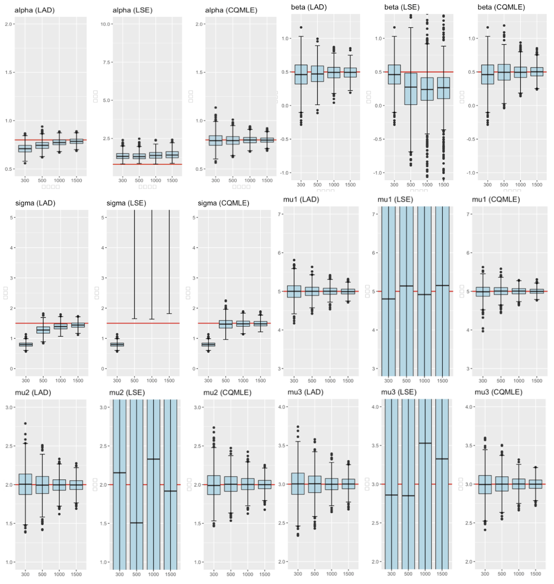
Figure 1. Boxplots of the initial estimators for $n=300,~{}500,~{}1000,~{}1500$ when the true value is $(\alpha,\beta,\sigma,\mu)=(0.8,0.5,1.5,(5,2,3))$; in each panel, the red line shows the true value.

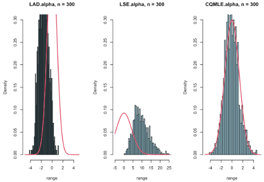
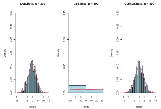
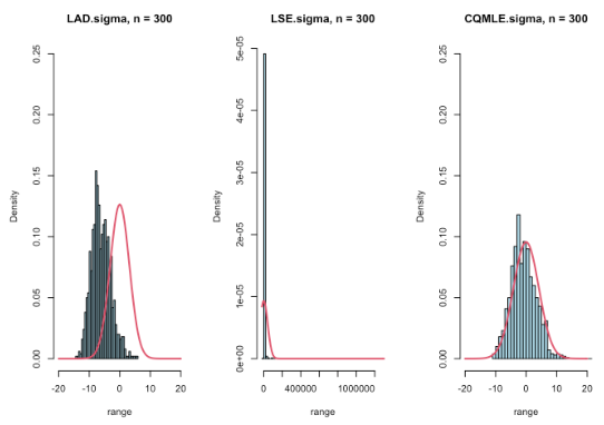
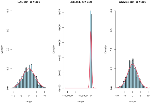
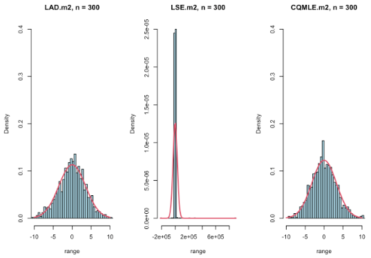
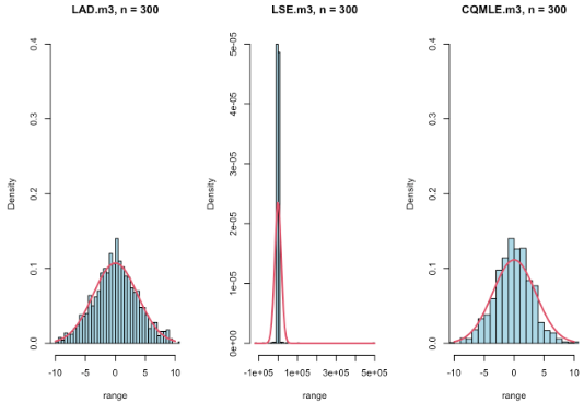
Figure 2. Histograms of the initial estimators for $n=300$ when the true value is $(\alpha,\beta,\sigma,\mu)=(0.8,0.5,1.5,(5,2,3))$; in each panel, the red line represents the probability density function of the normal distribution with the mean 0 and the variance equal to that of the normalized estimator.

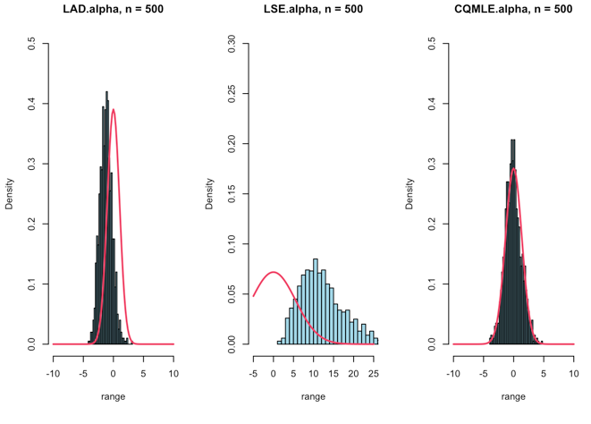
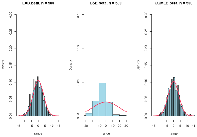
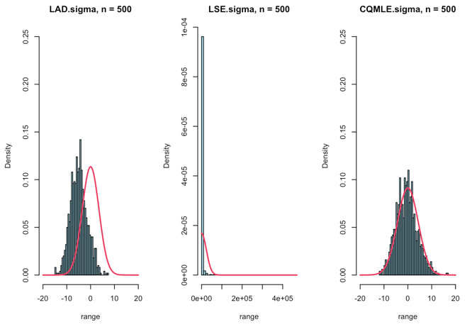
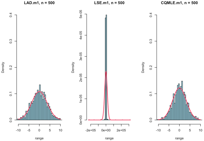
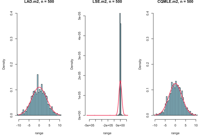
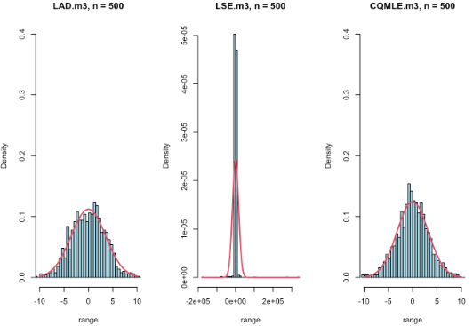
Figure 3. Histograms of the initial estimators for $n=500$ when the true value is $(\alpha,\beta,\sigma,\mu)=(0.8,0.5,1.5,(5,2,3))$; in each panel, the red line represents the probability density function of the normal distribution with the mean 0 and the variance equal to that of the normalized estimator.

Figure 4. Boxplots of the initial estimators for $n=300,500,1000,1500$ when the true value is $(\alpha,\beta,\sigma,\mu)=(1.0,0.5,1.5,(5,2,3))$; in each panel, the red line represents the true value.

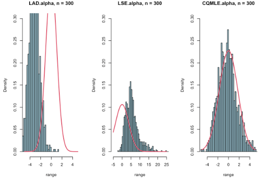
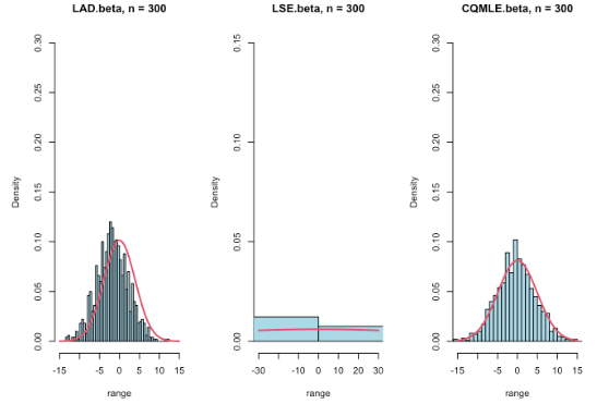
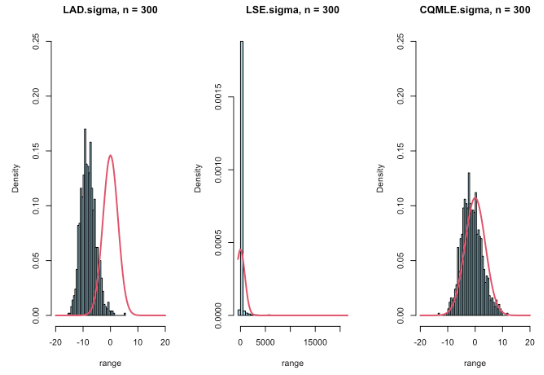
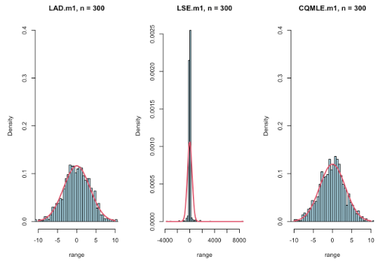
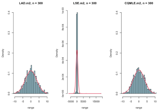
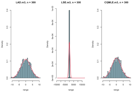
Figure 5. Histograms of the initial estimators for $n=300$ when the true value is $(\alpha,\beta,\sigma,\mu)=(1.0,0.5,1.5,(5,2,3))$; in each panel, the red line represents the probability density function of the normal distribution with the mean 0 and the variance equal to that of the normalized estimator.

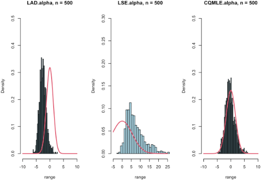
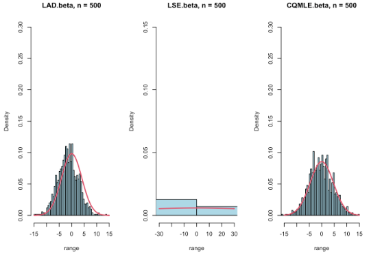
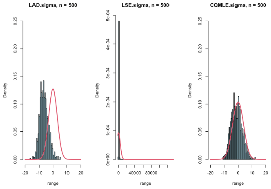
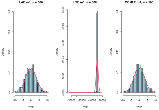
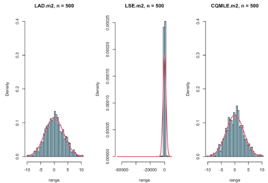
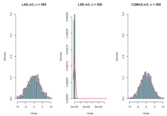
Figure 6. Histograms of the initial estimators for $n=500$ when the true value is $(\alpha,\beta,\sigma,\mu)=(1.0,0.5,1.5,(5,2,3))$; in each panel, the red line represents the probability density function of the normal distribution with the mean 0 and the variance equal to that of the normalized estimator.

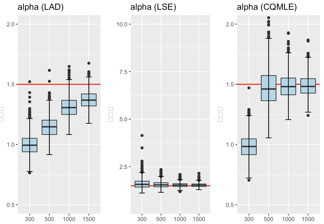
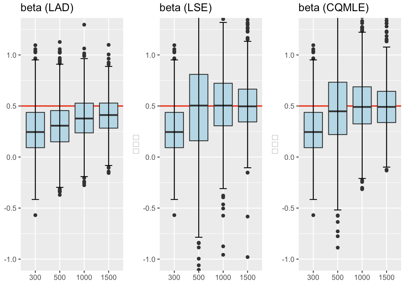
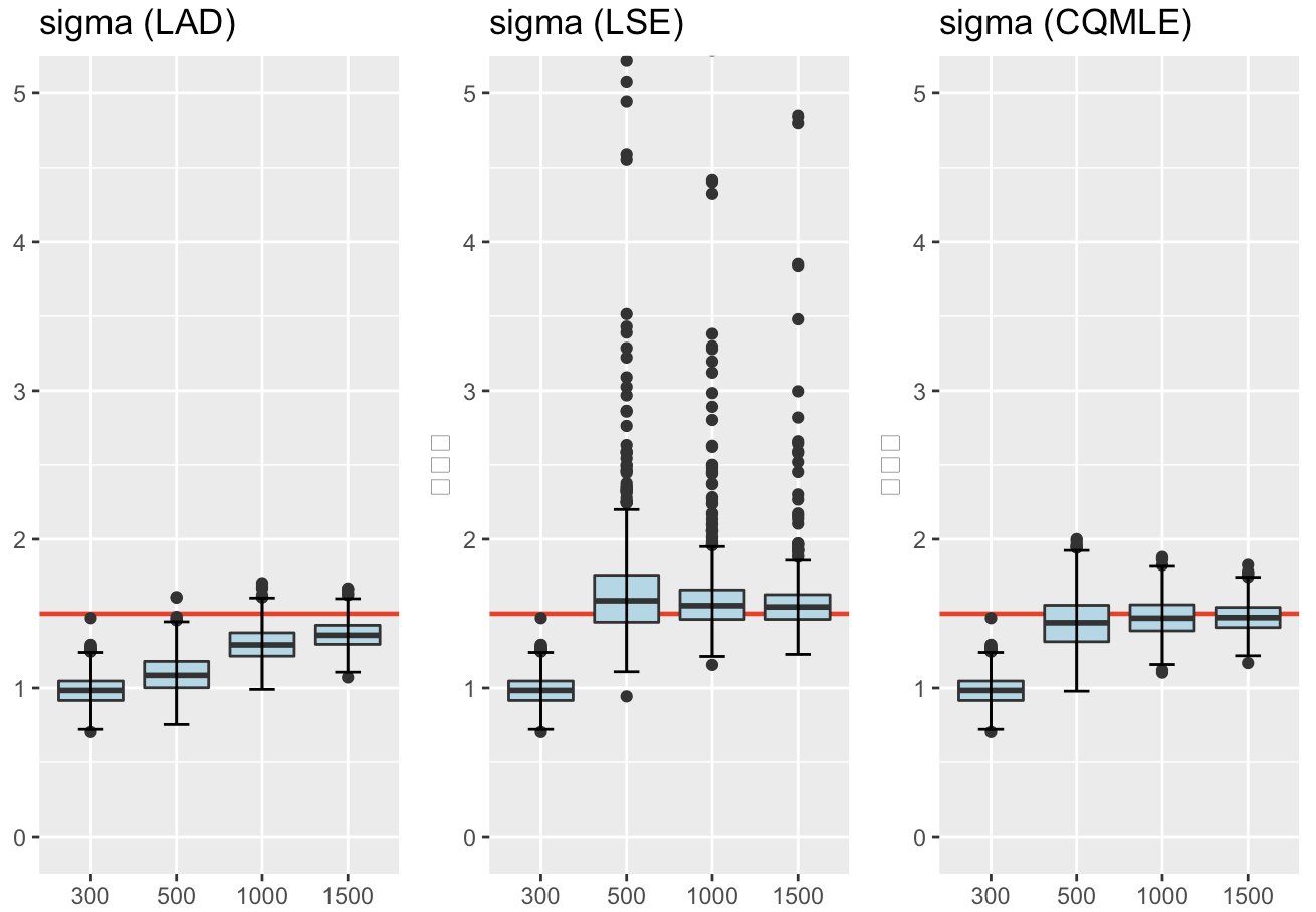
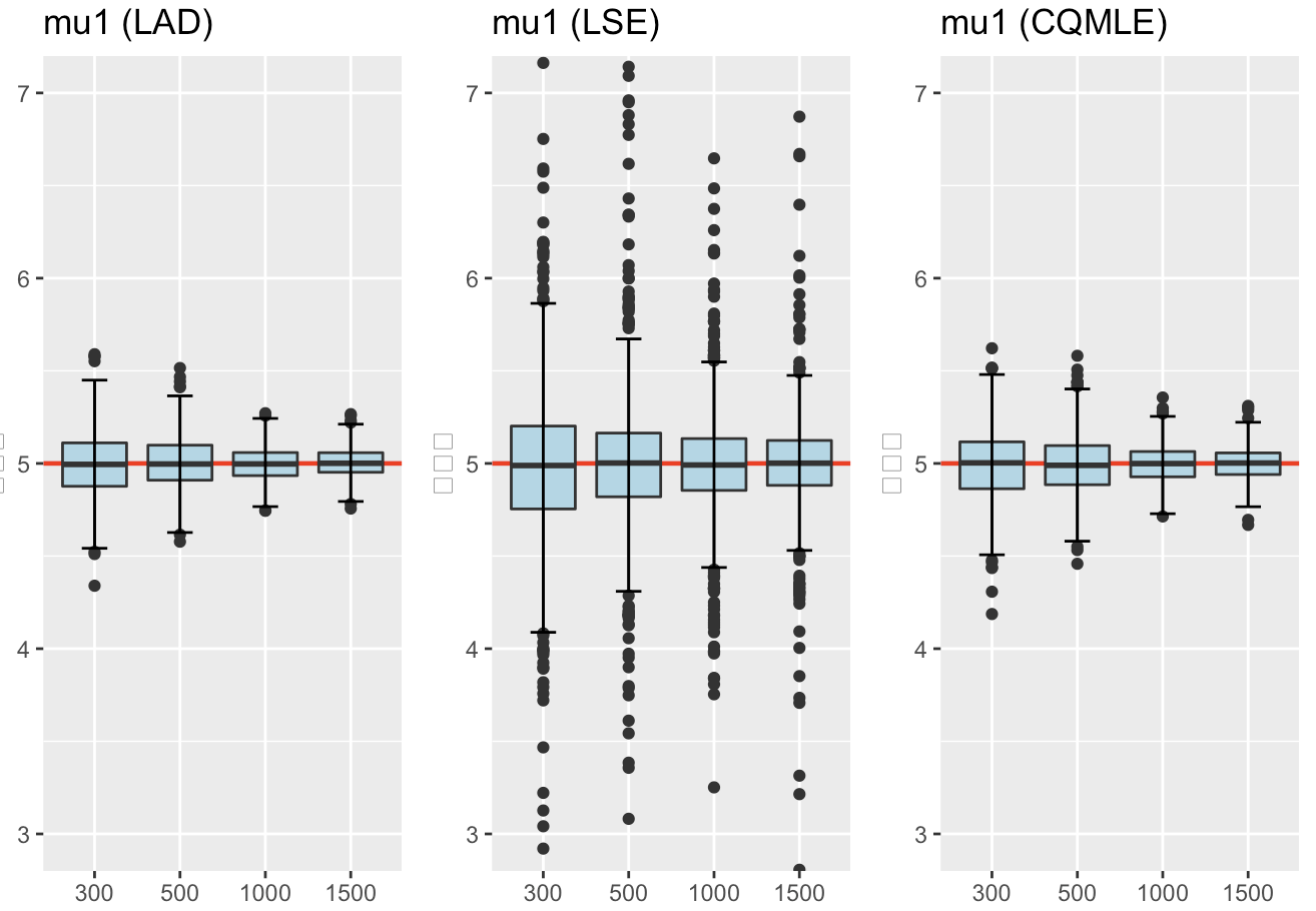
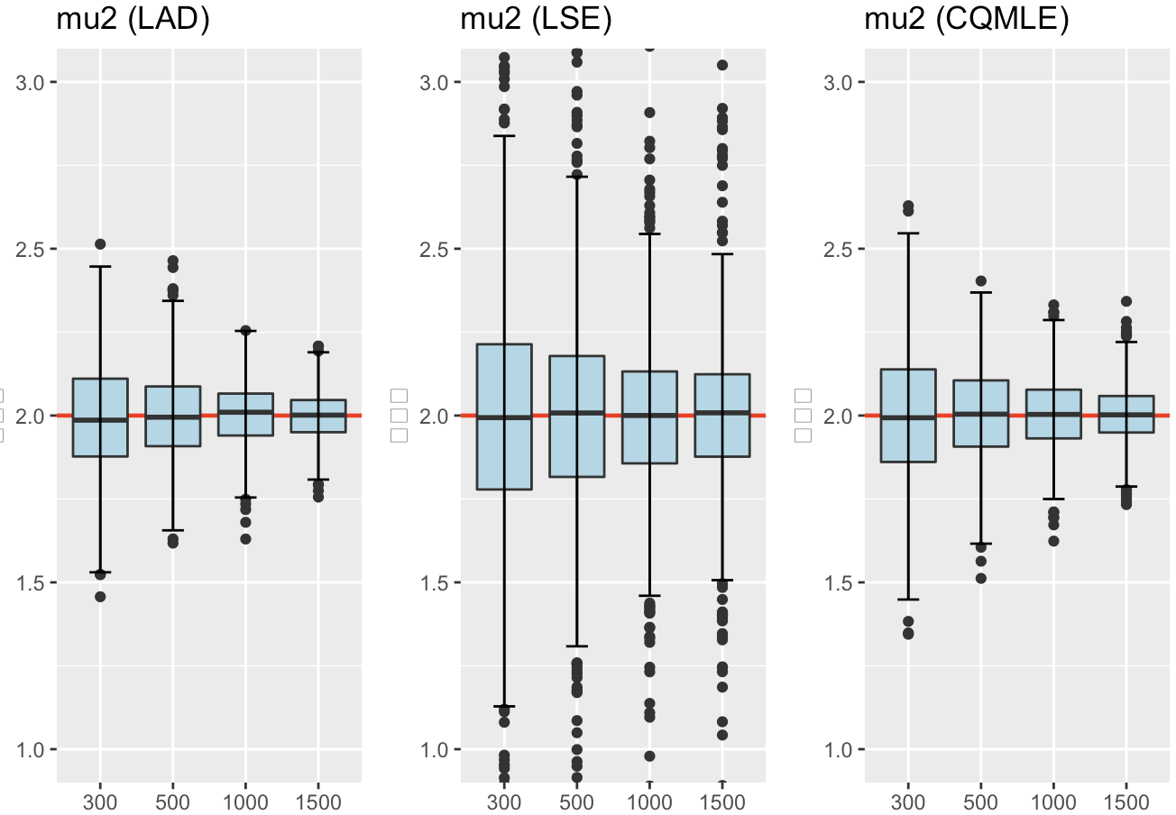
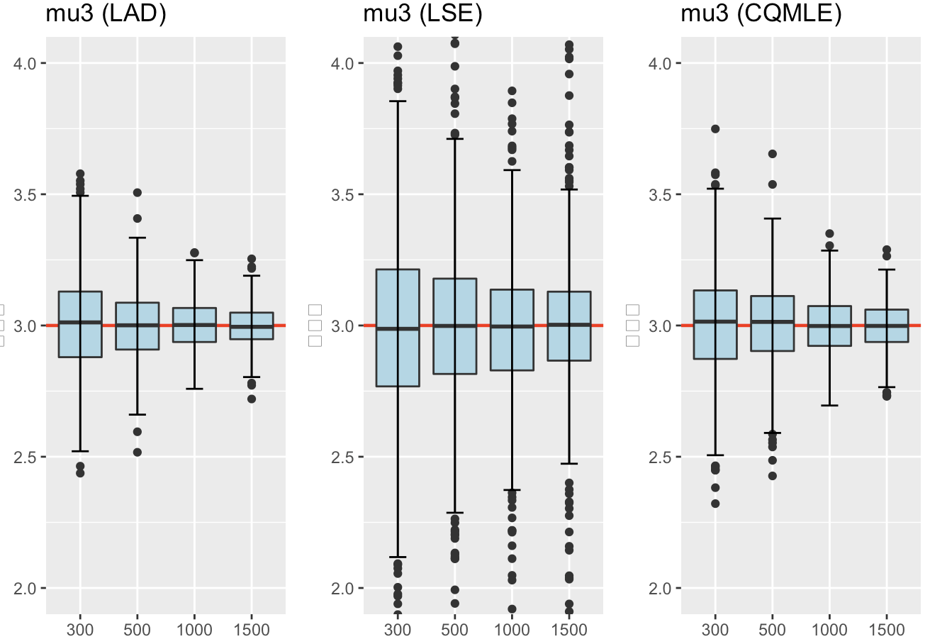
Figure 7. Boxplots of the initial estimators for $n=300,~{}500,~{}1000,~{}1500$ when the true value is $(\alpha,\beta,\sigma,\mu)=(1.5,0.5,1.5,(5,2,3))$; in each panel, the red line shows the true value.

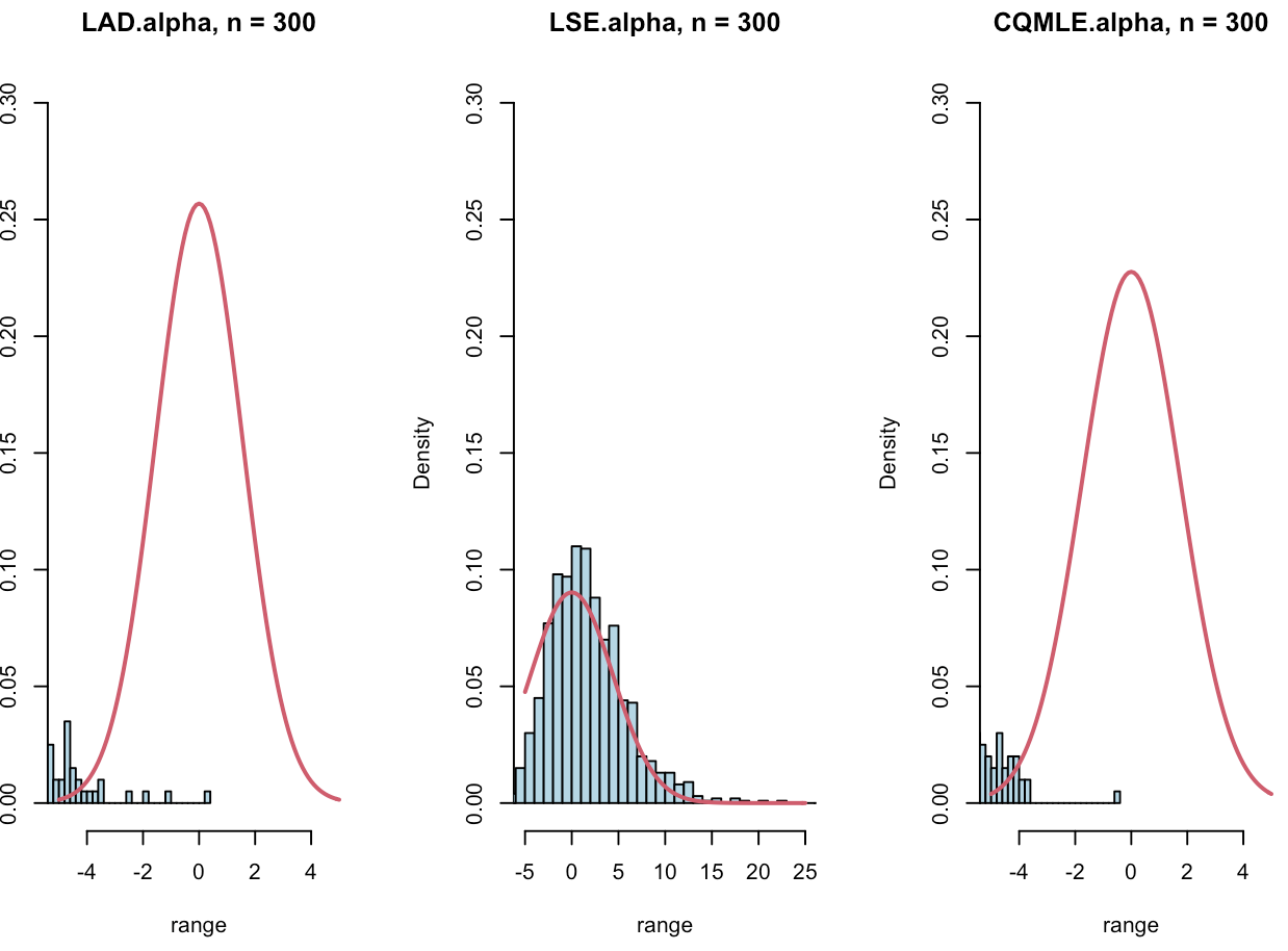
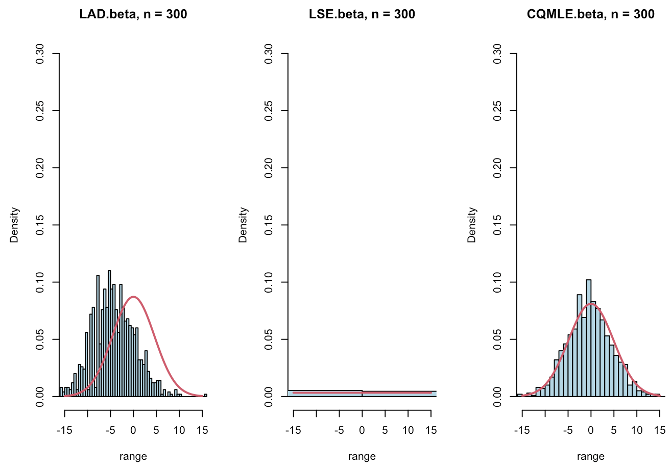
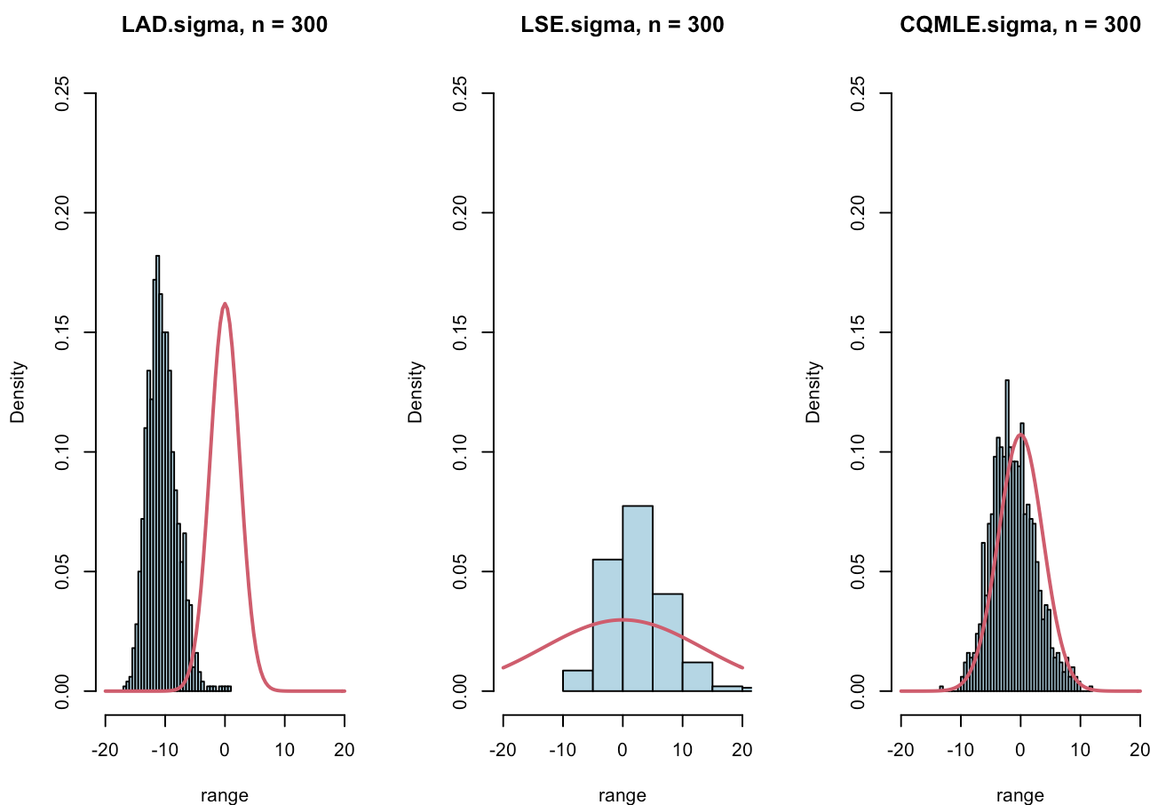
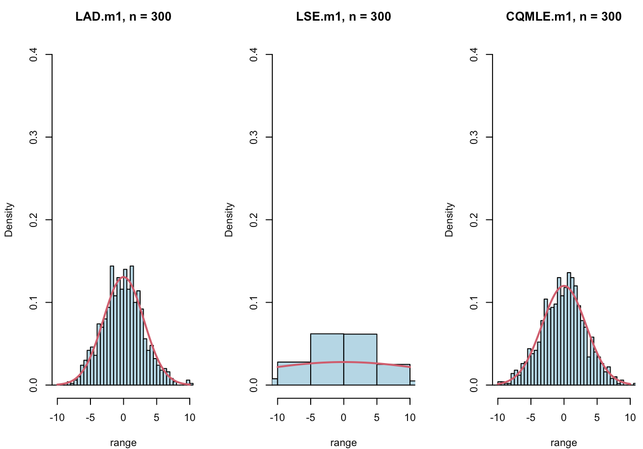
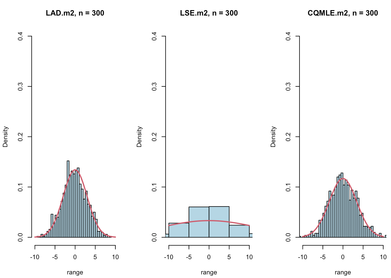
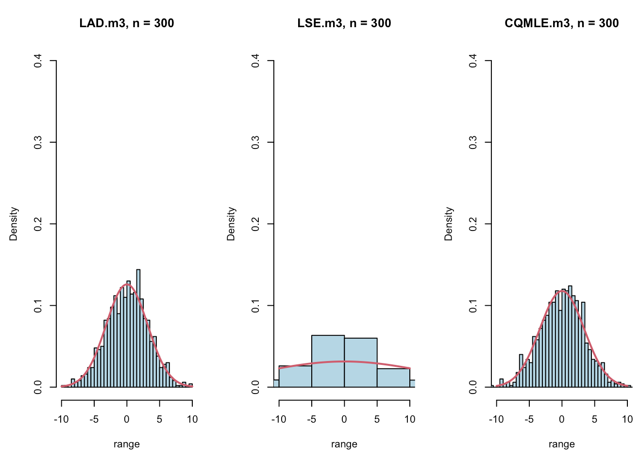
Figure 8. Histograms of the initial estimators for $n=300$ when the true value is $(\alpha,\beta,\sigma,\mu)=(1.5,0.5,1.5,(5,2,3))$; in each panel, the red line represents the probability density function of the normal distribution with the mean 0 and the variance equal to that of the normalized estimator.

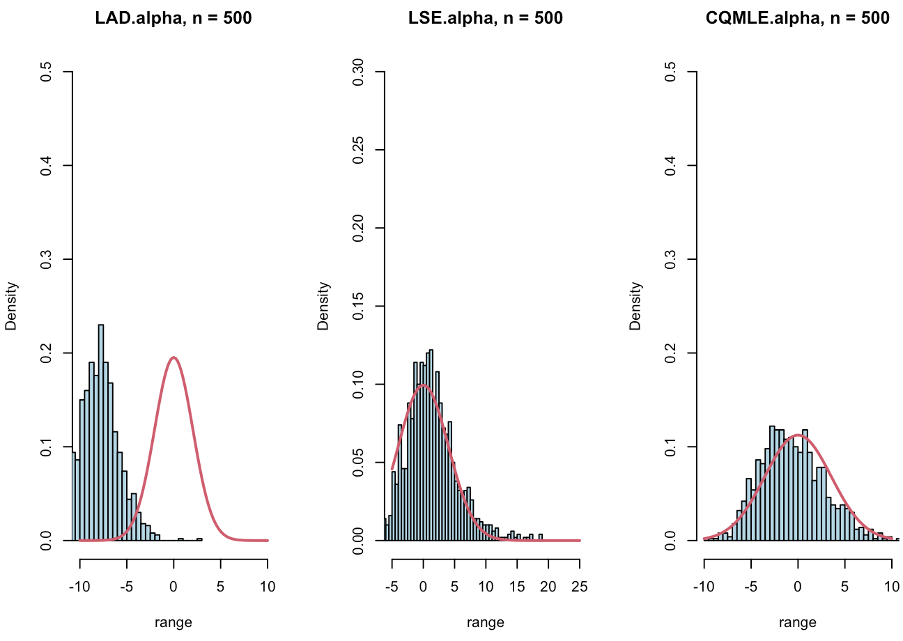
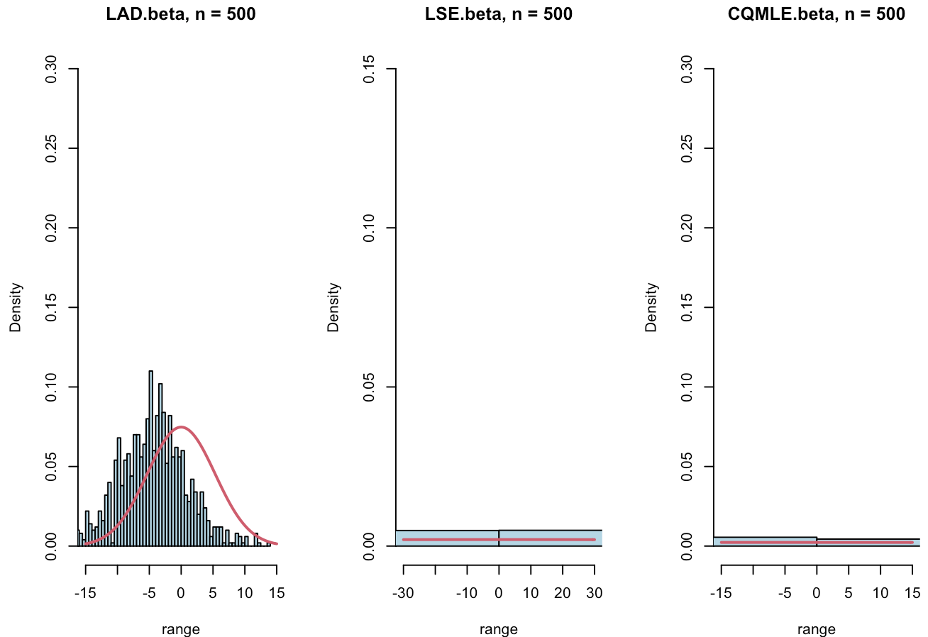
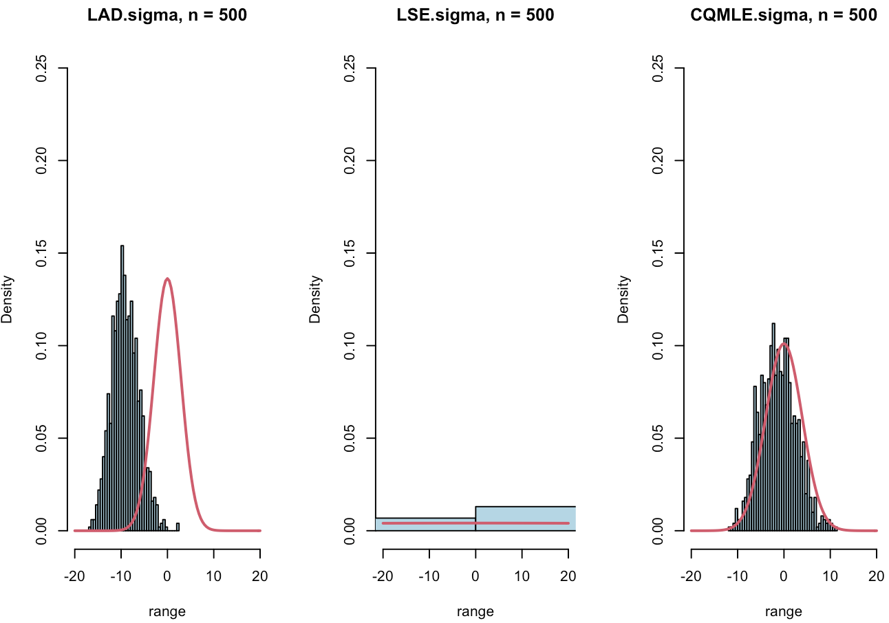
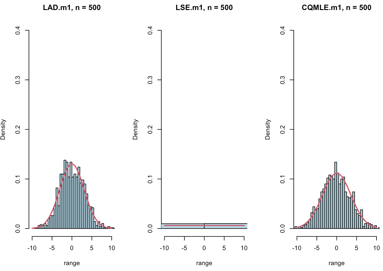
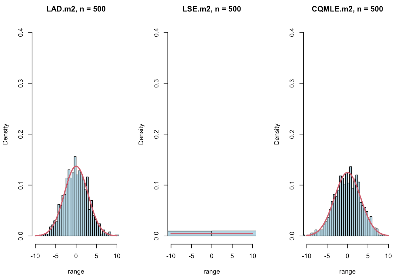
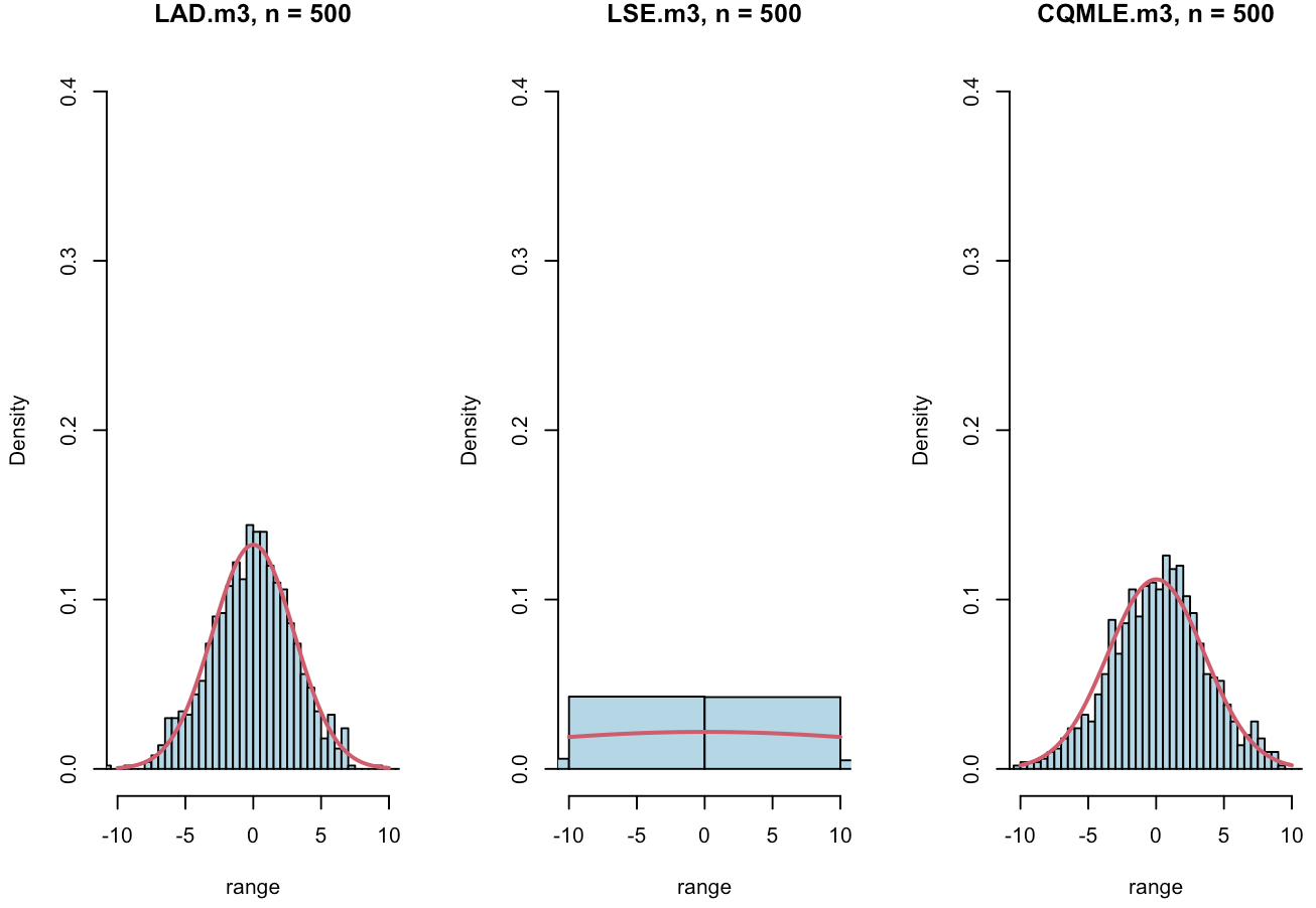
Figure 9. Histograms of the initial estimators for $n=500$ when the true value is $(\alpha,\beta,\sigma,\mu)=(1.5,0.5,1.5,(5,2,3))$; in each panel, the red line represents the probability density function of the normal distribution with the mean 0 and the variance equal to that of the normalized estimator.

4.2. MLE with CQMLE-based initial value

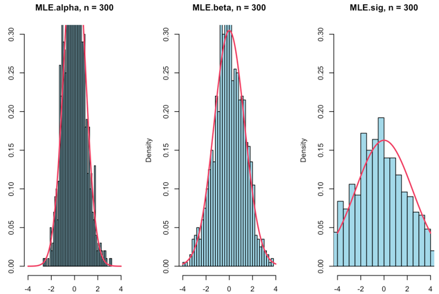
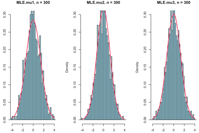
Figure 10. Histograms of the MLE for $n=300$ when we use the true value $(\alpha,\beta,\sigma,\mu)=(0.8,0.5,1.0,(5,2,3))$. The initial value of optimization is the initial estimator when we use CQMLE

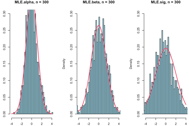
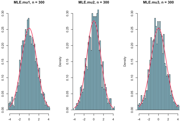
Figure 11. Histograms of the MLE for $n=300$ when we use the true value $(\alpha,\beta,\sigma,\mu)=(1.0,0.5,1.0,(5,2,3))$. The initial value of optimization is the initial estimator when we use CQMLE

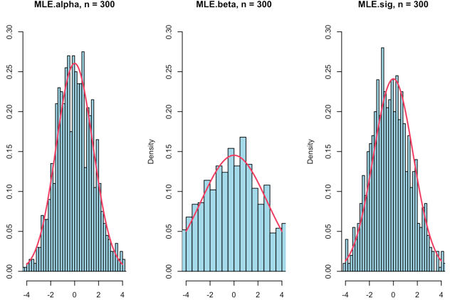
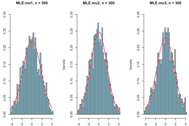
Figure 12. Histograms of the MLE for $n=300$ when we use the true value $(\alpha,\beta,\sigma,\mu)=(1.5,0.5,1.0,(5,2,3))$. The initial value of optimization is the initial estimator when we use CQMLE

Histograms show that the MLE with the CQMLE as an initial estimate for numerical search has good performance for each true value, in particular free from the local-optimum problem.

Acknowledgements. The first author (EK) would like to thank JGMI of Kyushu University for their support. This work was partially supported by JST CREST Grant Number JPMJCR2115 and JSPS KAKENHI Grant Number 22H01139, Japan (HM).

References

• [1] R.ย A. Adams. Some integral inequalities with applications to the imbedding of sobolev spaces defined over irregular domains. Transactions of the American Mathematical Society, 178(0):401โ€“429, 1973.
• [2] B.ย Andrews, M.ย Calder, and R.ย A. Davis. Maximum likelihood estimation for $\alpha$-stable autoregressive processes. Ann. Statist., 37(4):1946โ€“1982, 2009.
• [3] A.ย Dvoretzky. Asymptotic normality for sums of dependent random variables. In Proceedings of the Sixth Berkeley Symposium on Mathematical Statistics and Probability (Univ. California, Berkeley, Calif., 1970/1971), Vol. II: Probability theory, pages 513โ€“535. Univ. California Press, Berkeley, Calif., 1972.
• [4] T.ย S. Ferguson. A course in large sample theory. Texts in Statistical Science Series. Chapman & Hall, London, 1996.
• [5] Y.ย Hosokawa. Estimation of infinite-variance linear regression model. Masterโ€™s thesis, Kyushu University, 2022.
• [6] E.ย E. KuruoฤŸlu. Density parameter estimation of skewed $\alpha$-stable distributions. IEEE Trans. Signal Process., 49(10):2192โ€“2201, 2001.
• [7] M.ย Matsui. Asymptotics of maximum likelihood estimation for stable law with continuous parameterization. Comm. Statist. Theory Methods, 50(15):3695โ€“3712, 2021.
• [8] C.ย L. Nikias and M.ย Shao. Signal processing with alpha-stable distributions and applications. Wiley-Interscience, 1995.
• [9] J.ย P. Nolan. Parameterizations and modes of stable distributions. Statist. Probab. Lett., 38(2):187โ€“195, 1998.
• [10] J.ย P. Nolan. Univariate stable distributions. Springer Series in Operations Research and Financial Engineering. Springer, Cham, [2020] ยฉ2020. Models for heavy tailed data.
• [11] K.-i. Sato. Lรฉvy processes and infinitely divisible distributions, volumeย 68 of Cambridge Studies in Advanced Mathematics. Cambridge University Press, Cambridge, 1999. Translated from the 1990 Japanese original, Revised by the author.
• [12] M.ย Sharpe. Zeroes of infinitely divisible densities. Ann. Math. Statist., 40:1503โ€“1505, 1969.
• [13] A.ย W. vanย der Vaart. Asymptotic statistics, volumeย 3 of Cambridge Series in Statistical and Probabilistic Mathematics. Cambridge University Press, Cambridge, 1998.
• [14] N.ย Yoshida. Polynomial type large deviation inequalities and quasi-likelihood analysis for stochastic differential equations. Ann. Inst. Statist. Math., 63(3):431โ€“479, 2011.
• [15] S.ย Zacks. The theory of statistical inference. John Wiley & Sons, Inc., New York-London-Sydney, 1971. Wiley Series in Probability and Mathematical Statistics.