Consensus-based algorithms for stochastic optimization problems

Abstract

We address an optimization problem where the cost function is the expectation of a random mapping. To tackle the problem two approaches based on the approximation of the objective function by consensus-based particle optimization methods on the search space are developed. The resulting methods are mathematically analyzed using a mean-field approximation and their connection is established. Several numerical experiments show the validity of the proposed algorithms and investigate their rates of convergence.

Keywords: mean-field limit, particle swarm optimization, random optimization problems

MSC2000: 82B40, 65K10, 60K35

1 Introduction

The interest in addressing optimization problems that accommodate for uncertainties has risen in the last decade [20]. When considering optimization problems under uncertain information, there are mainly two choices to be made [5]: first, the way to formalize the variability and, second, the time the uncertain information is revealed with respect to the decision-making. In this manuscript we restrict to the class of static stochastic optimization problems (sSOPs ), namely to minimization tasks where the uncertain information is described by means of random variables and where the optimization effort is applied before the random event has taken place. More precisely, we consider problems of the type:

$$\min_{x\in\mathbb{R}^{d}}\{f(x):=\mathbb{E}_{\mathbb{P}}[F(x,\mathbf{Y})]\}.$$ (1)

Here $d\geq 1$, $\mathbf{Y}$ is a random variable defined on the probability space $(\Omega,\mathcal{A},\mathbb{P})$ and it is supported on a set $E\subset\mathbb{R}^{k},k\geq 1$, with law $\nu^{\mathbf{Y}}$. Further, $F:\mathbb{R}^{d}\times E\to\mathbb{R}$ is some nonlinear, non-convex objective function. $\mathbb{E}_{\mathbb{P}}$ denotes the mathematical expectation with respect to $\mathbb{P}$, that is, for any $x\in\mathbb{R}^{d}$,

$$\mathbb{E}_{\mathbb{P}}[F(x,\mathbf{Y})]=\int_{\Omega}F(x,\mathbf{Y}(\omega))d\mathbb{P}(\omega)=\int_{E}F(x,\mathbf{y})d\nu^{\mathbf{Y}}(\mathbf{y}).$$

In the manuscript, we will assume that $\mathbf{y}\mapsto F(x,\mathbf{y})$ is measurable for all $x$ and positive, $\mathbb{E}_{\mathbb{P}}[F(x,\mathbf{Y})]$ is finite for all $x\in\mathbb{R}^{d}$, i.e.,

$$F(x,\cdot)\in L^{1}(\Omega,\mathcal{A},\mathbb{P})\quad\textnormal{or}\quad F(x,\cdot)\in L^{1}_{\nu^{\mathbf{Y}}}(E,\mathcal{B}(E)),\quad\textnormal{resp.}$$

Here, $\mathcal{B}(E)$ is the Borel set of $E$. In addition, we require that $f:\mathbb{R}^{d}\to\mathbb{R}$ admits a global minimizer $x_{\star}\in\mathbb{R}^{d}$.

Among the approaches for solving (1), we are interested in meta-heuristics in order to treat possibly non-differentiable and non-convex functions $F$. These are exploring the search space by balancing the exploitation of the accumulated search experience and exploration [7, 5]. Some notable examples include Ant Colony Optimization, Genetic Algorithms, Particle Swarm Optimization, Consensus-Based Optimization and Simulated Annealing. The growth of interest in such procedures has been a result of their ability of finding a nearly optimal solution for problem instances of realistic size in a generally reasonable computation time, see e.g. [30, 29, 4]. Despite this benefit, most of these methods lack a formal mathematical justification for their efficiency.

Recent progress in this direction has been made for the class of Consensus-Based Optimization (CBO) algorithms being amenable to theoretical analysis via tools from statistical physics [42, 15, 16, 23, 24]. These methods use a set of $N\in\mathbb{N}$ particles to explore the domain and find a global minimum of the objective function $f$. The dynamics of the agents is governed by a drift term that drags them towards a momentaneous consensus point (that serves as a temporary guess for $x_{\star}$) and a diffusion term, that favors the exploration of the search space. Due to the derivative-free nature of the CBO algorithms, they are applied to (non-convex) non-smooth functions; furthermore, several variations of such methods have been proposed to accommodate for the presence of constraints [11, 17, 22, 25], multiple objectives [9, 10] and multiple minimizers [26].
The theoretical analysis of the CBO methods may be conducted at the algorithmic (hereafter called microscopic) level, as done for instance in [31, 32, 39], or at the mean-field level [8] where a statistical description of the dynamics of the average agent behavior is considered. In the following we adopt the latter viewpoint as in [23].

In this manuscript, we develop two approaches for tackling problem (1). Common to both methods is the approximation of the true objective function $f$ by a suitable sampling and the resolution of the newly obtained problem with the designated CBO algorithm. The first approach is based on the Sample Average Approximation (SAA) [43, 44] and it consists of substituting $f$ with a Monte-Carlo estimator $\hat{f}_{M}$ that depends on a sample $(\mathbf{y}^{(1)},\ldots,\mathbf{y}^{(M)})^{T}\in E^{M}$ of $M$ realizations of the random vector $\mathbf{Y}$. For $M$ large, $\hat{f}_{M}\approx f$ and it is a matter of simple calculations to derive the mean-field equation associated to the microscopic system by letting first $M\to\infty$ and then letting $N\to\infty$. However, it is not clear a priori, if the same equation is obtained by performing the limits in the opposite order: in this paper we investigate this question and prove, under additional assumptions, that the answer is positive, see Figure 1 (outer loop). The second approach (hereafter called quadrature approach) consists of approximating $f$ by a suitable quadrature formula $\tilde{f}_{N}$ with $M=N$ fixed discretization points $(\mathbf{y}_{1},\ldots,\mathbf{y}_{N})^{T}\in E$. We require the number of agents in the algorithm to be equal to the number of nodes $N$: this allows us to consider the dynamics of the agents to take place in the augmented space $\mathbb{R}^{d}\times E$ and to derive the corresponding mean-field equation on the extended phase space. We then prove that this approach yields the same limiting equation up to a scaling factor, see Figure 1 (inner diagonal).

Figure 1: Mean-field formulations of the SAA approach (outer loop) and the quadrature approach (inner diagonal).

The rest of the paper is organized as follows. In Section 2, we illustrate the combination of the SAA approach and of the CBO algorithm. After presenting the algorithm, we give a detailed proof of the arrows of the outer loop of Figure 1. We justify the hypotheses made in view of the key theoretical properties of the solutions obtained through the SAA approach. In Section 3, we present the quadrature approach and, in Section 4, we rigorously prove the equality of the mean-field formulations of the two approaches, hence, demonstrating the diagonal arrow of Figure 1. We devote Section 5 to some numerical tests aiming at investigating the rates of the SAA and quadrature approach and at comparing the two methods. We summarize our main conclusions in Section 6 and provide an overview of possible directions for further research.

2 The sample average approximation approach

A common approach for tackling global optimization problem (1) is the Sample Average Approximation (SAA) approach (see e.g. [43, 44]). It consists of three steps:

1. sample $\mathbf{Y}^{(1)},\ldots,\mathbf{Y}^{(M)}$ from the random vector $\mathbf{Y}$, for a fixed $M>0$;

2. approximate $f(x)=\mathbb{E}_{\mathbb{P}}[F(x,\mathbf{Y})]$ with the so-called Sample Average Approximation (SAA)

   $$\hat{f}_{M}(x):=\frac{1}{M}\sum_{j=1}^{M}F(x,\mathbf{Y}^{(j)})\quad\textnormal{for}\;x\in\mathbb{R}^{d};$$ (2)

3. solve the optimization problem

   $$\min_{x\in\mathbb{R}^{d}}\hat{f}_{M}(x).$$ (3)

We remark that the sample drawn from $\mathbf{Y}$ can be either a sequence of random vectors (we will denote this with uppercase letters $\mathbf{Y}^{(1)},\ldots,\mathbf{Y}^{(M)}$) or a particular realization of that sequence (we will denote this with lowercase letters $\mathbf{y}^{(1)},\ldots,\mathbf{y}^{(M)}$). In addition, we remark that when the sample is treated as a sequence of random vectors the function $\hat{f}_{M}$ depends on the particular realization $\omega\in\Omega$. With abuse of notation, we use the representation of $\hat{f}_{M}$ as a function of $x$ and as a function of $x$ and $\omega$.

In the following, we apply a CBO-type algorithm to solve deterministic problem (3). We consider a stochastic system of $N\in\mathbb{N}$ agents with position vectors $X^{i}_{t}\in\mathbb{R}^{d},i=1,\ldots,N$, that dynamically interact with each other to find the minimizer of the objective function. More precisely, the CBO update rule is given, at time $t\geq 0$, by the system of SDEs

$$dX^{i}_{t} =-\lambda(X^{i}_{t}-x^{\alpha,M}_{t})dt+\sigma D^{i}_{t}dB^{i}_{t}\quad\textnormal{for}\;i=1,\ldots,N,$$ (4a)

$$x^{\alpha,M}_{t} =\frac{\sum_{i=1}^{N}X^{i}_{t}\exp(-\alpha\hat{f}_{M}(X^{i}_{t}))}{\sum_{i=1}^{N}\exp(-\alpha\hat{f}_{M}(X^{i}_{t}))},$$ (4b)

where $\lambda,\sigma>0$, $\alpha>0$, and $B^{i}_{t}$ are $d$-dimensional independent Brownian processes. In system (4a) the drift term is governed by $\lambda$, moving particles towards the consensus point $x^{\alpha,M}_{t}$, and the diffusion term is governed by $\sigma$, for exploration in the search space. $D^{i}_{t}$ is a matrix in $\mathbb{R}^{d\times d}$ that can be chosen either as

$$D^{i}_{t}=D^{i}_{t,\textnormal{iso}}:=|X^{i}_{t}-x^{\alpha,M}_{t}|I_{d},\quad\textnormal{where $I_{d}\in\mathbb{R}^{d\times d}$ is the identity matrix},$$

so that the random exploration process is isotropic [42] and all dimensions $l=1,\ldots,d$ are equally explored, or as

$$D^{i}_{t}=D^{i}_{t,\textnormal{aniso}}:=\textnormal{diag}(X^{i}_{t}-x^{\alpha,M}_{t}),$$

so that it is anisotropic [16]. In the following, we fix $D^{i}_{t}=D^{i}_{t,\textnormal{aniso}}$ for clarity of exposition. The exponential coefficients in the weighted average $x^{\alpha,M}_{t}$ (4b) fulfill

$$x^{\alpha,M}_{t}\xrightarrow[]{\alpha\to\infty}\textnormal{argmin}_{i=1,\ldots,N}\hat{f}_{M}(X^{i}_{t}).$$

The above convergence is guaranteed by the Laplace principle [21], see also [42, 15, 16, 23, 24]. The system is supplemented with initial conditions $X^{i}_{0},i=1,\ldots,N$, independent and identically distributed (i.i.d.) with law $\mu_{0}\in\mathcal{P}(\mathbb{R}^{d})$.

For a fixed $\omega\in\Omega$, $\hat{f}_{M}$ is a deterministic function that depends on $\mathbf{y}=(\mathbf{y}^{(1)},\ldots,\mathbf{y}^{(M)})^{T}$: therefore, $\mathbf{y}$ may be thought of as a parameter and the analytical results of the CBO theory can be transferred to system (4) provided that $\hat{f}_{M}$ satisfies the corresponding assumptions [16, 23]. If $\mathbb{E}[|(X^{1}_{0},\ldots,X^{N}_{0})|^{2}]<\infty$ and $F$ is locally Lipschitz continuous in the first variable and uniformly in the second, then the microscopic algorithm (4) is well-posed.

2.1 The mean-field equation for $M\to\infty$, then $N\to\infty$

Consider the CBO algorithm (4) and let $N$ and $t$ be fixed. We remark that such system of SDEs depends on $M$ only through the weighted average $x^{\alpha,M}_{t}$ (4b). Therefore, evaluating the limit as $M\to\infty$ of the dynamics (4) reduces to determining the limit as $M\to\infty$ of $x^{\alpha,M}_{t}$. In the following, we treat $\mathbf{Y}^{(1)},\ldots,\mathbf{Y}^{(M)}$ (and consequently the corresponding consensus points $\{x^{\alpha,M}_{t}\}_{M}$) as random vectors and intend the limit for $M\to\infty$ in the almost sure (a.s.) convergence sense.

Let’s assume that

Assumption 2.1.

The sample $\left\{\mathbf{Y}^{(j)}\right\}_{j=1,\ldots,M}$ is independent and identically distributed (i.i.d.) with law $\nu^{\mathbf{Y}}$.

Then, the measurability of $F$ in the second component and a direct application of the point-wise law of large numbers, see e.g. [6], imply for any $x\in\mathbb{R}^{d}$

$$\hat{f}_{M}(x)=\frac{1}{M}\sum_{j=1}^{N}F(x,\mathbf{Y}^{(j)})\xrightarrow[M\to\infty]{\textnormal{a.s.}}\mathbb{E}_{\mathbb{P}}[F(x,\mathbf{Y})]=f(x).$$

Thanks to the continuous mapping theorem (see again e.g. [6]), we obtain that

$$x^{\alpha,M}_{t}=\frac{\sum_{i=1}^{N}X^{i}_{t}\exp(-\alpha\hat{f}_{M}(X^{i}_{t}))}{\sum_{i=1}^{N}\exp(-\alpha\hat{f}_{M}(X^{i}_{t}))}\xrightarrow[M\to\infty]{\textnormal{a.s.}}\frac{\sum_{i=1}^{N}X^{i}_{t}\exp(-\alpha f(X^{i}_{t}))}{\sum_{i=1}^{N}\exp(-\alpha f(X^{i}_{t}))}.$$

We denote by $x^{\alpha,f}_{t}\in\mathbb{R}^{d}$ the limit value obtained above. To summarize, we have shown that, for a fixed $N$, the CBO algorithm (4) converges, as $M\to\infty$, to the system

$$dX^{i}_{t} =-\lambda(X^{i}_{t}-x^{\alpha,f}_{t})dt+\sigma\textnormal{diag}(X^{i}_{t}-x^{\alpha,f}_{t})dB^{i}_{t}\quad\textnormal{for}\;i=1,\ldots,N,$$ (5a)

$$x^{\alpha,f}_{t} =\quad\frac{\sum_{i=1}^{N}X^{i}_{t}\exp(-\alpha f(X^{i}_{t}))}{\sum_{i=1}^{N}\exp(-\alpha f(X^{i}_{t}))},$$ (5b)

which is again a CBO algorithm with consensus point given by $x^{\alpha,f}_{t}$ (5b).

Similarly to the previous works on the CBO, we formallly derive the mean-field equation associated to (5) by using the propagation of chaos assumption on the marginals [18, 28, 36].For fixed time $t$, let $H^{N}(t)$ be the $N$-particle probability distribution over $(\mathbb{R}^{d})^{N}$ at time $t$. Then, the assumption translates to $H^{N}(t)=h(t)^{\otimes N}$ for a probability distribution $h(t)$ over $\mathbb{R}^{d}$. Finally, we obtain that $h$ satisfies in the distributional sense

$$\partial_{t}h(t,x) =\lambda\nabla_{x}\cdot\left((x-\bar{x}^{\alpha,f}_{t})\>h(t,x)\right)+\frac{\sigma^{2}}{2}\sum_{l=1}^{d}\frac{\partial^{2}}{\partial x_{l}^{2}}\left((x-\bar{x}^{\alpha,f}_{t})^{2}_{l}\>h(t,x)\right)$$ (6a)

$$\bar{x}^{\alpha,f}_{t} =\frac{\int_{\mathbb{R}^{d}}x\exp(-\alpha f(x))h(t,x)dx}{\int_{\mathbb{R}^{d}}\exp(-\alpha f(x))h(t,x)dx},$$ (6b)

$$\mu_{0}(dx) =\lim_{t\to 0}h(t,x)dx.$$ (6c)

A rigorous proof of the well-posedness of the weak formulation of (6), as well as the conclusion that $h(t,x)dx\in\mathcal{P}_{2}(\mathbb{R}^{d})$ , is given in [42, 15] under the hypotheses that $\mu_{0}\in\mathcal{P}_{4}(\mathbb{R}^{d})$ and that $f$ is bounded and satisfies suitable growth conditions. We also note that the above formal derivation may be made rigorous by proceeding as in [35].

We have proven the following result.

Lemma 2.1.

Let $\left\{\mathbf{Y}^{(j)}\right\}_{j=1,\ldots,M}$ satisfy Assumption 2.1. Then,

2.2 The mean-field equation for $N\to\infty$, then $M\to\infty$

We investigate if the mean-field formulation (6) is obtained by the CBO algorithm (4) by considering the limit for $N\to\infty$ and then $M\to\infty$. The section provides a positive answer, under additional assumptions on the consistency with the classical theory of SAA.

Let $M$ be fixed. Proceeding as in the previous section, we obtain, in the regime of the large number of particles ($N\to\infty$), the mean-field formulation associated to (4):

$$\partial_{t}\tilde{h}(t,x) =\lambda\nabla_{x}\cdot\left((x-\bar{x}^{\alpha,M}_{t})\>\tilde{h}(t,x)\right)+\frac{\sigma^{2}}{2}\sum_{l=1}^{d}\frac{\partial^{2}}{\partial x_{l}^{2}}\left((x-\bar{x}^{\alpha,M}_{t})^{2}_{l}\>\tilde{h}(t,x)\right),\quad\textnormal{for $x\in\mathbb{R}^{d}$,}$$ (7a)

$$\bar{x}^{\alpha,M}_{t} =\frac{\int_{\mathbb{R}^{d}}x\exp(-\alpha\hat{f}_{M}(x))\tilde{h}(t,x)dx}{\int_{\mathbb{R}^{d}}\exp(-\alpha\hat{f}_{M}(x))\tilde{h}(t,x)dx},$$ (7b)

$$\mu_{0}(dx) =\lim_{t\to 0}\tilde{h}(t,x)dx.$$ (7c)

In the rest of the section we will denote the dependence of the consensus point on the mean-field distribution $\tilde{h}$ by $\bar{x}^{\alpha,M}_{t}=\bar{x}^{\alpha,M}_{t}[\tilde{h}]$.

Adopting the same argument of the previous section, we investigate the limit as $M\to\infty$ of $\bar{x}^{\alpha,M}_{t}[\tilde{h}]$. We preface the following uniform law of large numbers, key ingredient in our reasoning.

Theorem 2.1 ([44], Theorem 7.48 (ULLN)).

Assume that $\left\{\mathbf{Y}^{(j)}\right\}_{j=1,\ldots,M}$ satisfy Assumption 2.1 and let $C$ be a nonempty compact subset of $\mathbb{R}^{d}$ such that

1. for any $x\in C$, the function $F(\cdot,\mathbf{y})$ is continuous at $x$ for almost every $\mathbf{y}\in E$;

2. for any $x\in C$, the function $y\mapsto F(x,\mathbf{y})$ is dominated by an integrable function.

Then, $\hat{f}_{M}$ converges to $f$ uniformly on $C$. Namely, there $\exists\;\mathcal{N}\in\mathcal{A}$ a set of measure zero (with respect to probability measure $\mathbb{P}$) such that for any $\omega\in\Omega\setminus\mathcal{N}$

$$\lim_{M\to\infty}\sup_{x\in\mathcal{C}}|\hat{f}_{M}(x,\omega)-f(x)|=0.$$ (8)

We claim that

$$\bar{x}^{\alpha,M}_{t}[\tilde{h}]\;\xrightarrow[M\to\infty]{\textnormal{a.s.}}\;\bar{x}^{\alpha,f}_{t}[\tilde{h}]:=\frac{\int_{\mathbb{R}^{d}}x\exp(-\alpha f(x))\tilde{h}(t,x)dx}{\int_{\mathbb{R}^{d}}\exp(-\alpha f(x))\tilde{h}(t,x)dx},$$

and provide a precise statement of the convergence result in the lemma that follows.

Lemma 2.2.

Assume that $C$ and $F$ are such that the ULLN 2.1 holds and $\textnormal{supp}(\tilde{h}(t,x)dx)\subset C$ for any $t$. Then, there exists $\widetilde{\mathcal{N}}\in\mathcal{A}$ a set of measure zero such that for any $\omega\in\Omega\setminus\widetilde{\mathcal{N}}$

$$\bar{x}^{\alpha,M}_{t}[\tilde{h}](\omega)=\frac{\int_{\mathbb{R}^{d}}x\exp(-\alpha\hat{f}_{M}(x,\omega))\tilde{h}(t,x)dx}{\int_{\mathbb{R}^{d}}\exp(-\alpha\hat{f}_{M}(x,\omega))\tilde{h}(t,x)dx}\;\xrightarrow[M\to\infty]{}\;\frac{\int_{\mathbb{R}^{d}}x\exp(-\alpha f(x))\tilde{h}(t,x)dx}{\int_{\mathbb{R}^{d}}\exp(-\alpha f(x))\tilde{h}(t,x)dx}=\bar{x}^{\alpha,f}_{t}[\tilde{h}](\omega).$$

Proof.

We choose $\widetilde{\mathcal{N}}=\mathcal{N}$ of Theorem 2.1 and fix $\omega\in\Omega\setminus\mathcal{N}$. We start out by proving the convergence of the numerators.

$$\bigg{|}\int_{\mathbb{R}^{d}}x \exp(-\alpha\hat{f}_{M}(x,\omega))-x\exp(-\alpha f(x))\tilde{h}(t,x)dx\bigg{|}$$

$$\hskip 17.07182pt\leq\;\int_{\mathbb{R}^{d}}\left|x\exp(-\alpha\hat{f}_{M}(x,\omega))-x\exp(-\alpha f(x))\right|\tilde{h}(t,x)dx$$

$$\underbrace{=}_{\textnormal{supp}(\tilde{h}(t,x)dx)\subset C}\int_{C}\left|x\exp(-\alpha\hat{f}_{M}(x,\omega))-x\exp(-\alpha f(x))\right|\tilde{h}(t,x)dx$$

$$\hskip 11.38092pt\underbrace{\leq}_{1-\textnormal{Lip}}\int_{C}|x|\left|\hat{f}_{M}(x,\omega)-f(x)\right|\tilde{h}(t,x)dx\leq\underbrace{\sup_{x\in\mathcal{C}}|\hat{f}_{M}(x,\omega)-f(x)|}_{\xrightarrow[M\to\infty]{}0}\underbrace{\int_{C}|x|\tilde{h}(t,x)dx}_{<\infty}$$

where in the second inequality we have used the fact that $z\mapsto e^{-\alpha z}$ is 1-Lipschitz for $z\geq 0$ (and $\hat{f}_{M},f$ can be chosen non negative without loss of generality) and in the third that

$$\int_{C}|x|\tilde{h}(t,x)dx\leq\int_{\mathbb{R}^{d}}|x|\tilde{h}(t,x)dx<\infty$$

thanks to the fact that $\tilde{h}(t,x)dx\in\mathcal{P}_{2}(\mathbb{R}^{d})$ by virtue of the results mentioned at the end of the last subsection.

We proceed in the same way for the denominators and conclude that the result holds in particular for the quotient. ∎

To sum up, we have proven, by taking first the limit for $N\to\infty$ and then $M\to\infty$ in the CBO algorithm (4), that $\tilde{h}$ is a weak solution to the mean-field formulation with consensus point $\bar{x}^{\alpha,f}_{t}[\tilde{h}]$. We would like to state that $\tilde{h}$ “coincides” with $h$, weak solution to (6), or, in other words, that the weak solution of (6) is unique. The uniqueness has already been proven in Lemma 3.2 of [35] in the sense of the $2$-Wasserstein distance and uniformly in time, provided that the two weak solutions share the same initial data. This is fulfilled here since we start out from CBO algorithm (4) with $X^{i}_{0}$ distributed according to $\mu_{0}$.

Merging Lemma 2.1, Lemma 2.2 and the observation done in the previous paragraph, we conclude the following.

Theorem 2.2.

Let $\left\{\mathbf{Y}^{(j)}\right\}_{j=1,\ldots,M}$ satisfy Assumption 2.1. Let $C$ and $F$ be such that the ULLN 2.1 holds and $\textnormal{supp}(h(t,x)dx)\subset C$ for any $t$, with $h$ weak solution to (6). Then, the following diagram holds

In particular, we conclude that (6) is the mean-field formulation associated to system (4), regardless of the order in which we take the limits in $M$ and $N$.

We comment the assumptions made in Theorem 2.2. The request that the ULLN holds is natural in the statistical analysis of the SAA approach. Indeed, in the SAA research a thoroughly investigated question is what are sufficient conditions for the optimal point $\hat{x}_{M}=\hat{x}_{M}(\mathbf{Y}^{(1)},\ldots,\mathbf{Y}^{(M)})$ and the optimal value $\hat{f}_{M}(\hat{x}_{M})=\frac{1}{M}\sum_{j=1}^{M}F(\hat{x}_{M},\mathbf{Y}^{(j)})$ of the SAA problem (3) to converge to their correspective true counterpart $x_{\star}$ and $f(x_{\star})$. Shapiro and colleagues [43, 44] present two proof techniques: the first uses the notion of epiconvergence and it is based on the requirement that $F$ is convex in the $x$ variable, the second exploits ULLN, restricts the analysis to a compact set, but doesn’t assume convexity of $F$. We adapted our proof to the latter approach.

3 The quadrature approach

In Section 2, we presented the sample average approximation approach and estimated

$$f(x)=\mathbb{E}_{\mathbb{P}}[F(x,\mathbf{Y})]\approx\hat{f}_{M}(x):=\frac{1}{M}\sum_{j=1}^{M}F(x,\mathbf{Y}^{(j)})$$

for any $x\in\mathbb{R}^{d}$ and $\mathbf{Y}^{(1)},\ldots,\mathbf{Y}^{(M)}$ sample from the random vector $\mathbf{Y}$. In the following we assume that $\textnormal{supp}(\mathbf{Y})=E=[e_{l},e_{u}]^{k}\subset\mathbb{R}^{k}$ and require that $\nu^{\mathbf{Y}}$ is absolutely continuous with respect to the Lebesgue measure and call $f_{\mathbf{Y}}$ its density. For notation of convenience, we define $\mathcal{E}=[e_{l},e_{u}]$ and $l(\mathcal{E})=e_{u}-e_{l}$. In this section, we consider a different perspective and approximate

$$f(x)=\int_{E}F(x,\mathbf{y})f_{\mathbf{Y}}(\mathbf{y})d\mathbf{y}=\int_{\mathcal{E}}\ldots\int_{\mathcal{E}}F(x,y^{1},\ldots,y^{k})f_{\mathbf{Y}}(y^{1},\ldots,y^{k})dy^{1}\ldots dy^{k}$$

by a composite midpoint quadrature formula (see e.g. [33]). Given the set of nodes

$$y_{j}^{r}=e_{u}+\frac{l(\mathcal{E})}{2N}(2j-1),\quad j=1,\ldots,N,\;r=1,\ldots,k,$$ (9)

the formula reads

$$\tilde{f}_{N}(x)=\left(\frac{l(\mathcal{E})}{N}\right)^{k}\sum_{j_{1}=1}^{N}\ldots\sum_{j_{k}=1}^{N}F(x,y_{j_{1}}^{1},\ldots,y_{j_{k}}^{k})f_{\mathbf{Y}}(y_{j_{1}}^{1},\ldots,y_{j_{k}}^{k})$$ (10)

We remark that $\tilde{f}_{N}$ depends on the set of discretization points $\left\{\mathbf{y}_{j}\right\}_{j=1,\ldots,N}$. However, as the points are fixed, we do not indicate their dependence in $\tilde{f}_{N}$. The formula is written in a compact form using multi-indices $\mathbf{j}=(j_{1},\ldots,j_{k})$, $\mathbf{1}=(1,\ldots,1)$, $\mathbf{N}=(N,\ldots,N)$ as

$$\tilde{f}_{N}(x)=\left(\frac{l(\mathcal{E})}{N}\right)^{k}\sum_{\mathbf{j}=\mathbf{1}}^{\mathbf{N}}F(x,\mathbf{y}_{\mathbf{j}})f_{\mathbf{Y}}(\mathbf{y}_{\mathbf{j}}).$$

The approximation $f\approx\tilde{f}_{N}$ leads to the optimization problem

$$\min_{x\in\mathbb{R}^{d}}\tilde{f}_{N}(x),$$ (11)

to which we apply a CBO algorithm. The analytical result of the CBO theory are valid provided that $\tilde{f}_{N}$ satisfies the corresponding assumptions [16, 23]. Now, the number of particles in the algorithm is equal to the number of discretization points $N$. Consequently, each agent $i$ has phase space values

$$(X^{i}_{t},\mathbf{y}_{i})\in\mathbb{R}^{d}\times E.$$ (12)

The dynamics of the agents takes place in the augmented space $\mathbb{R}^{d}\times E$ and the CBO algorithm is given by the system of SDEs

$$dX^{i}_{t} =-\lambda(X^{i}_{t}-x^{\alpha,N}_{t})dt+\sigma\textnormal{diag}(X^{i}_{t}-x^{\alpha,N}_{t})dB^{i}_{t}\quad\textnormal{for}\;i=1,\ldots,N,$$ (13a)

$$x^{\alpha,N}_{t} =\frac{\sum_{i=1}^{N}X^{i}_{t}\exp(-\alpha\tilde{f}_{N}(X^{i}_{t}))}{\sum_{i=1}^{N}\exp(-\alpha\tilde{f}_{N}(X^{i}_{t}))},$$ (13b)

$$d\mathbf{Y}^{i}_{t} =0\quad\textnormal{for}\;i=1,\ldots,N,$$ (13c)

where $\lambda,\sigma>0$, $\alpha>0$, and $B^{i}_{t}$ are $d$-dimensional independent Brownian processes. The system is supplemented with initial conditions $X^{i}_{0},i=1,\ldots,N$, i.i.d. and with law $\mu_{0}\in\mathcal{P}(\mathbb{R}^{d})$ and by $\mathbf{Y}^{i}_{0}=\mathbf{y}_{i}$.

3.1 The mean-field equation for $N\to\infty$

In this section we obtain the mean-field formulation associated to system (13) in the regime of the large number of particles. More precisely, let $G^{N}(t)$ be the $N$-particle probability distribution over $(\mathbb{R}^{d}\times E)^{N}$ at time $t$. Then, the propagation of chaos assumption on the marginals translates to the approximation $G^{N}(t)\approx g(t)^{\otimes N}$ with $g(t)$ being probability distribution over $\mathbb{R}^{d}\times E$. Indicating the two moments of $g$ by

$$\rho^{1}(t,\mathbf{y})=\int_{\mathbb{R}^{d}}g^{N}(t,x,\mathbf{y})dx,\quad\rho^{2}(t,x)=\int_{E}g^{N}(t,x,\mathbf{y})d\mathbf{y}.$$

we obtain that $g$ solves in the distributional sense the non-linear Fokker-Planck equation

$$\partial_{t}g(t,x,\mathbf{y}) =\lambda\nabla\cdot\left((x-x^{\alpha}_{t}[\rho^{1},\rho^{2}])\>g(t,x,\mathbf{y})\right)+\frac{\sigma^{2}}{2}\sum_{l=1}^{d}\frac{\partial^{2}}{\partial x^{2}_{l}}\left((x-x^{\alpha}_{t}[\rho^{1},\rho^{2}])^{2}_{l}g(t,x,\mathbf{y})\right),$$ (14a)

$$x^{\alpha}_{t}[\rho^{1},\rho^{2}] :=\frac{\int_{\mathbb{R}^{d}}x\exp\left(-\alpha(l(\mathcal{E}))^{k}\int_{E}F(x,\mathbf{y})f_{\mathbf{Y}}(\mathbf{y})\rho^{1}(t,\mathbf{y})d\mathbf{y}\right)\rho^{2}(t,x)dx}{\int_{\mathbb{R}^{d}}\exp\left(-\alpha(l(\mathcal{E}))^{k}\int_{E}F(x,\mathbf{y})f_{\mathbf{Y}}(\mathbf{y})\rho^{1}(t,\mathbf{y})dy\right)\rho^{2}(t,x)dx},$$ (14b)

$$w_{0}(\mathbf{y})\mu_{0}(dx) d\mathbf{y}=\lim_{t\to 0}g(t,x,\mathbf{y})dxd\mathbf{y},$$ (14c)

where

$$w_{0}(\mathbf{y})=\left(\frac{1}{l(\mathcal{E})}\right)^{k},\quad\textnormal{for $\mathbf{y}\in E$},$$ (15)

is the probability density obtained by the nodes $\left\{\mathbf{y}_{i}\right\}_{i=1,\ldots,N}$ specified by (9).

4 Equality of the mean-field formulations

In this section, we investigate the relation between the mean-field formulations obtained by the combination of the SAA approach and the CBO algorithm and of the quadrature approach and the CBO algorithm. We summarize our conclusion in the following theorem.

Theorem 4.1.

Assume that $h$ is a weak solution to mean-field equation (6) and that $w_{0}$ is the density defined in (15). Then, all weak solutions to mean-field equation (14) are of type $h\cdot w_{0}$. In particular, we complete the diagram of Theorem 2.2 as

Proof.

Let

$$g(t,x,\mathbf{y})=h(t,x)w_{0}(\mathbf{y}).$$ (16)

We start by proving that $g$ satisfies the weak formulation of (14). First of all, using (16), we have

$$\rho^{1}(t,\mathbf{y})=\int_{\mathbb{R}^{d}}g(t,x,\mathbf{y})dx=w_{0}(\mathbf{y})\int_{\mathbb{R}^{d}}h(t,x)dx=w_{0}(\mathbf{y})=\frac{1}{(l(\mathcal{E}))^{k}}.$$

Then,

$$(l(\mathcal{E}))^{k}\int_{E}F(x,\mathbf{y})f_{\mathbf{Y}}(\mathbf{y})\rho^{1}(t,\mathbf{y})d\mathbf{y}=\frac{(l(\mathcal{E}))^{k}}{(l(\mathcal{E}))^{k}}\int_{E}F(x,\mathbf{y})f_{\mathbf{Y}}(\mathbf{y})d\mathbf{y}=f(x),$$

which in particular implies that

$$\underbrace{x^{\alpha}_{t}[\rho^{1},\rho^{2}]}_{\eqref{def3: xalphat_N, lim}}=\underbrace{\bar{x}^{\alpha,f}_{t}}_{\eqref{eq2: xalphat_f_bar}}.$$

Using in the weak formulation of (14) that g is of form (16) and the just derived equality of the consensus points, we get the weak formulation for (6). Using that $h$ is a solution we conclude that $g$ satisfies (14) in the distributional sense.

As mentioned in Section 2, it has already been proven in [35] that the solution to the mean-field equation is unique in the sense of the $2$-Wasserstein distance and uniformly in time. Subsequently, we exploit this result and conclude, for a fixed $\mathbf{y}\in E$, that the solution to the weak formulation of (14) is unique. Merging this observation with the fact that $g$ satisfies (14) in the distributional sense allows us to conclude that all the solutions to (14) are of type $h\cdot w_{0}$. ∎

5 Numerical experiments

In this section we validate the two proposed approaches by some numerical tests. We investigate the rates of the SAA and quadrature approach in suitable norms. This allows us to equip the diagrams of Theorems 2.2 and 4.1 with the rates as $N,M\to\infty$ and $N\to\infty$ respectively. Thereafter, we consider the quadrature approach in a scenario of high dimensional random space ($k>2$).

The idea common to both procedures is the approximation of $f$ by a discretization, either $\hat{f}_{M}$ (2) or $\tilde{f}_{N}$ (10), and then the resolution of the newly obtained problem by a CBO algorithm. We adopt an explicit Euler-Maruyama scheme, see e.g. [34], to numerically simulate the solutions to the systems of SDEs (4a) and (13a). After fixing a time $T$, we discretize the time interval $[0,T]$ by introducing the time step $\Delta t=\frac{T}{L-1}$ and by defining the points $t_{k}=(k-1)\Delta t,k=1,\ldots,L$. Given the $i$th particle, we set $X^{i}_{k}$ as the approximation of $X^{i}_{t_{k}}$, so that the scheme reads

$$X^{i}_{k+1}=X^{i}_{k}-\lambda(X^{i}_{k}-x^{\alpha,\#}_{k})\Delta t+\sigma D^{i}_{k}\sqrt{\Delta t}Z\quad\textnormal{for}\;k=1,\ldots,L-1,$$ (17)

where the $k$th increment $dB^{i}_{k}$ of the Brownian motion associated to agent $i$ is approximated by $\sqrt{\Delta t}Z$, with $Z$ normally distributed with zero mean and unit variance, and where $x^{\alpha,\#}_{k}$ stands for either $x^{\alpha,M}_{t_{k}}$ (4b) or $x^{\alpha,N}_{t_{k}}$ (13b). There are two sources of stochasticity in the scheme defined above: the probability distribution $\mu_{0}$, from which the initial positions $X^{1}_{0},\ldots,X^{N}_{0}$ are sampled, and the random variable $Z$. In our numerical tests we will run the algorithm $n_{\textnormal{samplesCBO}}$ times for $Z$. In the following, we restore the time variable $t\geq 0$ to indicate one of the nodes of the time mesh $\{t_{1},\ldots,t_{L}\}$.

We simulate the solutions to the mean-field formulations presented in the work by choosing a large number of particles, hereafter denoted by $N_{\textnormal{ref}}$. An alternative approach could consist, for instance, of simulating the solution to the Fokker-Planck equations with a splitting scheme in time and a discontinuous Galerkin method in space as done in [42].

Remark 5.1.

The computational complexity of each iteration of the update rule (17) is governed by the number of evaluations of $F$ and by the $O(N)$ computations required to calculate $x^{\alpha,\#}_{t}$. One can reduce the computational complexity by considering mini-random batch techniques [2, 38], in which only a random subset $I^{R}_{t}\subset\{1,\ldots,N\}$ of $R\ll N$ particles is used for the computations in each iteration of (17).

5.1 Test problems

As the aim of our numerical tests is to investigate the rates of the diagrams of Theorems 2.2 and 4.1, we design two problems in which the cost function admits a closed-form expression for the expected value.

Theorem 2.2 and 4.1 hold under quite weak assumptions on $F$. In particular, $F$ is some nonlinear and non-convex function. In this spirit, for a preliminary investigation of the rates (Tests $1$ and $2$ in Subsections 5.2 and 5.3 respectively), we choose

$$F(x,Y^{1},Y^{2})=e^{-0.2}(Y^{1}|x|+3Y^{2}(\cos(2x)+\sin(2x))),\quad\textnormal{for $Y^{1},Y^{2}\in\mathbb{R}$},$$ (18)

for $x\in\mathbb{R}^{d}$, $Y^{1},Y^{2}$ independent, with the same distribution and such that $\mathbf{Y}=(Y^{1},Y^{2})^{T}$ has finite first moment, and

$$f(x)=\mathbb{E}[F(x,Y^{1},Y^{2})]=e^{-0.2}(\mathbb{E}[Y^{1}]|x|+3\mathbb{E}[Y^{2}](\cos(2x)+\sin(2x))).$$ (19)

A plot of $f$ and $F$ for two choices of $Y^{1},Y^{2}$ is given in Figure 2. $f$ defined in (19) is inspired by the cost function $4$ of the survey [37] and it is continuous, differentiable, multimodal/nonconvex and admits a unique minimizer at $x_{\star}=-1.119$. In the following, we choose

$$Y^{1},Y^{2}\sim\mathcal{U}(\mathcal{E}),\quad\textnormal{with $\mathcal{E}=[0.1,1.9]$},$$ (20)

so that $\mathbb{E}[Y^{1}]=\mathbb{E}[Y^{2}]=1$ and where $\mathcal{U}$ denotes the continuous uniform distribution. As $Y^{1}$ and $Y^{2}$ are real independent absolutely continuous random variables, it follows that the joint vector $\mathbf{Y}$ is absolutely continuous with density

$$f_{\mathbf{Y}}(\mathbf{y})=f_{Y^{1}}(y^{1})\cdot f_{Y^{2}}(y^{2})=\frac{1}{(l(\mathcal{E}))^{2}}\text{1}_{\mathcal{E}^{2}}(\mathbf{y}),\quad\textnormal{for any $\mathbf{y}\in E$},$$

see for instance [6]. In Test $1$ and $2$ we implement the anisotropic CBO algorithm described by the rule (17) with the choices

$$T=10,\Delta t=0.1;\quad\lambda=1,\alpha=40,\sigma=0.5;\quad d=1,\mu_{0}=\mathcal{U}([-3,3]^{d}).$$ (21)

$T$ corresponds to the time in which the particles reach consensus and $\lambda,\sigma$ are chosen so to satisfy the inequality $2\lambda>\sigma^{2}$ . Such constraint along with the hypotheses $\mu_{0}\in\mathcal{P}_{4}(\mathbb{R}^{d})$ with support concentrated around $x_{\star}$, $\alpha\gg 1$ and suitable tractability conditions of $F$ (in $x$ uniformly in $y$) around $x_{\star}$ are required for the convergence of the CBO algorithm, see [23, 24].

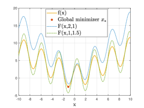
Figure 2: Plot of $f$ (19) and $F$ (18) for two choices of $Y^{1},Y^{2}$. $f$ is continuous, differentiable, nonconvex and admits a unique minimizer at $x_{\star}=-1.119$. The effect of $Y^{1}$ is to stretch the function along the $y$-axis (blue dotted line), while the one of $Y^{2}$ is to amplify the oscillations of $f$ (green dash-dotted line).

In the previous example, we have considered a one-dimensional search space ($d=1$) and a two-dimensional random space ($k=2$). Test 3 (Subsection 5.4) aims at extending our analysis to the scenarios $d,k\gg 1$. We choose an example in which we can easily increase such dimensions, namely

$$F(x,A,b)=||Ax-b||^{2}_{2},\quad\textnormal{with}\;A\in\mathbb{R}^{d\times d},b\in\mathbb{R}^{d}$$ (22)

for some $d\geq 1$ and such that $(A,b)$ has finite second moment, and

$$f(x) =\mathbb{E}[F(x,A,b)]=x^{T}Px-2q^{T}x+r,$$ (23)

with $$\;P=\mathbb{E}[A^{T}A],q=\mathbb{E}[A^{T}b],r=\mathbb{E}[||b||_{2}^{2}].$$

The minimization problem associated to $f$ is known in literature as the linear-least squares problem, see e.g. [33]. $f$ defined in (23) admits a unique minimizer

$$x_{\star}=2(P^{T}+P)^{-1}q,\quad\textnormal{provided that $\textnormal{det}(P)\neq 0$.}$$

In Test $3$ we choose

$$A=\begin{bmatrix}Y^{1}&0\\ Y^{2}&Y^{3}\end{bmatrix},\quad b=\begin{bmatrix}Y^{4}\\ Y^{5}\end{bmatrix},\quad\textnormal{with $Y^{1},\ldots,Y^{5}\sim\mathcal{U}(\mathcal{E})$, $\mathcal{E}=[0,2]$, independent},$$ (24)

so that

$$P=\begin{bmatrix}2&1\\ 1&1\end{bmatrix},\quad q=\begin{bmatrix}2\\ 1\end{bmatrix},\quad r=\frac{8}{3}\quad\textnormal{and}\quad f_{\mathbf{Y}}(\mathbf{y})=\frac{1}{(l(\mathcal{E}))^{5}}\text{1}_{\mathcal{E}^{5}}(\mathbf{y}),\quad\textnormal{for any $\mathbf{y}\in E$}.$$

and $d=2,k=5$. We remark that the choice $A_{12}=0$ guarantees the non-singularity of the matrix $P$. For this test, we use the anisotropic CBO specified by the update rule (17) with parameters

$$T=7,\Delta t=1;\quad\lambda=1,\alpha=40,\sigma=0.5;\quad\mu_{0}=\mathcal{U}([-3,3]^{d}).$$ (25)

The choice of anisotropic random exploration process in this experiment has been shown to be more competitive than the isotropic one for problems with a high dimensional search space, thanks to the independence of the parameter constraints of the dimensionality $d$ [16, 22].

5.2 Test 1: Convergence rates for SAA and CBO

In Section 2 we derived the mean-field equation associated to the CBO algorithm (4) in the regimes $M,N\to\infty$ and proved that the result holds regardless of the order in which we perform the limits. In this subsection, we numerically investigate the rates of convergence of the limits presented in the diagram of Theorem 2.2 for the cost function $F$ defined in (18) (and the corresponding expectation $f$ given by (19)) and for the choices (20) and parameters specified by (21).

We begin with the investigation of the rates as $M\to\infty$ and by keeping $N$ fixed. We remark that choosing a low value for $N$ corresponds to exploring the rate where the solution to the CBO algorithm (4) converges to the one of (5) (arrow connecting the pink boxes, on the right), while selecting a high value of $N$ corresponds to determining the rate where the solution to mean-field equation (7) converges to the one of (6) (arrow connecting the white boxes, on the right). In this paragraph we fix $N=5000$ and consider the mean-field regime.

We use the metric presented in Section $2$ of [14] (root mean square error) and consider

$$\left(\mathbb{E}_{\mathbb{P}}\left[\left(\mathbb{E}_{\tilde{\mathbb{P}}}\left[\bar{x}^{\alpha,M}_{t}-\bar{x}^{\alpha,f}_{t}\right]\right)^{2}\right]\right)^{1/2}$$ (26)

to measure the SAA error with respect to $M$. Denote by $(\tilde{\Omega},\tilde{\mathcal{A}},\tilde{\mathbb{P}})$ the probability space on which the random variables $\{X^{i}_{0}\}_{i=1,\ldots,N}$ are defined. We added a further expectation in $\tilde{\mathbb{P}}$ with respect to [14] to accommodate for the stochasticity of the Euler-Maruyama scheme of the CBO algorithm. From a numerical perspective, indicating by $n_{\textnormal{samplesY}}$ the number of times we sample from $\mathbf{Y}$, (26) may use the estimator

$$\left(\frac{1}{n_{\textnormal{samplesY}}}\sum_{l=1}^{n_{\textnormal{samplesY}}}\left(\frac{1}{n_{\textnormal{samplesCBO}}}\sum_{u=1}^{n_{\textnormal{samplesCBO}}}\left[\bar{x}^{\alpha,M,(l),(u)}_{t}-\bar{x}^{\alpha,f,(u)}_{t}\right]\right)^{2}\right)^{1/2}.$$

The three parameters are $M$, $n_{\textnormal{samplesY}}=200$ and $n_{\textnormal{samplesCBO}}=10$.

We present our numerical results in Figure 3. In the first row we proceed as in [12] and investigate the evolution of error (26) as a function of time for three values of $M$. The second row depicts the same error as a function of $M$ and for a fixed $t=T$. Plot (a) shows a decay in the average (26) for increasing $M$ and for each time $t$. This suggests a rate in $M$, which is quantitatively assessed in plot (c). We remark that the choice of the final time in such plot is fixed by the equidistance of the averages during the computation observed in plot (a). The rate $O(M^{-1/2})$ is coherent with the results of the classical theory of SAA, where such rate has been proven for the optimal points estimators provided that $F$ satisfies suitable differentiability and lipschitzianity assumptions around the minimizer [43, 44]. In addition, the fact that the averages (orange, green and purple continuous lines) are non-increasing nor non-decreasing suggest that the error introduced by approximating $\hat{f}_{M}$ with $f$ (and hence $x^{\alpha,M}_{t}$ with $x^{\alpha,f}_{t}$) doesn’t increase during the evolution of the particles’ positions. This observation is again coherent with the classical Monte Carlo theory, see [14, 44, 41].

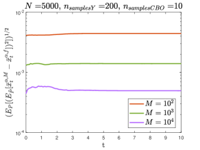
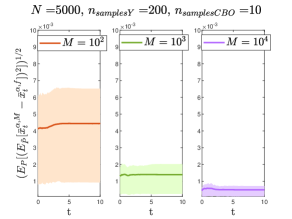
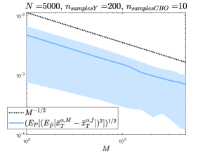
Figure 3: In the first row, evolution of the average error (26) (denoted by a continuous line) as a function of time for $N=5000$ and $M=10^{2},10^{3},10^{4}$. In the second row, evolution of the same error as a function of $M$ (varying from $10^{2}$ to $10^{4}$ with step $500$) and for $N=5000$ and time $t=T$. The shaded area of plots (b) and (c) indicates the $[0.15,0.85]$ quantile interval related to the uncertainty of repeatedly sampling of $\mathbf{Y}$. Plot (a) has a log-scale on $y$-axis, (b) a natural scale on $y$-axis and (c) a log scale on both axis. The objectives considered are (18) and (19) with (20), parameters are set to (21).

Remark 5.2.

A possible disadvantage of Monte-Carlo (MC)/SAA type techniques is the slow rate of convergence $O(M^{-1/2})$. The exponent $1/2$ is intrinsically related to the choice of the root mean squared error and the MC approach and hence it can’t be improved: however, the overall rate depends also on the variance of the function to be integrated. Several techniques have been proposed in literature to reduce such variance and hence to accellerate the converge rate (see e.g. [14, 44]).

Remark 5.3.

We remark that the rate $O(M^{-1/2})$ of the above diagrams is not attained for any objective function $F$. Indeed, as explained in [43, 44], there is no hope of proving the rate analytically if $F$ is non-differentiable at the minimizer. In the following we provide a numerical example that confirms such observation also in a scenario for the consensus points. The Ackley function in dimension $d=1$ and with zero shifts $B=C=0$ is

$$f(x)=f_{A}(x)=-20\exp(-0.2|x|)-\exp(\cos(2\pi x))+20+e,\quad\textnormal{for $x\in\mathbb{R}^{d}$}.$$

We define

$$F_{A}(x,Y^{1},Y^{2})=F(x,Y^{1},Y^{2})=-20Y^{1}\exp(-0.2|x|)-Y^{2}\exp(\cos(2\pi x))+20+e,\quad\textnormal{for $x\in\mathbb{R}^{d}$}.$$

with $Y^{1},Y^{2}\sim\mathcal{U}([0.1,1.9])$. The effect of $a,b>0$ is to stretch the original Ackley function along the $y$-axis. As $\mathbb{E}[a]=\mathbb{E}[b]=1$, it follows that $\mathbb{E}[F_{A}(x,a,b)]=f_{A}(x)$. If we now choose the same parameters as in Figure 3 and $f=f_{A},F=F_{A}$, we obtain Figure 4, for which the rate $O(M^{-1/2})$ is not observed.

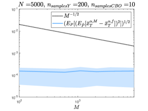
Figure 4: Evolution of the average error (26) as a function of $M$ for $f_{A}$ and $F_{A}$ defined in Remark 5.3. For a detailed description of the parameters used see Figure 3.

Next, we fix $M$ and let $N\to\infty$, as we are interested in the rate of convergence of the interacting particles systems (4) and (5) to the solutions to the mean-field equations (7) and (6) respectively (arrow connecting the pink and white boxes, first and second row resp.). This rate, known as mean-field approximation rate, has been theoretically investigated in the last decade: we mention [23, 24] and [27], where the estimates are extended to stronger metrics than convergence in probability, in particular to $p-$Wasserstein distances (for an introduction on $p-$Wasserstein distances, see e.g. [3, 19]). We consider

$$\mathbb{E}_{\mathbb{P}}\left[\mathbb{E}_{\tilde{\mathbb{P}}}[W_{p}(\mu^{N,M}_{t},\bar{\mu}^{M}_{t})]\right]$$ (27)

$$\approx\frac{1}{n_{\textnormal{samplesY}}}\sum_{l=1}^{\textnormal{samplesY}} \left(\frac{1}{n_{\textnormal{samplesCBO}}}\sum_{u=1}^{n_{\textnormal{samplesCBO}}}W_{p}(\mu^{N,M,(l),(u)}_{t},\bar{\mu}^{M,(l),(u)}_{t})\right),$$

for $p=1,2$, where we have added the expectation on $\mathbb{P}$ with respect to [27] to accommodate for the fact that the cost function $\hat{f}_{M}$ depends on the random sample $\mathbf{Y}$. Here, $\mu^{N,M}_{t},\bar{\mu}^{M}_{t}$ denote the empirical measures associated to the samples $(X^{1}_{t},\ldots,X^{N}_{t})$, for a fixed $N$, and $(X^{1}_{t},\ldots,X^{N_{\textnormal{ref}}}_{t})$, for $N_{\textnormal{ref}}=10^{5}$, solutions to (4). The just-mentioned samples depend on the realization of $\mathbf{Y}$ and on the run of the CBO. From an implementation point of view, we have three parameters: $n_{\textnormal{samplesY}}=200$, $n_{\textnormal{samplesCBO}}=10$ and $N$.

We present our main results in Figure 5, for $M=100$ and $p=1$ in the first row, $p=2$ in the second. The column on the left corresponds to error (27) plotted as a function of time and for three values of $N$, as done in [12]. The right shows the same error plotted as a function of $N$ and for fixed $t=T$. As in Figure 3 (a)-(b), we observe, for a fixed time $t$ and for increasing $N$, a decrease in the average of $W_{p}(\mu^{N,M}_{t},\bar{\mu}^{M}_{t})$. This shows $\mu^{N,M}_{t}\approx\bar{\mu}^{M}_{t}$ in the $p$-Wasserstein distance: numerically this validates the propagation of chaos assumption on the marginals; in addition, the decrease of the three averages as $t$ increases suggests a decrease in the mean-field error as the particles converge to the global minimizer $x_{\star}$ [12]. The rate exponent $1/2$ in Figure 5 (b)-(d) is coherent with the analytical estimates presented in [23, 24, 27].

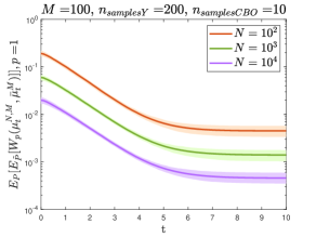
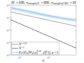
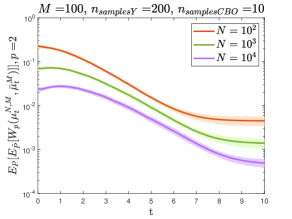
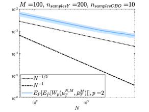
Figure 5: In the column on the left, evolution of the average error (27) (denoted by a continuous line) as a function of time for $M=100$ and $N=10^{2},10^{3},10^{4}$. In the column on the right, evolution of the same error as a function of $N$ (varying from $10^{2}$ to $10^{4}$ with step $500$) and for $M=100$ and time $t=T$. The first row corresponds to the $1$-Wasserstein distance, the second on the $2$-Wasserstein distance. The shaded area indicates the $[0.15,0.85]$ quantile interval related to the uncertainty of repeatedly sampling of $\mathbf{Y}$. Plot (a)-(c) have a log-scale on $y$-axis, while plot (b)-(d) a log scale on both axis. The objectives considered are (18) and (19) with (20), parameters are set to (21).

Remark 5.4.

Changing the value of $M$ in our simulations doesn’t change the qualitative behavior of the plots in Figure 5. Indeed, $M$ governs the quality of the approximation $\hat{f}_{M}\approx f$, but, once it is fixed, $\hat{f}_{M}$ becomes an objective function to which to apply the classical results of the CBO on the mean-field approximation rate [23, 24, 27].

5.3 Test 2: Convergence rates for quadrature and CBO

In Section 3, we derived the mean-field equation on the extended phase space associated to the CBO algorithm (13) in the regime $N\to\infty$ and proved that it coincides with (6) up to a scaling factor. In this subsection we investigate the mean-field type error corresponding to the diagonal in the diagram of Theorem 4.1.

The analysis is similar to the second part of Subsection 5.2. We define the mean-field approximation rate

$$\mathbb{E}_{\tilde{\mathbb{P}}}[W_{p}(\mu^{N}_{t},\bar{\mu}_{t})]\approx\frac{1}{n_{\textnormal{samplesCBO}}}\sum_{u=1}^{n_{\textnormal{samplesCBO}}}W_{p}(\mu^{N,(u)}_{t},\bar{\mu}^{(u)}_{t}),$$ (28)

where $\mu^{N}_{t},\bar{\mu}_{t}$ denote the empirical measures associated to the samples $(X^{1}_{t},\ldots,X^{N}_{t})$, for a fixed $N$, and $(X^{1}_{t},\ldots,X^{N_{\textnormal{ref}}}_{t})$, for $N_{\textnormal{ref}}=10^{5}$, solutions to (13). The error defined in (27) coincides with the error considered in [27].

We present our results in Figure 6 for $p=2$.

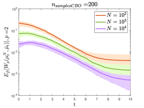
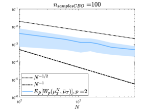
Figure 6: In the column on the left, evolution of the average error (28) for $p=2$ (denoted by a continuous line) as a function of time for $N=10^{2},10^{3},10^{4}$. In the column on the right, evolution of the same error as a function of $N$ (varying from $10^{2}$ to $10^{4}$ with step $500$) and for time $t=T$. The shaded area indicates the $[0.15,0.85]$ quantile interval related to the $n_{\textnormal{samplesCBO}}$ runs of the CBO algorithm. Plot (a) has a log-scale on $y$-axis, plot (b) a log scale on both axis. The objectives considered are (18) and (19) with (20), parameters are set to (21).

The composite midpoint rule has an integration error of order $O(N^{-2/k})$ in the Euclidean distance provided that the integrand is $C^{2}$ in the $y$-component, see e.g. [33]. In our example ($k=2$) this corresponds to

$$|f(x)-\tilde{f}_{N}(x)|\sim O(N^{-1}),\quad\textnormal{for any $x\in\mathbb{R}^{d}$}.$$

In addition, we have that the mean-field approximation rate in the $2$-Wasserstein distance is $O(N^{-1/2})$ [27]. In plot (b) of Figure 6, we deduce that the overall error (28) is $O(N^{-1/2})$, hence it is governed by the rate of the CBO. This remark justifies the choice of the composite midpoint rule rather than high order quadrature formulas.

The computational complexity of the CBO algorithm (13) numerically discretized by update rule (17) is now discussed. For each iterate of the CBO algorithm, calculating $x^{\alpha,N}_{t}$ requires $O(N)$ computations and evaluating the quadrature formula requires $O(N\cdot N^{2})$ evaluations of the objective function $F$. The selection of number of nodes equal to the number of particles in the algorithm is chosen for the convergence analysis. In order to speed up computations, we can use a composite midpoint formula with $N_{0}=\lceil N^{1/2}\rceil$ nodes ($N_{0}$ is so that the rate $(N_{0})^{-1}$ of the midpoint composite rule coincides with the rate $N^{-1/2}$ of the CBO). This leads to $O(N\cdot N_{0}^{2})$ evaluations of $F$ and to Figure 7, which shows similar behavior. Even so, the theoretical analysis does not cover this case.

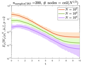
Figure 7: Evolution of the average error (28) obtained by using $N_{0}=\lceil N^{1/2}\rceil$ points in the quadrature formula rather than $N$. For a detailed description of the parameters used see Figure 6.

5.4 Test 3: Convergence rates for quadrature and CBO for $k\geq 2$

In this section we investigate an increase in the dimension of the random space $k$ on the rate of convergence $O(N^{-2/k})$. We evaluate the aforementioned error for the cost function $F$ defined in (22) (and $f$ defined in (23)) for the choices (24) ($k=5$ and $d=2$) and parameters specified by (25).

We plot our result in Figure 8 for $p=2$. We let $N$ vary from $5$ to $10$ and fix $N_{\textnormal{ref}}=10$. These options aim at speeding up the computational time, as the number of evaluations of $F$ in each iteration of the algorithm is equal to $O(N\cdot N^{k})$. We also observe that we may reduce such complexity to $O(N\cdot N(\log N)^{k-1})$ by using sparse grids [13]. For completeness, we also draw error (28) for $F$ defined in (22) for $k=2$ (and $d=1$), which corresponds to the choices

$$A=Y^{1},\quad b=Y^{2},\quad\textnormal{with $Y^{1},Y^{2}\sim\mathcal{U}([0,2])$, independent}.$$ (29)

In the scenarios $k=2$ and $k=5$ the same rate $O(N^{-1/2})$ is observed. This result may be explained by the fact that we have approximated $f$ with $\tilde{f}_{N}$ and we are measuring the convergence rate of the CBO algorithm. This yields the rate $O(N^{-1/2})$. We observe that the scenarios differ in that the error for $k=5$ is larger than the one for $k=2$. This is expected, as for a given $N$, the accuracy of the quadrature formulas in the Euclidean norm are $O(N^{-2/5})$ and $O(N^{-1})$ respectively. Hence, we expect a bigger constant at the decay rate of the former method.

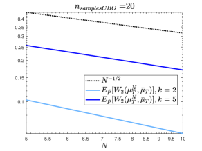
Figure 8: Evolution of the average error (28) as a function of $N$, for $p=2,t=T$. The objectives considered are (22) and (23) for the scenarios $d=2,k=5$ (choice (24), dark blue line) and $d=1,k=2$ (choice (29), light blue line). Parameters of time discretization and CBO are set to (21). The plot has log scales on both axis.

6 Summary and conclusion

We now summarize the main advantages and disadvantages of the two approaches presented in the manuscript, namely of the SAA approach and the quadrature approach. The following analysis is based on our examination of the numerical results and on [1, 43, 44, 41], in which comparisons between Monte-Carlo (MC) type and deterministic approaches are carried out.

The MC method may be applied even if $f_{\mathbf{Y}}$ is unknown or is non-smooth, while the quadrature approach requires these. As regards the computational complexity, we start by observing that in the stochastic approach we have a loop on $n_{\textnormal{samplesY}}$ to accommodate for the stochasticity of the random variable $\mathbf{Y}$, which disappears in presence of the deterministic approach. The cost of each iteration of the CBO algorithm is reported in Table 1.

	SAA approach, algorithm (4)	Quadrature approach, algorithm (13)
Number of evaluations of $F$ to compute $f_{\#}$	$O(N\cdot M)$ to compute $\hat{f}_{M}$	$O(N\cdot N^{k})$ to compute $\tilde{f}_{N}$
Number of evaluations of $f_{\mathbf{Y}}$	$-$	$O(N^{k})$
Computation of $x^{\alpha,\#}_{t}$	$O(N)$ for $\#=M,N$

Table 1: Analysis of the computational complexity for each iteration $t$ of the CBO algorithm for the SAA and quadrature approaches with update rule given by (17). $f_{\#}$ is $\hat{f}_{M}$ or $\tilde{f}_{N}$, see (2), (10) resp.

The quadrature approach is preferred in the scenario of low dimensional random space ($k=1,2$) as a consequence of the absence of the loop on $n_{\textnormal{samplesY}}$ and the comparable number of evaluations of $F$ as described in Table 1. However, as $k$ increases, one may want to opt for the SAA approach where the number of evaluations of $F$ is independent of $k$.

The rate of any deterministic quadrature formula depends on the regularity of the integrand function and on the dimension of the random space $k$ (for instance, in the case of the composite midpoint quadrature rule used in Section 3, the rate is $O(N^{-2/k})$ in the Euclidean norm provided that $F$ $C^{2}$ in the $y$-component). In contrast, the exponent $1/2$ of the MC error is independent of $k$ (robust, but in general slower) and on the smoothness of $F$ in the $y$-component. From the analysis conducted in Subsection 5.2, 5.3 and 5.4, we deduced that the mean-field approximation error (27) and (28) resp. were governed by the $O(N^{-1/2})$-error of the CBO. In particular, even for higher $k$ the overall rate did not deteriorate.

In this work we propose two approaches for solving an optimization problem where the cost function is given in the form of an expectation by means of a stochastic particle dynamics based on consensus. The two methods share the property of replacing the objective function with a suitable approximation, which we chose to be a Monte-Carlo type estimator based on a fixed sample and a quadrature formula, respectively. We conduct a theoretical analysis at the mean-field level and prove that the long time behavior of the first approach is obtained independently of the order in which we perform the limits as the sample size and number of particles tend to infinity. We demonstrate that the identical choice of number of particles and nodes in the second method leads to a mean-field equation in the extended phase space. Numerical experiments are provided to validate the approaches and we investigate their rates of convergence.

We conclude the section by mentioning Quasi-Monte Carlo methods [40, 14], which could be listed as a third approach to solve stochastic programming problem (1). In the literature, quasi MC methods are presented (along with variance-reduction technniques) as an improvement of MC methods that, rather than aiming at reducing the variance of the integrand, accelerate the rate $O(M^{-1/2})$ by substituting the random or pseudo-random sequence with a quasi-random (also known as low discrepancy) sequence. The interest in quasi MC methods relies on the fact that we may recover all the advantages of the quadrature approach, but with the additional freedom of choosing the sequence of discretization points (in the quadrature approach the points $\{\mathbf{y}_{j}\}_{j=1,\ldots,N}$ are fixed and must be chosen according to the quadrature rule).

References

- [1] G. Albi, S. Merino-Aceituno, A. Nota, and M. Zanella. Trails in Kinetic Theory. Springer, 2021.
- [2] G. Albi, L. Pareschi. Binary interaction algorithms for the simulation of flocking and swarming dynamics. Multiscale Modeling & Simulation, 11(1):1–29, 2013.
- [3] L. Ambrosio, N. Gigli, and G. Savaré. Gradient flows: in metric spaces and in the space of probability measures. Springer Science & Business Media, 2005.
- [4] L. Bianchi, M. Birattari, M. Chiarandini, M. Manfrin, M.and Mastrolilli, L. Paquete, O. Rossi-Doria, and T. Schiavinotto. Metaheuristics for the vehicle routing problem with stochastic demands. In Parallel Problem Solving from Nature-PPSN VIII: 8th International Conference, Birmingham, UK, September 18-22, 2004. Proceedings 8, pages 450–460. Springer, 2004.
- [5] L. Bianchi, M. Dorigo, L. M. Gambardella, and W. J. Gutjahr. A survey on metaheuristics for stochastic combinatorial optimization. Natural Computing, 8:239–287, 2009.
- [6] P. Billingsley. Probability and measure. John Wiley & Sons, 2017.
- [7] C. Blum and A. Roli. Metaheuristics in combinatorial optimization: Overview and conceptual comparison. ACM computing surveys (CSUR), 35(3):268–308, 2003.
- [8] F. Bolley, J. A. Canizo, and J. A. Carrillo. Stochastic mean-field limit: non-lipschitz forces and swarming. Mathematical Models and Methods in Applied Sciences, 21(11):2179–2210, 2011.
- [9] G. Borghi, M. Herty, and L. Pareschi. A consensus-based algorithm for multi-objective optimization and its mean-field description. In 2022 IEEE 61st Conference on Decision and Control (CDC), IEEE, pages 4131–4136, 2022.
- [10] G. Borghi, M. Herty, and L. Pareschi. An adaptive consensus based method for multi-objective optimization with uniform Pareto front approximation. Applied Mathematics & Optimization, 88(2):58, 2023.
- [11] G. Borghi, M. Herty, and L. Pareschi. Constrained consensus-based optimization. SIAM Journal on Optimization, 33(1): 211-236, 2023.
- [12] G. Borghi, and L. Pareschi. Kinetic description and convergence analysis of genetic algorithms for global optimization. Preprint arXiv:2310.08562, 2023.
- [13] H.-J. Bungartz, and M. Griebel. Sparse grids. Acta numerica, 13: 147-269, 2004.
- [14] R. E. Caflisch. Monte carlo and quasi-monte carlo methods. Acta numerica, 7:1–49, 1998.
- [15] J. A. Carrillo, Y. P. Choi, C. Totzeck, and O. Tse. An analytical framework for consensus-based global optimization method. Mathematical Models and Methods in Applied Sciences, 28(6):1037–1066, 2018.
- [16] J. A. Carrillo, S. Jin, L. Li, and Y. Zhu. A consensus-based global optimization method for high dimensional machine learning problems. ESAIM: Control, Optimisation and Calculus of Variations, 27:S5, 2021.
- [17] J. A. Carrillo, C. Totzeck, and U. Vaes. Consensus-based optimization and ensemble Kalman inversion for global optimization problems with constraints. Modeling and Simulation for Collective Dynamics, 195-230, 2023.
- [18] C. Cercignani, R. Illner, and M. Pulvirenti. The mathematical theory of dilute gases, volume 106. Springer Science & Business Media, 2013.
- [19] L.P. Chaintron and A. Diez. Propagation of chaos: a review of models, methods and applications. I. Models and methods. Preprint arXiv:2203.00446, 2022.
- [20] C.-H. Chen and L. H. Lee. Stochastic simulation optimization: an optimal computing budget allocation, volume 1. World scientific, 2011.
- [21] A. Dembo and O. Zeitouni. Large deviations techniques and applications, volume 38. Springer Science & Business Media, 2009.
- [22] M. Fornasier, H. Huang, L. Pareschi, and P. Sünnen. Anisotropic diffusion in consensus-based optimization on the sphere. SIAM Journal on Optimization, 32(3):1984-2012, 2022.
- [23] M. Fornasier, T. Klock, and K. Riedl. Consensus-based optimization methods converge globally. Preprint arXiv:2103.15130, 2021.
- [24] M. Fornasier, T. Klock, and K. Riedl. Convergence of anisotropic consensus-based optimization in mean-field law. In International Conference on the Applications of Evolutionary Computation (Part of EvoStar), pages 738–754. Springer, 2022.
- [25] M. Fornasier, L. Pareschi, H. Huang, and P. Sünnen. Consensus-based optimization on the sphere: Convergence to global minimizers and machine learning. Journal of Machine Learning Research, 22(237):1-55, 2021.
- [26] M. Fornasier, L. Sun. A PDE Framework of Consensus-Based Optimization for Objectives with Multiple Global Minimizers. Preprint arXiv:2403.06662, 2024.
- [27] N.J. Gerber, F. Hoffman and U. Vaes. Mean-field limits for Consensus-Based Optimization and Sampling. Preprint arXiv:2312.07373, 2023.
- [28] F. Golse. The mean-field limit for the dynamics of large particle systems. Journées équations aux dérivées partielles, pages 1-47, 2003.
- [29] W. J. Gutjahr. S-aco: An ant-based approach to combinatorial optimization under uncertainty. In International Workshop on Ant Colony Optimization and Swarm Intelligence, pages 238–249. Springer, 2004.
- [30] W. J. Gutjahr, C. Strauss, and E. Wagner. A stochastic branchand-bound approach to activity crashing in project management. INFORMS journal on computing, 12(2):125–135, 2000.
- [31] S.-Y. Ha, S. Jin, and D. Kim. Convergence of a first-order consensus based global optimization algorithm. Mathematical Models and Methods in Applied Sciences, 30(12):2417–2444, 2020.
- [32] S.-Y. Ha, S. Jin, and D. Kim. Convergence and error estimates for time-discrete consensus-based optimization algorithms. Numerische Mathematik, 147:255–282, 2021.
- [33] R. Hamming. Numerical methods for scientists and engineers. Courier Corporation, 2012.
- [34] D. J. Higham. An algorithmic introduction to numerical simulation of stochastic differential equations. SIAM review, 43(3):525–546, 2001.
- [35] H. Huang and J. Qiu. On the mean-field limit for the consensus-based optimization. Mathematical Methods in the Applied Sciences, 45(12):7814–7831, 2022.
- [36] P.-E. Jabin and Z. Wang. Mean field limit for stochastic particle systems. Active Particles, Volume 1: Advances in Theory, Models, and Applications, pages 379–402, 2017.
- [37] M. Jamil and X.S. Yang. A literature survey of benchmark functions for global optimisation problems. International Journal of Mathematical Modelling and Numerical Optimisation, 4(2):150–194, 2013.
- [38] S. Jin, L. Li and J.-G. Liu. Random batch methods (RBM) for interacting particle systems. Journal of Computational Physics, 400:108877, 2020.
- [39] D. Ko, S.Y. Ha, S. Jin, and D. Kim. Convergence analysis of the discrete consensus-based optimization algorithm with random batch interactions and heterogeneous noises. Mathematical Models and Methods in Applied Sciences, 32(06):1071–1107, 2022.
- [40] H. Niederreiter and A. Winterhof. Quasi-monte carlo methods. In Applied Number Theory, pages 185–306. Springer, 1992.
- [41] L. Pareschi and G. Toscani. Interacting Multiagent Systems: Kinetic Equations and Monte Carlo Methods, volume 32. Springer, 2019.
- [42] R. Pinnau, C. Totzeck, O. Tse, and S. Martin. A consensus-based model for global optimization and its mean-field limit. Mathematical Models and Methods in Applied Sciences, 27(01):183–204, 2017.
- [43] A. Shapiro. Monte carlo sampling methods. Handbooks in operations research and management science, 10:353–425, 2003.
- [44] A. Shapiro, D. Dentcheva, and A. Ruszczynski. Lectures on stochastic programming: modeling and theory. SIAM, 2021.