Know Yourself Better: Diverse Discriminative Feature Learning Improves Open Set Recognition

Abstract

Open set recognition (OSR) is a critical aspect of machine learning, addressing the challenge of detecting novel classes during inference. Within the realm of deep learning, neural classifiers trained on a closed set of data typically struggle to identify novel classes, leading to erroneous predictions. To address this issue, various heuristic methods have been proposed, allowing models to express uncertainty by stating ”I don’t know.” However, a gap in the literature remains, as there has been limited exploration of the underlying mechanisms of these methods. In this paper, we conduct an analysis of open set recognition methods, focusing on the aspect of feature diversity. Our research reveals a significant correlation between learning diverse discriminative features and enhancing OSR performance. Building on this insight, we propose a novel OSR approach that leverages the advantages of feature diversity. The efficacy of our method is substantiated through rigorous evaluation on a standard OSR testbench, demonstrating a substantial improvement over state-of-the-art methods.

1 Introduction

Deep neural networks have exhibited remarkable prowess in classification tasks, spanning domains such as video classification  [20], sentiment analysis  [54], and fault diagnosis  [28]. Nevertheless, practical applications often entail challenges wherein the set of semantic categories during testing may be difficult to exhaust or may dynamically evolve over time, diverging from the training data. Such unforeseen semantic categories, termed open sets, can lead to misclassifications during inference, posing potential catastrophic consequences, as the models lack the ability to express uncertainty with an ”I don’t know” response. Consequently, the imperative for open set recognition (OSR), denoting the capability to discern whether a test sample belongs to a known semantic class within predefined sets, is crucial in real-world scenarios and remains an intricate problem  [51, 14, 35, 16, 13, 49]. In this work, we seek to illuminate OSR through the lens of feature diversity, a perspective hitherto unexplored in existing research. Throughout this text, we designate open set samples as outliers, and the known training classes as inliers.

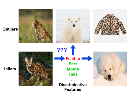
Figure 1: Illustrating the intrinsic link between feature diversity and OSR performance, consider the following scenario: Inliers, i.e., cats and dogs in this example, can be accurately classified by leveraging a discriminative feature like feathers. However, when faced with outliers such as leopards, polar bears, and leopard-patterned jackets, relying solely on the feather feature becomes challenging, especially when these outliers exhibit high similarity in this particular feature. To bolster the model’s ability to robustly identify outliers, additional features, such as ears and tails, need to be learned. This broader set of features enables the model to discern and handle a wider range of outliers effectively.

Creating an exhaustive training dataset that encompasses all potential classes proves unfeasible, given the inexhaustible and sometimes inaccessible nature of open sets in real-world scenarios. Consequently, certain OSR approaches resort to the synthesis of outliers through generative models  [51, 14, 35]. In these methodologies, synthetic outliers are strategically generated to be perplexing samples, exhibiting a high degree of similarity to the inliers. The training of the classifiers involves a combination of these synthetic outliers and genuine inliers. This technique of synthesizing confusion samples echoes the principles of adversarial training, wherein the adjustment of instance discrimination difficulty influences the features the model learns  [42, 18, 7]. The synthetic samples, designed to be semantically akin to the inliers, contribute to a broader feature set that the model must acquire. Therefore, training models with both inliers and synthetic confusing outliers necessitates the learning of a more comprehensive set of features.

In addition to outlier synthesis, several OSR methods aim to refine the learning objectives of discriminative classifiers to enhance their resilience to outliers  [16, 13, 49, 39, 31, 8]. The foundational premise of these approaches is rooted in the notion that instances from the same classes should exhibit proximity, while those from different classes should be distanced  [16, 49, 31]. This fundamental principle, akin to the widely employed metric in traditional feature selection, filters out task-irrelevant features [30]. The metric’s efficacy is heightened when features lack correlation, resulting in a larger metric value (theoretical proof is in Appendix A.1). Consequently, this principle guides the models toward learning more label-relevant features.

In a recent study  [46] it was observed that commonly employed training strategies for supervised classification, such as data augmentation, label smoothing  [33], and extended training epochs, can improve OSR. However, the specific reasons behind these improvements were not explicitly provided. Data augmentation can not only generate more samples and encourage the models to learn invariant features but also facilitates the capture of informative yet challenging-to-learn features  [45]. These features are often susceptible to neglect due to their relatively minor contributions to loss reduction during training. Data augmentation can elevate their significance during training. The models can hence acquire more diverse features.

It has been observed in  [44] that the supervised neural classifiers trained with label smoothing can achieve higher accuracy and label smoothing can contribute to creating tighter and more separated class clusters in latent space, which is aligned with the learning objectives outlined above. Furthermore, for most loss functions applied for deep supervised classifiers, such as cross-entropy and metric learning  [21], since the inter-class shared features cannot contribute to decreasing the loss functions, the models ignore the mutual features among classes. The ignored features can however essential for characterizing multiple inlier classes and discriminating outliers. For example, if the inliers are balls with distinct patterns, the mutual features between the balls, such as shape, can be ignored and it can degrade OSR performances if the outliers exhibit similar patterns. The sustained reduction of the loss function over epochs implies a greater likelihood of models assimilating a more extensive set of features. Both cross-entropy and metric learning are inherently driven by the objective of maximizing the mutual information between the features and corresponding labels  [4]. Acquiring additional discriminative features can amplify the mutual information (theoretical proof is in Appendix A.2).

Building upon the aforementioned analyses and insights, we posit our hypothesis that increasing feature diversity can improve OSR. Feature diversity refers to the variety and richness of discriminative features that a model can learn from the data. It can be intuitively understood in the way that with the increasing of feature diversity, the models have more comprehensive knowledge to model each inlier class. This expanded knowledge base allows for nuanced comparisons between inliers and outliers, increasing the likelihood of accurate OSR. (An intuitive example is in Figure 1).

To empirically substantiate our hypothesis, we conduct preliminary experiments in Section 3. We employ ensembles of features extracted from supervised contrastive learning (SupCon) models, each trained with different temperatures. As outlined in 3.1 the SupCon models with different temperatures emphasize different subsets of the features and the ensemble through concatenating the features can hence naively increase feature diversity. The experimental results unequivocally support our hypothesis. This underscores the pivotal role of feature diversity in augmenting the model’s capability to discern outliers effectively.

Expanding upon our preliminary results and considering efficiency, we propose to enable one single SupCon model to acquire diverse features as the ensembles by applying a temperature modulation method. The evaluation results show that the proposed method can outperform the state-of-the-art OSR approaches on standard testbenches. Our contributions can be summarized as below:

• We identify and substantiate the correlation between the label-relevant feature diversity and OSR performances.

• We propose a method to let supCon models learn more diverse features and obtain state-of-the-art results.

Notations Throughout this paper, we use uppercase letters, e.g., $\mathbf{X}$, $\mathbf{Y}$, and $\mathbf{Z}$ to represent sets, and lowercase letters, such as $\mathbf{x}$, $\mathbf{y}$, and $\mathbf{z}$, to represent samples of sets. Specifically, $\mathbf{X}$, $\mathbf{Y}$, and $\mathbf{Z}$ refer to sets of data, labels, and features respectively. Furthermore, the vectors are denoted using bold letters, whereas scalars are represented using plain letters, e.g., for a vector $\mathbf{z}$, $z_{i}$ refers to one of its elements.

2 Related work

In this section, we cover the most pertinent works and a concise history of open set recognition. For an in-depth exploration of the OSR methods used later as baselines in Section 5, see Appendix D.

Open Set Recognition (OSR) concerned with identifying samples from novel classes during inference. Scheirer et. al pioneered the formalization of OSR, employing support vector machines to project inliers into a slab-shaped space defined by two hyperplanes. The samples outside the hyperplanes are deemed outliers  [43].

In recent years, there has been a surge in the development of OSR methods tailored for deep neural networks. Bendale et. al have revealed that the activation patterns in the penultimate layers of deep classifiers can exhibit distinct characteristics for inliers and outliers  [3]. Subsequently, OSR methods for discriminative models can be broadly categorized into two main groups, namely synthesizing outliers  [51, 14, 35] and designing training objectives that enhance intra-class tightness and inter-class separation in the representation space [16, 13, 49, 39, 31, 8]. Both categories are introduced in Section 1.

Besides relying solely on discriminative classifiers, a bunch of works apply extra models, e.g., generative models, to learn representations of inliers [38, 50, 53, 6]. In [38], a class-conditioned auto-encoder is trained on inliers, and their reconstruction errors are modeled using extreme value distributions to identify outliers during inference. Similarly, [53] employs a flow-based model to characterize the distribution of inliers. The estimated likelihood of testing samples given by the flow-based model is then utilized for detecting outliers through thresholding. Although these approaches are aimed at increasing feature richness, which is similar to our hypothesis, they didn’t notice the label relevance of the features. Models can learn low-level or instance-specific features, which are not desired.

3 Preliminaries

3.1 Background: Supervised Contrastive Learning

3.1.1 Overview

Supervised contrastive learning (SupCon) [23] originates from multi-view self-supervised contrastive learning [10] and InfoNCE [37] that intended to preserve the mutual information between the time series data at current timestamp and their contexts. In contrastive learning, the learning objective aims to enclose the anchors with their positive peers and repel the negative samples in feature space. For self-supervised contrastive learning, the positive samples are normally the original samples and their augmented versions. Therefore, self-supervised contrastive learning relies greatly on data augmentation for feature learning [40].

In SupCon, the positive pairs consist of the original and augmented versions of the anchors as well as the other samples from the same classes, and the negative pairs are those from different classes. Its loss function, $L_{SupCon}$, is demonstrated in Equation (1). For the representation of an anchor sample, $\textbf{z}_{i}$, that indexed by $i$, $P(i)$ stands for the index set of all its positive pairs, $\textbf{z}_{p}$, whereas $N(i)$ is the index set of negative pairs. And $A(i)$ refers to the index set of all the samples, i.e., $A(i)=P(i)\bigcup N(i)$. Temperature $\tau$ is a hyperparameter that scales the cosine similarities between the positive and negative pairs and lays effects on the feature learning processes, which will be studied in detail later. In the following text, we use $s_{ip}$ and $s_{in}$ to denote the cosine similarities between the positive and negative pairs respectively, i.e., $s_{ip}=\textbf{z}_{i}\cdot\textbf{z}_{p}$, and $s_{in}=\textbf{z}_{i}\cdot\textbf{z}_{n}$. An intuitive understanding on Equation (1) is it aims to learn features that can maximize the similarities between the positive pairs and minimize the similarities between the negative pairs.

$$\begin{split}&\mathcal{L}_{SupCon}=\sum_{i\in I}\frac{-1}{|P(i)|}\sum\limits_{p\in P(i)}\log\frac{\exp\left(\textbf{z}_{i}\cdot\textbf{z}_{p}/\tau\right)}{\sum\limits_{a\in A(i)}\exp\left(\textbf{z}_{i}\cdot\textbf{z}_{a}/\tau\right)}\\ &=\sum_{i\in I}\frac{-1}{|P(i)|}\sum\limits_{p\in P(i)}\log\frac{\exp\left(\frac{s_{ip}}{\tau}\right)}{\sum\limits_{p\in P(i)}\exp(\frac{s_{ip}}{\tau})+\sum\limits_{n\in N(i)}\exp(\frac{s_{in}}{\tau})}\\ &\propto\sum_{i\in I}\sum\limits_{p\in P(i)}\left[-\frac{s_{ip}}{\tau}+\log\left(\sum\limits_{p\in P(i)}\exp(\frac{s_{ip}}{\tau})+\sum\limits_{n\in N(i)}\exp(\frac{s_{in}}{\tau})\right)\right]\end{split}$$ (1)

SupCon has been shown to be superior to cross-entropy loss in inlier classification, robustness to image corruptions, and transfer learning since it can learn more generalizable features [23]. SupCon has often been applied to multiple similar tasks of OSR, such as out-of-domain detection [52], and anomaly detection [22].

Moreover, contrastive learning has been repeatedly studied from the perspective of, for example, feature learning [42, 41] and training dynamics [32]. The preliminary and the main methods in this work rely on manipulating the hyperparameter temperature ($\tau$), which plays a crucial role in deciding which type of features the model learns. It will be introduced in the following text.

3.1.2 Temperature and Feature Learning

The temperature $\tau$ in contrastive learning has been explored in multiple previous works [42, 26, 47]. However, these works are intended for self-supervised learning settings. We study the effects given by $\tau$ in supervised contrastive learning in this work.

We analyze the gradients of $\mathcal{L}_{SupCon}$ with respect to $s_{ip}$ and $s_{in}$ between each positive and negative pair respectively (see Equation (2) and (3)) to understand how $\tau$ affects the learning process. The detailed gradient derivation processes of Equation (2) and (3) are in Appendix C.2.

For each positive pair, $\mathbf{z}_{i}$ and $\mathbf{z}_{p}$, $s_{ip}$ is supposed to increase when $\mathcal{L}_{SupCon}$ decreases. We simulate the change of $\frac{\partial\mathcal{L}_{SupCon}}{\partial s_{ip}}$ under different $\tau$ settings to explore how the value of $\tau$ affects the change of $\frac{\partial\mathcal{L}_{SupCon}}{\partial s_{ip}}$ and $s_{ip}$ when the positive samples show variant similarities to the anchors. We plot the value of $\frac{\partial\mathcal{L}_{SupCon}}{\partial s_{ip}}$ versus $s_{ip}$ under different $\tau$ settings to visualize the effects (see the left subplot in Figure 2). It can be found that the gradient values are always small for larger $\tau$s no matter how $s_{ip}$ changes. With the decrease of $\tau$, the gradients increase greatly (we focus on the absolute values here since $s_{ip}$ increases during training), especially for smaller $s_{ip}$. We can then conclude that small $\tau$s are more effective for increasing the intra-class similarities, especially when $s_{ip}$ is small.

$$\begin{split}\frac{\partial\mathcal{L}_{SupCon}}{\partial s_{ip}}&\propto-\frac{1}{\tau}+\frac{\frac{1}{\tau}\exp(\frac{s_{ip}}{\tau})}{\sum\limits_{p\in P(i)}\exp(\frac{s_{ip}}{\tau})+\sum\limits_{n\in N(i)}\exp(\frac{s_{in}}{\tau})}\\ &=\frac{1}{\tau}\left[softmax(\frac{s_{ip}}{\tau})-1\right]\end{split}$$ (2)

Similarly, we plot the values of $\frac{\partial\mathcal{L}_{SupCon}}{\partial s_{in}}$ with respect to $s_{in}$ with different $\tau$ settings in the right subplot of Figure 2. The gradients almost vanish when $\tau$ is small. Hence, larger $\tau$s are more beneficial for decreasing the inter-class dissimilarities. It has been found in previous works as well that the negative samples closest to the anchors receive the highest gradient in self-supervised contrastive learning [26, 47], which aligns with our findings here.

$$\begin{split}\frac{\partial\mathcal{L}_{SupCon}}{\partial s_{in}}&\propto\frac{\frac{1}{\tau}\exp(\frac{s_{in}}{\tau})}{\sum\limits_{p\in P(i)}\exp(\frac{s_{ip}}{\tau})+\sum\limits_{n\in N(i)}\exp(\frac{s_{in}}{\tau})}\\ &=\frac{1}{\tau}softmax(\frac{s_{in}}{\tau})\end{split}$$ (3)

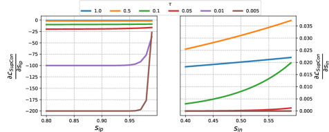
Figure 2: Left: Plots of $\frac{\partial\mathcal{L}_{SupCon}}{\partial s_{ip}}$ values with respect to $s_{ip}$ under different $\tau$ settings. Right: Plots of $\frac{\partial\mathcal{L}_{SupCon}}{\partial s_{in}}$ values with respect to $s_{in}$ under different $\tau$ settings (the curves of $\tau=0.01$ and $\tau=0.005$ are overlapped).

Based on the above analysis that is similar to SupCon. Large $\tau$ is more beneficial for distancing the classes whereas small $\tau$ can make the intra-class samples more compact. Furthermore, as shown in Figure 2 low temperatures can greatly increase $\frac{\partial\mathcal{L}_{SupCon}}{\partial s_{ip}}$, especially for low $s_{ip}$ positive samples, the models can thus learn more class-discriminative features that are hard to be learned with large $\tau$. We name these features using hard features in the following text whereas the rest are referred as easy features.

Both the hard and easy features are essential for open set recognition. As pointed out in Section 1 and Appendix A.1 that more features for discriminating the inlier classes can improve OSR. We will demonstrate in the next subsection that the ensemble of features learned using different temperatures can improve both OSR and inlier classification.

3.2 Preliminary Experiments

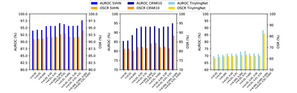
Figure 3: Plots on AUROC and OSCR exhibited by the features (ensembles) from supervised contrastive learning models trained using various temperatures on datasets of (from left to right) SVHN, CIFAR10, and TinyImagenet. Feature ensembles can surpass single models seen from both AUROC and OSCR. The performance exhibits an upward trend with an increase in the number of ensemble members.

To empirically verify our hypothesis in Section 1 asserting a correlation between feature diversity and open set recognition performance, we conduct experiments by creating ensembles of the deep features derived from by SupCon models. As previously mentioned, SupCon models trained with different temperatures exhibit the ability to emphasize or suppress various types of discriminative features in data. Leveraging this characteristic, We ensemble the features extracted from SupCon models trained with variant temperatures to diversify the features employed for recognizing open set samples.

We train SupCon models with $\tau_{0}=0.05,\tau_{1}=0.01,\tau_{2}=0.005$ and concatenate the features extracted by the last layer of the headers (see Figure 5 for an illustration). We use the experiment settings outlined in Section 5.1. Additionally, we follow the framework in Section 4.3 for OSR and classifying inliers using Mahalanobis distances. We record 12 groups of results of different combinations of temperatures, namely $\tau_{0}$, $\tau_{1}$, $\tau_{2}$, $\tau_{0}\&\tau_{0}$, $\tau_{1}\&\tau_{1}$, $\tau_{2}\&\tau_{2}$, $\tau_{0}\&\tau_{1}$, $\tau_{1}\&\tau_{2}$, $\tau_{0}\&\tau_{0}\&\tau_{0}$, $\tau_{1}\&\tau_{1}\&\tau_{1}$, $\tau_{2}\&\tau_{2}\&\tau_{2}$, $\tau_{0}\&\tau_{1}\&\tau_{2}$ for each three datasets, SVHN, CIFAR10, and TinyImagenet. The results are presented in Figure 3.

It can be read from Figure 3 that, for both OSR and close set classification, feature ensembles outperform individual models. Notably, the performance of three ensembles, $\tau_{0}\&\tau_{1}\&\tau_{2}$, can surpass the state-of-the-art OSR approaches (see Table 1 and 2). Considering that even the models trained using the same temperature cannot learn completely the same features. we evaluate the ensemble of features from these models, e.g., $\tau_{1}\&\tau_{1}$, $\tau_{1}\&\tau_{1}\&\tau_{1}$, to eliminate the effects of such occasions. Despite these efforts, the ensembles incorporating features from different temperatures consistently exhibit superior performance. These empirical findings robustly indicate a positive correlation between class-related feature diversity and open set recognition.

Furthermore, for more insights on these results, we provide tSNE visualization of the features and offer detailed discussions in discussion in Appendix C.1. The ensembled features exhibit improved separation among samples from different classes, particularly for those samples that are susceptible to misclassification. This enhanced separation not only suggests superior OSR performances but also indicates improved close set classification performances.

4 Method

Motivated by our hypothesis and its validation in Section 1 and 3, we propose a method in this section that can enable one single SupCon model to learn diverse features through modulating the temperature. This method can largely reduce computational load compared with the ensemble and achieve better performances. We will first analyze why feature suppression happens in SupCon and how the temperature plays its role. Then we will introduce our method as well as the entire framework for open set recognition.

4.1 Feature Forgetting in Contrastive Learning

It has been found in previous work that training contrastive learning models using variant temperatures successively can cause feature forgetting, i.e., the acquiring of new hard features is at the expense of old easy features [41, 42]. We have observed in experiments as well that the decrease of $\tau$ during training can trigger the increase of $s_{in}$. Figure 4 illustrates the change of $s_{ip}$ and $s_{in}$ during training when step-wise evenly changing $\tau$. We think such phenomenon is because the absolute change of $\frac{\partial\mathcal{L}_{SupCon}}{\partial s_{ip}}$ can be much larger than $\frac{\partial\mathcal{L}_{SupCon}}{\partial s_{in}}$ when decreasing $\tau$, i.e., $|\Delta\frac{\partial\mathcal{L}_{SupCon}}{\partial s_{ip}}|\gg|\Delta\frac{\partial\mathcal{L}_{SupCon}}{\partial s_{in}}|$. It can be found from Figure 2 that the numerical distances between the curves in $\frac{\partial\mathcal{L}_{SupCon}}{\partial s_{ip}}\>\mathsf{vs.}\>s_{ip}$ are in different orders of magnitude than these in $\frac{\partial\mathcal{L}_{SupCon}}{\partial s_{in}}\>\mathsf{vs.}\>s_{in}$. Therefore, the models put much more attention on increasing $s_{ip}$ than decreasing $s_{in}$, which can cause the forgetting of the easy features learned before. Furthermore, we have observed during experiments that $s_{in}$ increases instantly after $\tau$ increases, which means the forgetting happens very fast. We will discuss this point further in Appendix E.1. Thus, one idea to reduce the forgetting is to balance the gradients for $s_{in}$ and $s_{ip}$ through a slow and smooth change of the temperatures.

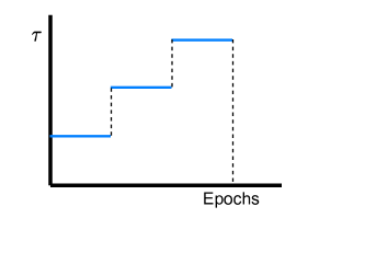
Figure 4: Change of $s_{ip}$ and $s_{in}$ during training on CIFAR10 when evenly step-wise changing $\tau$ from 0.05 to 0.03. $s_{in}$ increases during training. The new model is trained based on the $\tau_{max}$ model.

4.2 Temperature Modulation for SupCon

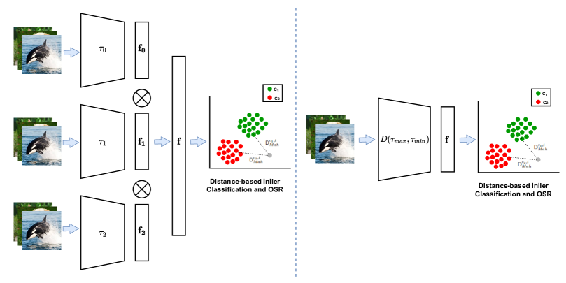
Figure 5: Illustration of our feature concatenation method used in preliminary experiments (left) and smooth SupCon (right). The final classification and outlier scores are all computed using the Mahalanobis distances between the testing sample and each class center.

Based on the analysis above and inspired by [26], we try to modulate the temperatures slowly using different strategies (see 4 in Ablation Study). Among all the tests, modulation with cosine function in Equation (4) can show the best OSR performance. We, therefore, use the cosine function to modulate the temperature. In Equation (4), $\tau_{max}$ and $\tau_{min}$ stand for the upper and lower bound of the temperatures, and $T$ is the cosine period. The new model is trained on top of the $\tau_{max}$ model. We call our method Smooth SupCon.

$$\tau_{t}=(\tau_{max}-\tau_{min})*\frac{1+\cos(2\pi/T*t)}{2}+\tau_{min}$$ (4)

4.3 Overall Framework

Instead of thresholding the logits that outputted by the final classification layers, we rely on Mahalanobis distances, $\mathsf{D}_{Mah}^{c,t}$ in Equation  (5), between the representations of testing samples $\mathbf{z}_{t}$ and inlier samples of class $c$, which are represented using center $\mathbf{\mu}_{c}$ and intra-class covariance $\mathbf{\Sigma}_{c}$ in feature space, to detect outliers. $n_{C}$ stands for the number of training samples in class $c$. Mahalanobis distance has often been applied in anomaly detection [19], out of distribution detection [27], as well as open set recognition [29].

$\mathsf{D}_{Mah}^{c,t}$ is then compared with a pre-defined threshold $\tau_{Mah}$ to detect outliers. $\mathsf{D}_{Mah}^{c,t}$ is utilized for classifying inliers as well. The final classification score is the softmax over $\mathsf{D}_{Mah}^{c,t}$ to each class center.

$$\begin{gathered}\mathsf{D}_{Mah}^{c,t}=(\mathbf{z}_{t}-\mathbf{\mu}_{c})^{T}\mathbf{\Sigma}_{c}^{-1}(\mathbf{z}_{t}-\mathbf{\mu}_{c}),\\ \mathbf{\mu}_{c}=\frac{1}{n_{c}}\sum_{i=0}^{n_{c}-1}\mathbf{z_{i}},\mathbf{\Sigma}_{c}=(\mathbf{Z}_{c}-\mathbf{\mu}_{c})^{T}(\mathbf{Z}_{c}-\mathbf{\mu}_{c})\end{gathered}$$ (5)

5 Experiments

5.1 Settings

Datasets. Following in the OSR testbench in literature [46, 9, 35], we evaluate our methods on six split Protocols, namely MNIST, SVHN, CIFAR10, CIFAR+10, CIFAR+50, and TinyImagenet created using the source datasets of MNIST [12], SVHN [36], CIFAR10 [1], CIFAR100 [2], and TinyImagenet [11]. The number of training classes (denoted using K) and the total number of testing classes (denoted using M) and their data sources of each protocol are shown in Table 5 in Appendix B. The complexity of each protocol is measured using openness, $O=1-\sqrt{K/M}$, i.e., the portion of outlier classes over the total number of classes.

Metrics Since the OSR approaches require setting the thresholds manually, a threshold-independent metric, the area under the receiver operating characteristic (AUROC) curve [34] is one of the most commonly utilized metrics to evaluate the OSR methods since a direct result comparison with different thresholds is not reasonable. In the AUROC curve, the true positive rate is plotted against the false positive rate by varying the threshold. The higher the AUROC is, the better the model can distinguish outliers from the inliers. In our work. we vary the Mahalanobis distances of each testing sample to the closest training class in representation space to create the AUROC curves.

We use Open Set Classification Rate (OSCR) [13] to evaluate the inlier classification performance. In OSCR, the testing samples are split into inlier class samples $D_{c}$ and outlier class samples $D_{u}$. For $D_{c}$, the Correct Classification Rate (CCR) is calculated as in Equation (6), which is the fraction of the samples in $D_{c}$ that are correctly classified as $\hat{c}$ with the probability greater than a threshold $\theta$. For $D_{u}$, the False Positive Rate (FPR) is computed as in Equation (7), which is the fraction of the samples in $D_{u}$ that are classified as any inlier classes with the probability greater than $\theta$. In OSCR plots, FPR is on x-axis and CCR is on y-axis. The curve can be interpreted as when FPR varies from zero to one, how CCR changes with different thresholds. OSCR aggregates inlier classification and OSR in one metric that can describe the overall performances of both. The higher the OSCR is, the better the model can classify the inliers while guaranteeing the OSR performance.

$$CCR(\theta)=\frac{|\{\mathbf{x}|\mathbf{x}\in D_{c}\bigwedge P(\hat{c}|\mathbf{x})\geq\theta\}|}{|D_{c}|}$$ (6)

$$FPR(\theta)=\frac{|\{\mathbf{x}|\mathbf{x}\in D_{u}\bigwedge{max}_{c}P(c|\mathbf{x})\geq\theta\}|}{|D_{u}|}$$ (7)

Implementation details We use ResNet-18 [17] as the backbone for all the models in this work. We didn’t use any pre-training strategies or rely on any large datasets or foundation models. The data augmentation strategies applied for contrastive learning are standard, i.e., random flip, color jitter, and gray scaling. We use Adam optimizer [24] with momentum to train the models, which is also standard in many contrastive learning works. The hyperparameters settings are in Appendix B.3.

5.2 Results

The AUROC and OSCR results are in Table 1 and 2 respectively. Our two approaches can surpass the state-of-the-art on most testing protocols. Feature ensemble works better than smooth SupCon in general, but the gaps are small. Notably, both of our methods perform extraordinarily well on the TinyImagenet dataset with at least $3\%$ of AUROC.

	MNIST	SVHN	CIFAR10	CIFAR+10	CIFAR+50	Tiny-ImageNet
	$22.54\%$	$22.54\%$	$22.54\%$	$46.55\%$	$72.78\%$	$68.37\%$
Cross Entropy	$97.8$	$88.6$	$67.7$	$81.6$	$80.5$	$57.7$
Openmax [3]	$98.1$	$89.4$	$69.5$	$81.7$	$79.6$	$57.6$
G-Openmax [14]	$98.4$	$89.6$	$67.5$	$82.7$	$81.9$	$58.0$
OSRCI [35]	$98.8$	$90.1$	$69.9$	$83.8$	$82.7$	$58.6$
C2AE [38]	$98.9$	$92.2$	$89.5$	$95.5$	$93.7$	$74.8$
APRL [9]	$99.6$	$96.3$	$90.1$	$96.5$	$94.3$	$76.2$
APRL-CS [9]	$\mathbf{99.7}$	$96.7$	$91.0$	$97.1$	$95.1$	$78.2$
MLS [46]	$99.3$	$97.1$	$93.6$	$97.9$	$\mathbf{96.5}$	$83.0$
OpenAUC [48]	$99.4$	$95.0$	$89.2$	$95.2$	$93.6$	$75.9$
Ensemble SupCon ($\tau_{0}$, $\tau_{1}$, $\tau_{2}$)	$\mathbf{99.7}$	$\mathbf{97.71}$	$\mathbf{94.95}$	$\mathbf{98.1}$	$96.11$	$\mathbf{88.34}$
Smooth SupCon	$\mathbf{99.7}$	$96.1$	$94.02\uparrow$	$96.67$	$95.61$	$86.59\uparrow$

Table 1: The area under the ROC curve (AUROC) (in $\%$) for detecting known and unknown samples (Partial results of the baseline methods are from [9] and [46]). Bold numbers indicate the best results, and $\uparrow$ refers to the results that surpass or are equal to the state-of-the-art.

	MNIST	SVHN	CIFAR10	CIFAR+10	CIFAR+50	Tiny-ImageNet
	$22.54\%$	$22.54\%$	$22.54\%$	$46.55\%$	$72.78\%$	$68.37\%$
Cross Entropy	$99.2$	$92.8$	$83.8$	$90.9$	$88.5$	$60.8$
Openmax [3]	$99.2$	$92.9$	$84.0$	$91.1$	$88.3$	$61.0$
G-Openmax [14]	$99.3$	$93.0$	$84.1$	$92.3$	$90.1$	$60.9$
OSRCI [35]	$99.3$	$93.0$	$84.4$	$92.5$	$90.4$	$61.1$
C2AE [38]	$99.4$	$93.5$	$88.1$	$93.4$	$91.2$	$61.3$
APRL [9]	$99.4$	$94.0$	$86.6$	$93.5$	$91.6$	$62.3$
APRL-CS [9]	$99.5$	$94.3$	$87.9$	$87.9$	$92.9$	$65.9$
MLS [46]	$99.5$	$95.3$	$89.1$	$93.6$	$93.6$	$75.1$
OpenAUC [48]	$99.4$	$93.9$	$85.1$	$92.7$	$91.1$	$62.1$
Ensemble SupCon ($\tau_{0}$, $\tau_{1}$, $\tau_{2}$)	$\mathbf{99.6}$	$\mathbf{96.7}$	$\mathbf{90.3}$	$\mathbf{94.1}$	$\mathbf{93.4}$	$\mathbf{82.3}$
Smooth SupCon	$99.5\uparrow$	$94.54$	$89.67\uparrow$	$89.82$	$89.1$	$81.96\uparrow$

Table 2: The open set classification rate (OSCR) results (in $\%$) on standard testing protocols with openness (Results of the baseline methods are from [9] and [46]). Bold numbers indicate the best results, and $\uparrow$ refers to the results that surpass or are equal to the state-of-the-art.

5.3 Ablation Study

Modulation Strategy	AUROC	OSCR
Fixed	$88.8$	$85.6$
Step	$89.2$	$83.4$
Exponential	$88.1$	$86.2$
Linear	$88.7$	$85.5$
Cosine	$\mathbf{92.8}$	$\mathbf{87.9}$

Table 3: Comparison of OSR and inlier classification performances of the models trained using different temperature modulation strategies. The models are trained and tested under CIFAR10 protocol with the temperature varying from $0.05$ to $0.03$.

	0.05
Fixed	$88.8/83.6$
0.04	$91.8/89.1$
0.03	$92.8/89.9$
0.02	$89.6/88.3$
0.01	$89.9/88.3$

(a)

	0.1
Fixed	$86.1/79.6$
0.09	$88.7/84.7$
0.08	$89.5/87.3$
0.07	$89.6/87.6$
0.06	$86.5/84.8$

(b)

Table 4: Change of AUROC and OSCR (AUROC/OSCR) with different $\tau_{max}$ and $\tau_{min}$ combinations. All the models are trained with 400 epochs and the cosine period of 200 epochs.

Temperature Modulation Strategy We have tested the temperature modulation strategies of step modulation (Step), modulation using the linear function(Linear), modulation using the exponential function (Exponential), and modulation using the cosine function (Cosine). A detailed introduction on these strategies except Cosine is in Appendix B.4.1. All the models are trained with the same temperature changing range (0.05 to 0.03).

The results in Table 4 exhibit that modulation using the cosine function can obtain the best performance. We think the reason lies in the changing trend of the cosine function, which is slow at the beginning and end of each period. According to our observation during experiments using linear modulation, $s_{in}$ increases fastest during these two regimes.

W/O Modulation and the Selection of $\tau_{min}$ We compare the AUROC and OSCR of the models trained w/o changing temperature as well as these with distinct $\tau_{min}$ in Table 4. Unsurprisingly, models with dynamically changing $\tau$ values outperform those trained using fixed single temperatures, which can validate the advantage of our method.

Furthermore, based on our two sets of experiments, we observe a discernible trend where performance undergoes a slight increase before experiencing a subsequent decline. We attribute this behavior to the fact that a very small changing range becomes indistinguishable from a fixed temperature, while a large range may lead to more forgetting of features learned at higher temperatures. The optimal balance between adaptability and feature retention appears to manifest within a moderate changing range.

5.4 Discussion

Drawing insights from the conducted experiments, several conclusions emerge: 1) Temperature modulation proves advantageous for open set recognition, which is the goal of our method; 2) Feature ensemble outperforms feature modulation; 3) Both methods exhibit exceptional performance on the TinyImagenet dataset.

It is no surprise to see 2) that models may experience some degree of feature forgetting even with meticulous modulation. In contrast, ensembles provide a workaround for this issue, enabling the application of a more extensive range of temperatures to effectively learn a more diverse set of features. We think the reason for 3) is the nature of contrastive learning. There are more negative samples for each anchor when training on TinyImagenet, it is then easier for the models to learn more features.

6 Conclusion

In this study, we have delved into the challenge of open set recognition, demonstrating a positive correlation between OSR performance and the diversity of discriminative features learned from inlier data. Capitalizing on this insight, we proposed a novel approach utilizing supervised contrastive learning in conjunction with smoothly changing temperatures, resulting in state-of-the-art performance. We anticipate that our contributions will serve as a catalyst for future research endeavors, inspiring the exploration of diverse feature learning to enhance open set sample detection.

The open world, inherently inexhaustible, eludes direct modeling using existing data, even when extensive. To effectively address open set recognition, our approach focuses on comprehensively modeling its complementary counterpart—the inliers. Learning diverse discriminative features not only proves crucial for OSR but also holds significance for broader model generalization, safeguarding against shortcut learning [15] and enhancing domain generalization [li2021simple]. Furthermore, besides tuning the learning objectives, there exists ample opportunity to explore methods for manipulating the data, aiming at further enriching the diversity of features learned by the models. In future work, we will explore effective data augmentation approaches in this direction.

Supplementary Material

Appendix A Theoretical Proof

Theorem A.1.

The more class-relevant features that the models have learned, the more robust it is to the outliers.

As discussed in Section 1, many learning objectives of OSR methods for discriminative models are to distance the features of distinct inlier classes. Assume that a discriminative model is trained by two inlier classes $A$ and $B$. The feature vector $Z$ consists of $N$ independent elements, i.e., $Z=[z_{0},z_{1},...,z_{N-1}]$. We use the metric proposed in [5] in Equation (8) based on KL divergence to measure the feature separability:

$$\text{DIV}_{\textsubscript{A,B}}=\sum_{i}P(z_{i}|c=A)\log{\frac{P(z_{i}|c=A)}{P(z_{i}|c=B)}}$$ (8)

Equation (8) is the KL divergence between $P(z_{i}|c=A)$ and $P(z_{i}|c=B)$, i.e., $D_{KL}(P(z_{i}|c=A),P(z_{i}|c=B))$. Since $z_{0},z_{1},...,z_{N-1}$ are independent from each other, then $\max\text{DIV}_{\textsubscript{A,B}}=\sum_{i}\max D_{KL}(P(z_{i}|c=A),P(z_{i}|c=B))$. We use $D_{KL}^{i}$ to denote $D_{KL}(P(z_{i}|c=A),P(z_{i}|c=B))$, i.e., $D_{KL}^{i}=D_{KL}(P(z_{i}|c=A),P(z_{i}|c=B))$.

Assume that, for each feature element $z_{i}$, it can either be a discriminative feature for class $A$ or $B$ or a non-discriminative feature, such as noises. If $z_{i}$ is a discriminative feature for class $A$ or $B$, then $D_{KL}^{i}\gg 0$. We use Gaussian distributions to model $P(z_{i}|c=A)$ if it is discriminative feature for class $A$, i.e., $P(z_{i}|c=A)\sim\mathcal{G}(f_{A_{i}},\sigma_{d_{1}}^{2})$, $P(z_{i}|c=B)\sim\mathcal{G}(f_{B_{i}},\sigma_{d_{2}}^{2})$, in which $|f_{A_{i}}-f_{B_{i}}|\gg 0$, $|f_{B_{i}}|\approx 0$, and $\sigma_{d_{1}}^{2}\ll 1$, $\sigma_{d_{2}}^{2}\ll 1$. $f_{A_{i}}$ and $f_{B_{i}}$ are the mean values of $z_{i}$. It is a similar case if $z_{i}$ is a discriminative feature for class $B$. For the sake of simplicity, we use $\sigma_{d_{1}}^{2}$ and $\sigma_{d_{2}}^{2}$ to represent the covariances of the distributions of all discriminative features in their belonged and non-belonged classes respectively, since the covariances are all extremely small values. Furthermore, we use Gaussian distributions as well to model $P(z_{i}|c=A)$ and $P(z_{i}|c=B)$ if it is not a discriminative feature, i.e., $p(z^{i}|c=A)\sim G(f_{A_{i}},\sigma_{n_{1}}^{2})$ and $p(z^{i}|c=B)\sim G(f_{B_{i}},\sigma_{n_{2}}^{2})$, in which $\sigma_{n_{1}}^{2}\gg 1$ and $\sigma_{n_{2}}^{2}\gg 1$. Similarly, we use $\sigma_{n_{1}}^{2}$ and $\sigma_{n_{2}}^{2}$ to represent the covariances in the distributions of all non-discriminative features of the samples in class $A$ and $B$ since $\sigma_{n_{1}}^{2}$ and $\sigma_{n_{2}}^{2}$ are extremely large.

The KL divergence between two Gaussian distributions, $p\sim\mathcal{N}(\mu_{1},\sigma_{1}^{2})$ and $q\sim\mathcal{N}(\mu_{2},\sigma_{2}^{2})$, is as in Equation (9):

$$D_{KL}(p,q)=\log\frac{\sigma_{2}}{\sigma_{1}}+\frac{\sigma_{1}^{2}+(\mu_{1}-\mu_{2})^{2}}{2\sigma_{2}^{2}}-\frac{1}{2}$$ (9)

If $z_{i}$ is discriminative feature for $A$ or $B$:

$$\begin{split}D_{KL}^{i}&=\log\frac{\sigma_{d_{2}}}{\sigma_{d_{1}}}+\frac{\sigma_{d_{1}}^{2}+(f_{A_{i}}-f_{B_{i}})^{2}}{{2\sigma_{d_{2}}^{2}}}-\frac{1}{2}\\ &\approx\log 1+\frac{1}{2}+\frac{(f_{A_{i}}-f_{B_{i}})^{2}}{{2\sigma_{d_{2}}^{2}}}-\frac{1}{2}\\ &=\frac{(f_{A_{i}}-f_{B_{i}})^{2}}{{2\sigma_{d_{2}}^{2}}}\end{split}$$ (10)

If $z_{i}$ is not a discriminative feature:

$$\begin{split}D_{KL}^{i}&=\log\frac{\sigma_{n_{2}}}{\sigma_{n_{1}}}+\frac{\sigma_{n_{1}}^{2}+(f_{A_{i}}-f_{B_{i}})^{2}}{{2\sigma_{n_{2}}^{2}}}-\frac{1}{2}\\ &\approx\log 1+\frac{1}{2}+\frac{(f_{A_{i}}-f_{B_{i}})^{2}}{{2\sigma_{n_{2}}^{2}}}-\frac{1}{2}\\ &=\frac{(f_{A_{i}}-f_{B_{i}})^{2}}{{2\sigma_{n_{2}}^{2}}}\end{split}$$ (11)

Since $\sigma_{d_{1}}\gg\sigma_{n_{1}}$, $\sigma_{d_{2}}\gg\sigma_{n_{2}}$, then $\frac{(f_{A_{i}}-f_{B_{i}})^{2}}{{2\sigma_{d_{2}}}^{2}}\gg\frac{(f_{A_{i}}-f_{B_{i}})^{2}}{{2\sigma_{n_{2}}}^{2}}$. The value of $\text{DIV}_{A,B}$ is larger when $z_{i}$ are discriminative features.

Theorem A.2.

Acquiring more discriminative features can increase mutual information between the features and their respective labels

Assume that feature vector $Z$ belongs to class $A$, its mutual information with the label is defined as in Equation (12). The entropy of $Z$, $H(Z)$, is invariant to the labels, then $I(Z;c=A)$ is proportional to $-H(Z|c=A)$:

$$\begin{split}I(Z;c=A)&=H(Z)-H(Z|c=A)\\ &\varpropto-H(Z|c=A)\\ &=\int_{Z}p(Z|c=A)\log p(Z|c=A)\\ &\varpropto-\frac{1}{2}\log|\Sigma|\end{split}$$ (12)

We follow the assumption in A.1 that $p(Z|c=A)$ follows a multivariate Gaussian distribution and the elements of $Z$ are independent of each other. The entropy of a multivariate Gaussian distribution equals to $\frac{D}{2}(1+\log(2\pi))+\frac{1}{2}\log|\Sigma|$, in which $D$ is the dimension of the Gaussian and $\Sigma$ is the covariance matrix. In our case, the diagonal elements of $\Sigma$ are the covariance of each $p(z_{i}|c=A)$ and the off-diagonal elements are zero. Therefore, $|\Sigma|=\sigma_{d_{1}}^{2}+\sigma_{d_{2}}^{2}+...+\sigma_{d_{1}}^{2}+\sigma_{d_{2}}^{2}+\sigma_{n_{1}}^{2}+\sigma_{n_{1}}^{2}+...+\sigma_{n_{1}}^{2}+\sigma_{n_{1}}^{2}$. Hence, $I(Z;c=A)$ becomes larger when there exist more discriminative features in $Z$, which can decrease $|\Sigma|$.

Appendix B Experimental Details

B.1 Datasets

Protocols	Known ($\sharp$ Classes / Source)	Unknown ($\sharp$ Classes / Source)
MNIST	6 / MNIST	4 / MNIST
SVHN	6 / SVHN	4 / SVHN
CIFAR10	6 / CIFAR10	4 / CIFAR10
CIFAR+10	4 / CIFAR10	10 / CIFAR100
CIFAR+50	4 / CIFAR10	50 / CIFAR100
TinyImagenet	20 / TinyImagenet	180 / TinyImagenet

Table 5: Datasets splitting protocols for known and unknown classes

B.2 Data Settings in Section 5

All the data used for training and testing in Section 5 are normalized and randomly augmented. The applied data augmentation strategies are color jitter, random flip, and gray scaling. The image sizes are listed in Table 6. The brightness, contrast, saturation, and hue settings in color jitter are 0.4, 0.4, 0.4, and 0.1 respectively.

Protocols	size
MNIST	28
SVHN	32
CIFAR10	32
CIFAR+10	32
CIFAR+50	32
TinyImagenet	64

Table 6: Data size used for training in Section 5.

B.3 Hyper-Parameters

We list the hyperparameters used for training in Section 5 in Table 7. lr, epochs, and bz stand for learning rate, number of epochs, and batch size respectively.

Protocols	lr	epochs	bz
MNIST	0.01	100	256
SVHN	0.01	300	256
CIFAR10	0.01	400	256
CIFAR+10	0.01	400	256
CIFAR+50	0.01	400	256
TinyImagenet	0.01	400	256

Table 7: Hyperparameters used for training in Section 5.

B.4 Extras for Ablation Study

B.4.1 Other Modulation Strategies

We introduce the other temperature modulation strategies used in 5.3 in this section. A graphical illustration is in Figure 6.

Step

The temperatures are changed evenly between $\tau_{max}$ and $\tau_{min}$ at the given pre-set epochs. In our experiments, we change the temperature every 10 epochs.

Exponential

The temperature is modulated using an exponential function, i.e., $\tau=\tau_{max}*\exp(epoch*d)$, $d=\log(\tau_{max}-\tau_{min})/n_{epoch}$. $n_{epoch}$ stands for the total number of epochs.

Linear

The temperature is changed linearly, i.e., $\tau=(\tau_{max}-\tau_{min})/n_{epoch}*(n_{epoch}-epoch)+\tau_{min}$.

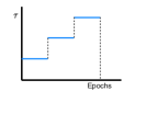
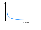
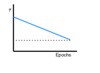
Figure 6: Illustration of the temperature modulation methods: (from left to right) step modulation, exponential modulation, and linear modulation.

Appendix C Additional Results

C.1 Additional Results for 3.2

We demonstrate the tSNE visualization of the features used for OSR and inlier classification to illustrate how feature ensembles affect the separateness of the features. Furthermore, we train and test linear classifiers on top of these features to numerically describe the separateness.

We utilize the features from split 4 in the TinyImagenet protocol as examples and the visualizations are in Figure 7 (For the sake of plotting, the original training dataset is randomly downsampled by $50\%$). The linear classifier is the standard SGDClassifier in sklearn with hinge loss and a fixed number of optimization iterations. We record the testing accuracies, $A_{linear}$, of the linear classifiers and list them in the legends of each feature map.

It is straightforward to find that $A_{linear}$ increases with the increase of the number of ensembles. Furthermore, the ensembles of different temperatures perform better than those with the same temperatures. Ensembling the features with the same temperature can also greatly improve $A_{linear}$. We think it is due to the factor of the randomness in data augmentation and model initialization as well as the richness of the discriminative features. We have tested $A_{linear}$ of the feature ensembles from the same models. their results exhibit no difference from the single model (see Table 8). It can further verify that the models trained using the same temperature can learn various features. We will look into this phenomenon in future work.

$\#$Ensembles	1	2	3
$\tau_{0}$	$90.89\%$	$91.09\%$	$90.94\%$
$\tau_{1}$	$92.33\%$	$91.98\%$	$92.43\%$
$\tau_{2}$	$92.18\%$	$92.03\%$	$92.03\%$

Table 8: $A_{linear}$ of the feature ensembles from the same models tested on TinyImagenet protocol.

However, this natural characteristic of the ensembles doesn’t exist for our SupCon Smooth method with one single model. Hence it is still meaningful to increase the feature diversity through modulating the temperature during training. In future work, we will try to combine these two directions to provide more diverse features for OSR.

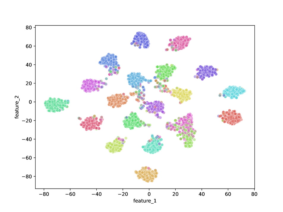
(a) $\tau_{0}$, $A_{linear}=90.89\%$

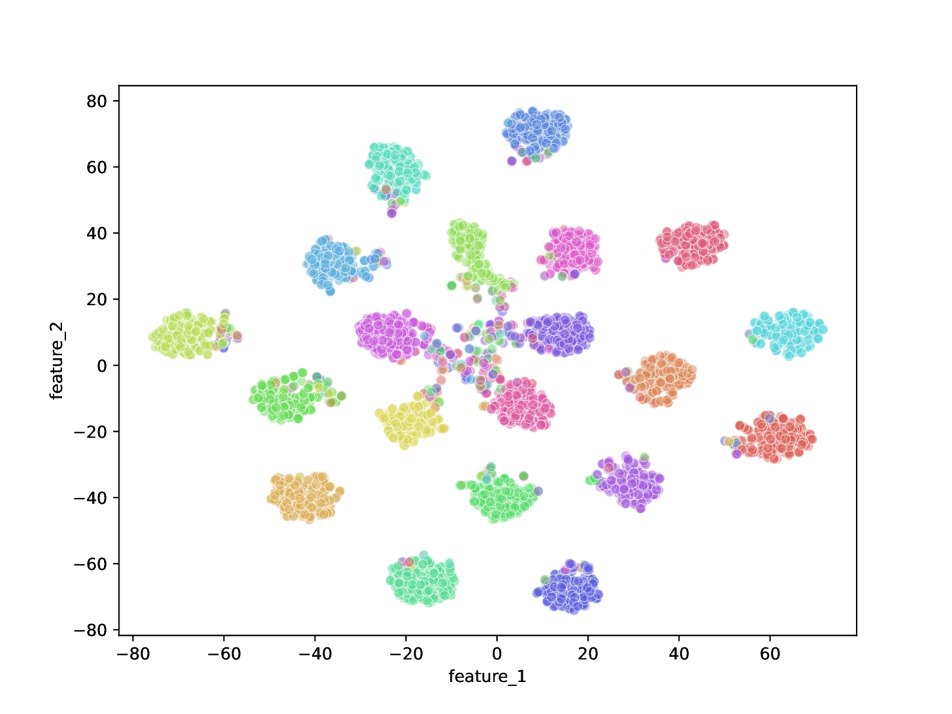
(b) $\tau_{1}$, $A_{linear}=92.33\%$

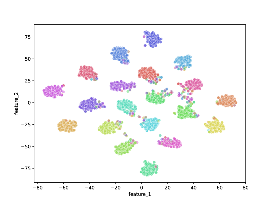
(c) $\tau_{2}$, $A_{linear}=92.18\%$

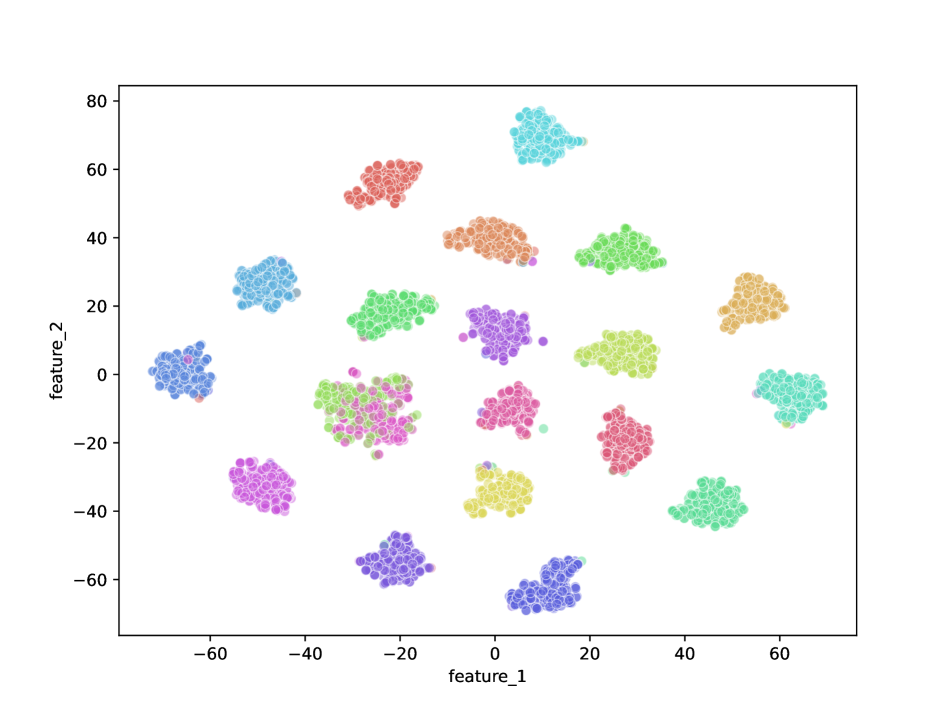
(d) $\tau_{0},\tau_{0}$, $A_{linear}=97.13\%$

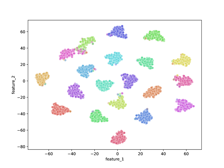
(e) $\tau_{1},\tau_{1}$, $A_{linear}=98.22\%$

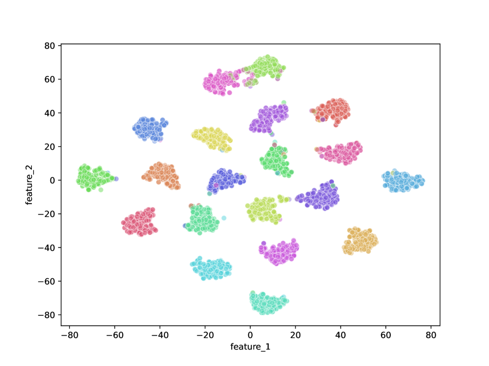
(f) $\tau_{2},\tau_{2}$, $A_{linear}=97.82\%$

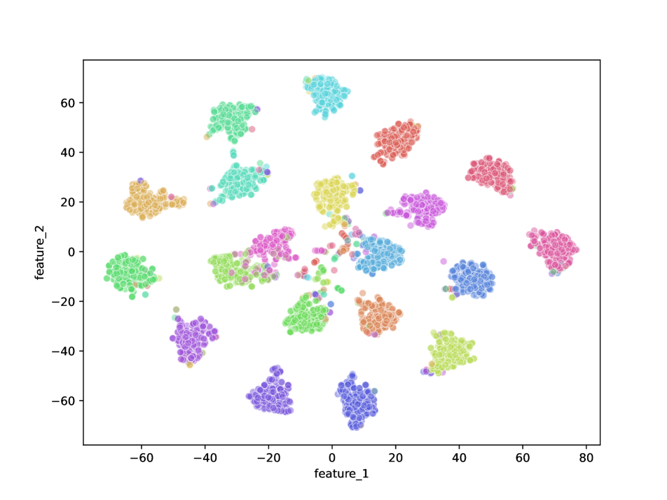
(g) $\tau_{0},\tau_{1}$, $A_{linear}=98.37\%$

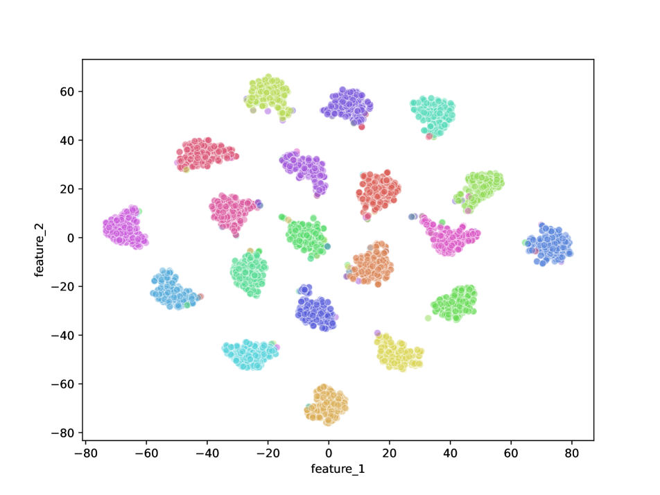
(h) $\tau_{1},\tau_{2}$, $A_{linear}=98.66\%$

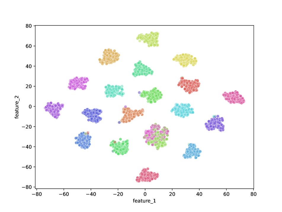
(i) $\tau_{0},\tau_{0},\tau_{0}$, $A_{linear}=97.38\%$

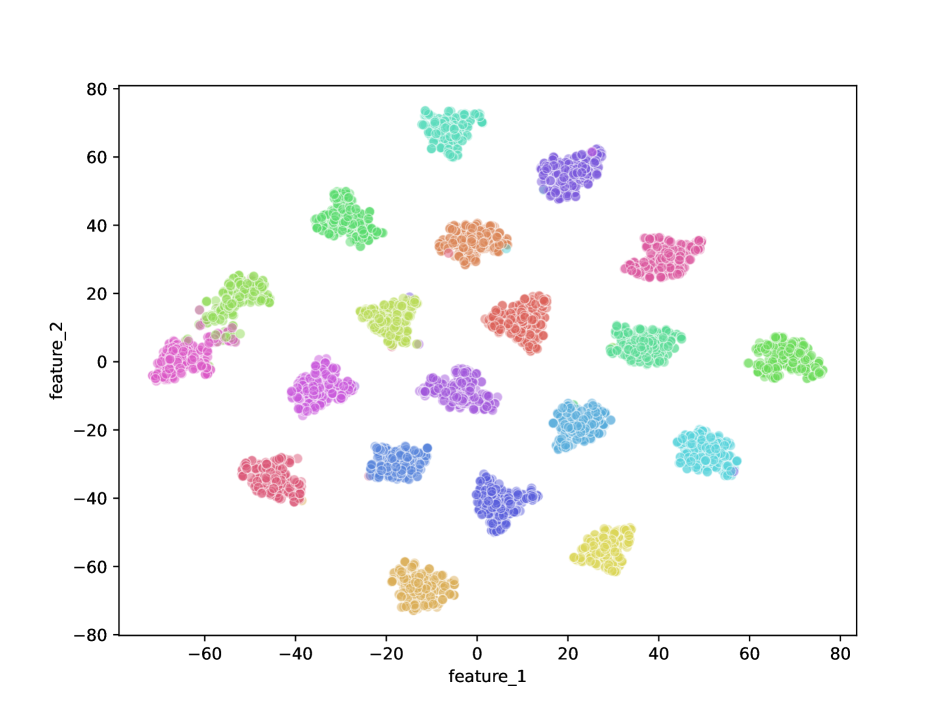
(j) $\tau_{1},\tau_{1},\tau_{1}$, $A_{linear}=98.66\%$

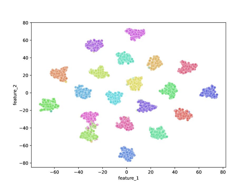
(k) $\tau_{2},\tau_{2},\tau_{2}$, $A_{linear}=97.86\%$

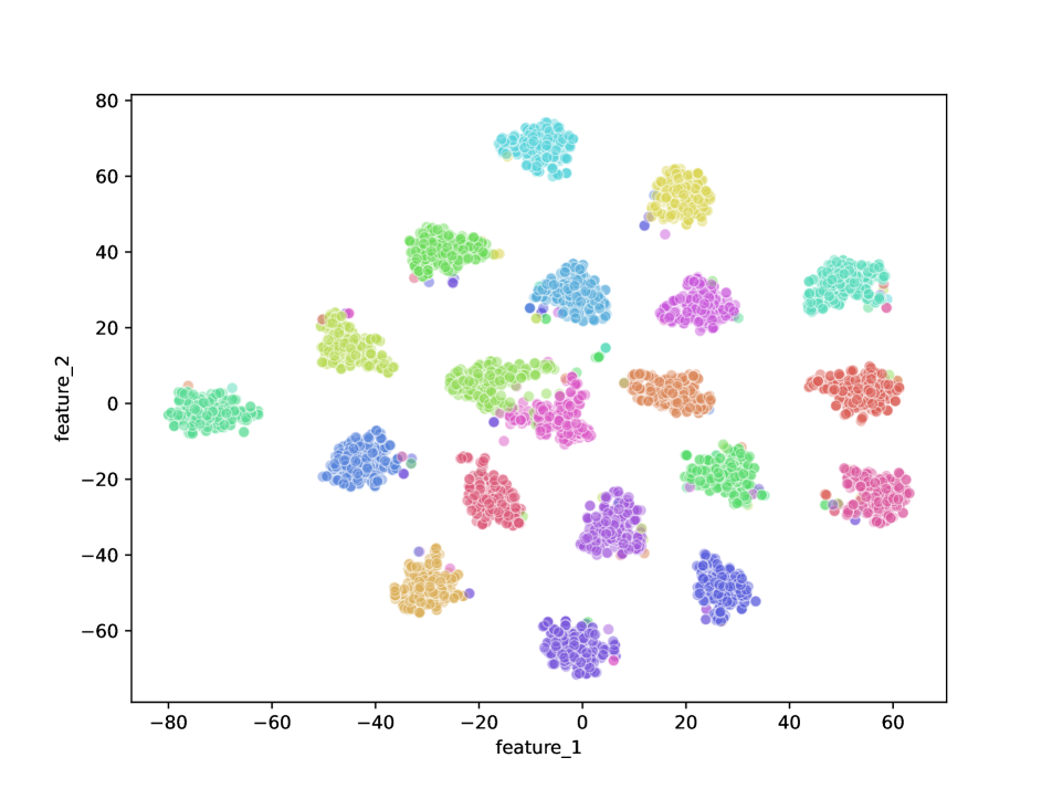
(l) $\tau_{0},\tau_{1},\tau_{2}$, $A_{linear}=99.36\%$

Figure 7: tSNE visualization of the features with variant ensemble settings on TinyImagenet protocol (Better viewed with zoom in and different colors represent different inlier classes).

C.2 Mathematical Derivations in 3.1.2

We give the gradient derivation process in Equation (2) and (3) here:

$$\begin{split}&\frac{\partial\mathcal{L}_{SupCon}}{\partial s_{ip}}\\ &=\frac{\partial\sum\limits_{i\in I}\frac{-1}{|P(i)|}\sum\limits_{p}\left[\frac{s_{ip}}{\tau}-\log[\sum\limits_{p}\exp(\frac{s_{ip}}{\tau})+\sum\limits_{n}\exp(\frac{s_{in}}{\tau})]\right]}{\partial s_{ip}}\\ &\propto-\frac{1}{\tau}+\frac{\frac{1}{\tau}\exp(\frac{s_{ip}}{\tau})}{\sum\limits_{p}\exp(\frac{s_{ip}}{\tau})+\sum\limits_{n}\exp(\frac{s_{in}}{\tau})}\\ &=\frac{1}{\tau}\left[softmax(\frac{s_{ip}}{\tau})-1\right]\end{split}$$ (13)

$$\begin{split}&\frac{\partial\mathcal{L}_{SupCon}}{\partial s_{in}}\\ &=\sum\limits_{i\in I}\frac{1}{|P(i)|}\sum\limits_{p}\frac{\partial\log\left[\sum\limits_{p}\exp(\frac{s_{ip}}{\tau})+\sum\limits_{n}\exp(\frac{s_{in}}{\tau})\right]}{\partial s_{in}}\\ &\propto\frac{\frac{1}{\tau}\exp(\frac{s_{in}}{\tau})}{\sum\limits_{p}\exp(\frac{s_{ip}}{\tau})+\sum\limits_{n}\exp(\frac{s_{in}}{\tau})}\\ &=\frac{1}{\tau}softmax(\frac{s_{in}}{\tau})\end{split}$$ (14)

Appendix D Introduction on Popular OSR Methods (Baselines in Section 5)

Openmax

It has been observed in Openmax that the penultimate layers of deep networks (the fully connected layer before SoftMax) exhibit distinct patterns between different classes. The patterns of the penultimate layers of the correctly classified inliers are modeled using extreme value theory, which is utilized to score the testing samples to detect outliers.

G-Openmax

A generative adversarial network (GAN) is employed on G-openmax to synthesize outliers. The classifier is trained with a mix of the generated outliers and inliers. The OSR framework in G-openmax is the same as in Openmax.

OSRCI

The counterfactual images, i.e., the outliers that look similar to the inliers, are synthesized using GAN in OSRCI. A $N+1$ classifier, where $N$ stands for the number of inlier classes and $1$ represents the outliers, is trained to classify the inliers and detect outliers.

C2AE

A class conditional autoencoder is trained on inliers in CA2E. The reconstruction errors of the inliers are modeled using the extreme value theory, which is utilized to compare with these given by outliers.

ARPL & ARPL+CS

Adversarial reciprocal points learning (ARPL) aims at modeling the outliers through pushing the reciprocal points away from each inlier class. The reciprocal points represent the entire data space except for the current inlier class and are trainable. In its extended version, the confusion samples (CS) are generated using GANs and are applied to train the discriminative models. The confusion samples are those that are semantically similar to the inliers, which is a commonly used strategy introduced in Section 1.

MLS

MLS is no new OSR method, in which the commonly applied strategies for training cross-entropy-based supervised classifiers are heavily applied, i.e., data augmentation, label smoothing, and long training epochs. The method is named MLS for its use of maximum logit score, which takes the norms of the raw outputs of the final linear layer as criteria to detect outliers.

Appendix E Further Discussion

E.1 Feature Forgetting in SupCon

We apply Centred Kernel Alignment (CKA) [25], which is defined as in (15), to measure feature forgetting when training using various temperatures. CKA is a metric to compare the high-dimensional intermediate features in neural networks and invariant to invertible linear and orthogonal transformations that can be applied to compare the features of the same layers in different training stages. In (15), $\mathbf{X}\in\mathbb{R}^{m\times n_{x}}$ and $\mathbf{Y}\in\mathbb{R}^{m\times n_{y}}$ are set of features of dimension $n_{x}$ and $n_{y}$ on the dataset of size $m$ respectively.

$$S_{CKA}=\frac{\|\mathbf{X}^{T}\mathbf{Y}\|_{F}^{2}}{\|\mathbf{Y}^{T}\mathbf{Y}\|_{F}\|\mathbf{X}^{T}\mathbf{X}\|_{F}}$$ (15)

We record $S_{CKA}$ between the features used for OSR from successive epochs when training using step-wise changing temperatures. We set the temperature change among $[0.05,0.049,0.048]$, $[0.05,0.01,0.005]$, $[0.1,0.01,0.005]$ and train the model on top of a pre-trained model with $\tau=0.05$, $\tau=0.05$, $\tau=0.1$ respectively. There are $30$ epochs in total and the temperature changes at epoch $10$ and $20$. We plot $S_{CKA}$ versus the epochs with respect to the above three groups of temperatures, namely $S_{CKA}^{1}$, $S_{CKA}^{2}$, $S_{CKA}^{3}$, in Figure 8. $S_{CKA}^{2}$, $S_{CKA}^{3}$ exhibit a drop when the temperature changes, which indicates a faster feature change than training using very slowly changing temperatures.

Figure 8: Plot of $S_{CKA}^{1}$, $S_{CKA}^{2}$, $S_{CKA}^{3}$, which are the feature similarities between successive epochs during training using step-wise changing temperatures. Red vertical lines indicate the epoch that the temperature changes.

In future work, we will look into the feature forgetting from a semantic perspective. Although slowing the temperature change can reduce forgetting, we will explore more effective ways to let the models preserve the learned features in SupCon models.

References

- Alex et al. [a] K. Alex, N. Vinod, and H. Geoffrey. Cifar-10 (canadian institute for advanced research). a.
- Alex et al. [b] K. Alex, N. Vinod, and H. Geoffrey. Cifar-100 (canadian institute for advanced research). b.
- Bendale and Boult [2016] A. Bendale and T. E. Boult. Towards open set deep networks. In Proceedings of the IEEE Conference on Computer Vision and Pattern Recognition (CVPR’16), pages 1563–1572, 2016.
- Boudiaf et al. [2020] M. Boudiaf, J. Rony, I. M. Ziko, E. Granger, M. Pedersoli, P. Piantanida, and I. B. Ayed. A unifying mutual information view of metric learning: cross-entropy vs. pairwise losses. In European conference on computer vision, pages 548–564. Springer, 2020.
- Cantu-Paz [2004] E. Cantu-Paz. Feature subset selection, class separability, and genetic algorithms. In Genetic and Evolutionary Computation–GECCO 2004: Genetic and Evolutionary Computation Conference, Seattle, WA, USA, June 26-30, 2004. Proceedings, Part I, pages 959–970. Springer, 2004.
- Cao et al. [2021] A. Cao, Y. Luo, and D. Klabjan. Open-set recognition with gaussian mixture variational autoencoders. In Proceedings of the AAAI Conference on Artificial Intelligence, pages 6877–6884, 2021.
- Chapman and Liu [2022] A. Chapman and L. Liu. Regularizing neural network training via identity-wise discriminative feature suppression. In 2022 International Conference on Digital Image Computing: Techniques and Applications (DICTA), pages 1–7. IEEE, 2022.
- Chen et al. [2020a] G. Chen, L. Qiao, Y. Shi, P. Peng, J. Li, T. Huang, S. Pu, and Y. Tian. Learning open set network with discriminative reciprocal points. In Computer Vision–ECCV 2020: 16th European Conference, Glasgow, UK, August 23–28, 2020, Proceedings, Part III 16, pages 507–522. Springer, 2020a.
- Chen et al. [2022] G. Chen, P. Peng, X. Wang, and Y. Tian. Adversarial reciprocal points learning for open set recognition. IEEE Transactions on Pattern Analysis and Machine Intelligence, 2022.
- Chen et al. [2020b] T. Chen, S. Kornblith, M. Norouzi, and G. Hinton. A simple framework for contrastive learning of visual representations. In International conference on machine learning, pages 1597–1607. PMLR, 2020b.
- Deng et al. [2009] J. Deng, W. Dong, R. Socher, L.-J. Li, K. Li, and L. Fei-Fei. Imagenet: A large-scale hierarchical image database. In 2009 IEEE Conference on Computer Vision and Pattern Recognition (CVPR’09), pages 248–255. IEEE, 2009.
- Deng [2012] L. Deng. The mnist database of handwritten digit images for machine learning research. IEEE Signal Processing Magazine, 29(6):141–142, 2012.
- Dhamija et al. [2018] A. R. Dhamija, M. Günther, and T. Boult. Reducing network agnostophobia. Advances in Neural Information Processing Systems, 31, 2018.
- Ge et al. [2017] Z. Ge, S. Demyanov, and R. Garnavi. Generative openmax for multi-class open set classification. In British Machine Vision Conference 2017 (BMVC’17), London, UK, 2017.
- Geirhos et al. [2020] R. Geirhos, J.-H. Jacobsen, C. Michaelis, R. Zemel, W. Brendel, M. Bethge, and F. A. Wichmann. Shortcut learning in deep neural networks. Nature Machine Intelligence, 2(11):665–673, 2020.
- Hassen and Chan [2020] M. Hassen and P. K. Chan. Learning a neural-network-based representation for open set recognition. In Proceedings of the 2020 SIAM International Conference on Data Mining, pages 154–162. SIAM, 2020.
- He et al. [2016] K. He, X. Zhang, S. Ren, and J. Sun. Deep residual learning for image recognition. In Proceedings of the IEEE conference on computer vision and pattern recognition, pages 770–778, 2016.
- Jiang et al. [2020] Z. Jiang, T. Chen, T. Chen, and Z. Wang. Robust pre-training by adversarial contrastive learning. Advances in neural information processing systems, 33:16199–16210, 2020.
- Kamoi and Kobayashi [2020] R. Kamoi and K. Kobayashi. Why is the mahalanobis distance effective for anomaly detection? arXiv preprint arXiv:2003.00402, 2020.
- Karpathy et al. [2014] A. Karpathy, G. Toderici, S. Shetty, T. Leung, R. Sukthankar, and L. Fei-Fei. Large-scale video classification with convolutional neural networks. In Proceedings of the IEEE conference on Computer Vision and Pattern Recognition, pages 1725–1732, 2014.
- Kaya and Bilge [2019] M. Kaya and H. Ş. Bilge. Deep metric learning: A survey. Symmetry, 11(9):1066, 2019.
- Khan et al. [2022] S. S. Khan, Z. Shen, H. Sun, A. Patel, and A. Abedi. Supervised contrastive learning for detecting anomalous driving behaviours from multimodal videos. In 2022 19th Conference on Robots and Vision (CRV), pages 16–23. IEEE, 2022.
- Khosla et al. [2020] P. Khosla, P. Teterwak, C. Wang, A. Sarna, Y. Tian, P. Isola, A. Maschinot, C. Liu, and D. Krishnan. Supervised contrastive learning. Advances in neural information processing systems, 33:18661–18673, 2020.
- Kingma and Ba [2014] D. P. Kingma and J. Ba. Adam: A method for stochastic optimization. arXiv preprint arXiv:1412.6980, 2014.
- Kornblith et al. [2019] S. Kornblith, M. Norouzi, H. Lee, and G. Hinton. Similarity of neural network representations revisited. In International conference on machine learning, pages 3519–3529. PMLR, 2019.
- Kukleva et al. [2022] A. Kukleva, M. Böhle, B. Schiele, H. Kuehne, and C. Rupprecht. Temperature schedules for self-supervised contrastive methods on long-tail data. In The Eleventh International Conference on Learning Representations, 2022.
- Lee et al. [2018] K. Lee, K. Lee, H. Lee, and J. Shin. A simple unified framework for detecting out-of-distribution samples and adversarial attacks. Advances in neural information processing systems, 31, 2018.
- Lei et al. [2020] Y. Lei, B. Yang, X. Jiang, F. Jia, N. Li, and A. K. Nandi. Applications of machine learning to machine fault diagnosis: A review and roadmap. Mechanical Systems and Signal Processing, 138:106587, 2020.
- Liu et al. [2020] B. Liu, H. Kang, H. Li, G. Hua, and N. Vasconcelos. Few-shot open-set recognition using meta-learning. In Proceedings of the IEEE/CVF Conference on Computer Vision and Pattern Recognition, pages 8798–8807, 2020.
- Michael and Lin [1973] M. Michael and W.-C. Lin. Experimental study of information measure and inter-intra class distance ratios on feature selection and orderings. IEEE Transactions on Systems, Man, and Cybernetics, (2):172–181, 1973.
- Miller et al. [2021] D. Miller, N. Suenderhauf, M. Milford, and F. Dayoub. Class anchor clustering: A loss for distance-based open set recognition. In Proceedings of the IEEE/CVF Winter Conference on Applications of Computer Vision (WACV’21), pages 3570–3578, 2021.
- Mitrovic et al. [2020] J. Mitrovic, B. McWilliams, J. Walker, L. Buesing, and C. Blundell. Representation learning via invariant causal mechanisms. arXiv preprint arXiv:2010.07922, 2020.
- Müller et al. [2019] R. Müller, S. Kornblith, and G. E. Hinton. When does label smoothing help? Advances in neural information processing systems, 32, 2019.
- Narkhede [2018] S. Narkhede. Understanding auc-roc curve. Towards Data Science, 26(1):220–227, 2018.
- Neal et al. [2018] L. Neal, M. Olson, X. Fern, W.-K. Wong, and F. Li. Open set learning with counterfactual images. In Proceedings of the European Conference on Computer Vision (ECCV’18), pages 613–628, 2018.
- Netzer et al. [2011] Y. Netzer, T. Wang, A. Coates, A. Bissacco, B. Wu, and A. Y.Ng. Street view hause number dataset. http://ufldl.stanford.edu/housenumbers, 2011.
- Oord et al. [2018] A. v. d. Oord, Y. Li, and O. Vinyals. Representation learning with contrastive predictive coding. arXiv preprint arXiv:1807.03748, 2018.
- Oza and Patel [2019] P. Oza and V. M. Patel. C2ae: Class conditioned auto-encoder for open-set recognition. In Proceedings of the IEEE/CVF Conference on Computer Vision and Pattern Recognition, pages 2307–2316, 2019.
- Perera et al. [2020] P. Perera, V. I. Morariu, R. Jain, V. Manjunatha, C. Wigington, V. Ordonez, and V. M. Patel. Generative-discriminative feature representations for open-set recognition. In Proceedings of the IEEE/CVF Conference on Computer Vision and Pattern Recognition, pages 11814–11823, 2020.
- Purushwalkam and Gupta [2020] S. Purushwalkam and A. Gupta. Demystifying contrastive self-supervised learning: Invariances, augmentations and dataset biases. Advances in Neural Information Processing Systems, 33:3407–3418, 2020.
- Robinson et al. [2020] J. Robinson, C.-Y. Chuang, S. Sra, and S. Jegelka. Contrastive learning with hard negative samples. arXiv preprint arXiv:2010.04592, 2020.
- Robinson et al. [2021] J. Robinson, L. Sun, K. Yu, K. Batmanghelich, S. Jegelka, and S. Sra. Can contrastive learning avoid shortcut solutions? Advances in neural information processing systems, 34:4974–4986, 2021.
- Scheirer et al. [2012] W. J. Scheirer, A. de Rezende Rocha, A. Sapkota, and T. E. Boult. Toward open set recognition. IEEE transactions on pattern analysis and machine intelligence, 35(7):1757–1772, 2012.
- Schölkopf et al. [2021] B. Schölkopf, F. Locatello, S. Bauer, N. R. Ke, N. Kalchbrenner, A. Goyal, and Y. Bengio. Toward causal representation learning. Proceedings of the IEEE, 109(5):612–634, 2021.
- Shen et al. [2022] R. Shen, S. Bubeck, and S. Gunasekar. Data augmentation as feature manipulation. In International conference on machine learning, pages 19773–19808. PMLR, 2022.
- Vaze et al. [2022] S. Vaze, K. Han, A. Vedaldi, and A. Zisserman. Open-set recognition: a good closed-set classifier is all you need? In International Conference on Learning Representations (ICLR’22), 2022.
- Wang and Liu [2021] F. Wang and H. Liu. Understanding the behaviour of contrastive loss. In Proceedings of the IEEE/CVF conference on computer vision and pattern recognition, pages 2495–2504, 2021.
- Wang et al. [2022] Z. Wang, Q. Xu, Z. Yang, Y. He, X. Cao, and Q. Huang. Openauc: Towards auc-oriented open-set recognition. Advances in Neural Information Processing Systems, 35:25033–25045, 2022.
- Yang et al. [2020] H.-M. Yang, X.-Y. Zhang, F. Yin, Q. Yang, and C.-L. Liu. Convolutional prototype network for open set recognition. IEEE Transactions on Pattern Analysis and Machine Intelligence, 44(5):2358–2370, 2020.
- Yoshihashi et al. [2019] R. Yoshihashi, W. Shao, R. Kawakami, S. You, M. Iida, and T. Naemura. Classification-reconstruction learning for open-set recognition. In Proceedings of the IEEE/CVF Conference on Computer Vision and Pattern Recognition, pages 4016–4025, 2019.
- Yu et al. [2017] Y. Yu, W.-Y. Qu, N. Li, and Z. Guo. Open category classification by adversarial sample generation. In International Joint Conference on Artificial Intelligence (IJCAI’17), pages 3357–3363, Melbourne, Australia, 2017.
- Zeng et al. [2021] Z. Zeng, K. He, Y. Yan, Z. Liu, Y. Wu, H. Xu, H. Jiang, and W. Xu. Modeling discriminative representations for out-of-domain detection with supervised contrastive learning. arXiv preprint arXiv:2105.14289, 2021.
- Zhang et al. [2020] H. Zhang, A. Li, J. Guo, and Y. Guo. Hybrid models for open set recognition. In Computer Vision–ECCV 2020: 16th European Conference, Glasgow, UK, August 23–28, 2020, Proceedings, Part III 16, pages 102–117. Springer, 2020.
- Zhang et al. [2018] L. Zhang, S. Wang, and B. Liu. Deep learning for sentiment analysis: A survey. Wiley Interdisciplinary Reviews: Data Mining and Knowledge Discovery, 8(4):e1253, 2018.