Experimental entanglement entropy without twin copy
Abstract
We show that it is possible to estimate experimentally the von Neuman entanglement entropy of a symmetric bi-partite quantum system by using the basic measurement counts for a single copy of a prepared state. We use the entropy associated with the experimental measurements for this state and the reduced entropy obtained by tracing the experimental probabilities over the half of the system. We conjecture that and demonstrate that it is verified in good approximation using exact diagonalization and analog calculations performed with the publicly available QuEra facilities for chains and ladders of Rydberg atoms. The approximate proportionality constant is of order one for the examples considered. can be calculated easily for many other qubit platforms and appears to be generically robust under measurement errors, although a general proof remains to be found. Similar results are found for the second order Rényi entanglement entropy.
Motivations. Entanglement entropy is a crucial theoretical concept in quantum physics with applications for many-body physics Amico et al. (2008); Eisert et al. (2010); Abanin et al. (2019); Cirac et al. (2021), gauge theory Ghosh et al. (2015); Van Acoleyen et al. (2016); Bañuls et al. (2017); Knaute et al. (2024), high-energy collisions Kharzeev and Levin (2017); Baker and Kharzeev (2018); Zhang et al. (2022), nuclear physics Beane et al. (2019); Robin et al. (2021) and studies of conformal field theory Vidal et al. (2003); Korepin (2004); Calabrese and Cardy (2006); Ryu and Takayanagi (2006). It provides important information regarding quantum phases transitions.
However, the experimental measurement of entanglement entropy is notoriously difficult due to its
nonlocal nature.
It has been proposed to measure the entanglement entropy by using a two-level system coupled to several
copies of the original system Abanin and Demler (2012) or the second order Rényi entropy by performing a swap operation between twin copies of a system Daley et al. (2012). Cold atom experimentalists Islam et al. (2015); Kaufman et al. (2016) were able to prepare and interfere
twin copies of a state in small optical lattices to directly measure . If practically feasible on larger systems, this could allow the experimental measurement of the central charge for conformal systems Unmuth-Yockey et al. (2017).
Bitstring probabilities. Preparing and interfering twin copies of a quantum system are not easy experimental tasks. On the other hand, a generic qubit based quantum computing device provides experimental counts for bitstrings which can be used to estimate probabilities associated with measurements in the computational basis. These counts are typically provided as python dictionaries. For instance, {’01’: 269, ’00’: 251, ’10’: 247, ’11’: 233} for a two-qubit universal quantum computer and {’gggrgrgrgr’: 8, ’rgrgrggrgr’: 160, ...} for a 10 Rydberg atom analog simulator where and represent, for each atom, the ground and Rydberg states respectively. By dividing these counts by the total number of shots, we obtain empirical probabilities associated with the bitstring states .
Bipartite setup. We consider a bipartite quantum system made out of two parts and . For simplicity, we assume that and have the same size and can be interchanged by a reflection symmetry. We define the usual Shannon entropy associated with the experimental probabilities as:
| (1) |
As explained in a more systematic way in Supp. Mat. A, we assume that the computational basis has a bipartite factorization and that we can define reduced probabilities by tracing over one half of the system:
| (2) |
This leads to the reduced entropy
| (3) |
An educated guess. It is straightforward to calculate and from output dictionaries but these quantities depend strongly on the computational basis and do not provide unique characterizations of the the system. On the other hand, given our assumptions, we see that for a uniform product state . We guessed that the difference between these two quantities could be used to estimate the basis-independent entanglement between and .
Main results. In the following we will consider a pure state density matrix for the vacuum and its reduced density matrix with the standard von Neumann entanglement entropy
| (4) |
which is independent of the basis used. We will show with some examples that in good approximation
| (5) |
and that, as guessed, basis-dependent features as well as measurement errors tend to cancel in this specific linear combination. Experimental probabilities for a single copy are available on many analog and universal quantum computing platforms. In the following, we focus on configurable arrays of Rydberg atoms. We conducted experimental analog simulations using the QuEra device Aquila Wurtz et al. (2023) which is publicly available. Rydberg atoms setup. Recently, arrays of optical tweezer have been used to create arrays of Rydberg atoms with adjustable geometries Bernien et al. (2017); Keesling et al. (2019); Labuhn et al. (2016); de Léséleuc et al. (2019); Ebadi et al. (2021); Scholl et al. (2021). Their Hamiltonian reads
| (6) |
with van der Waals interactions , for a distance between the atoms labelled as and . By definition, , the Rydberg blockade radius, when the Rabi frequency. We define the Rydberg occupation while . In the following we use MHz, which implies , and a detuning MHz. We will consider chains and ladders of atoms with varying lattice spacings.
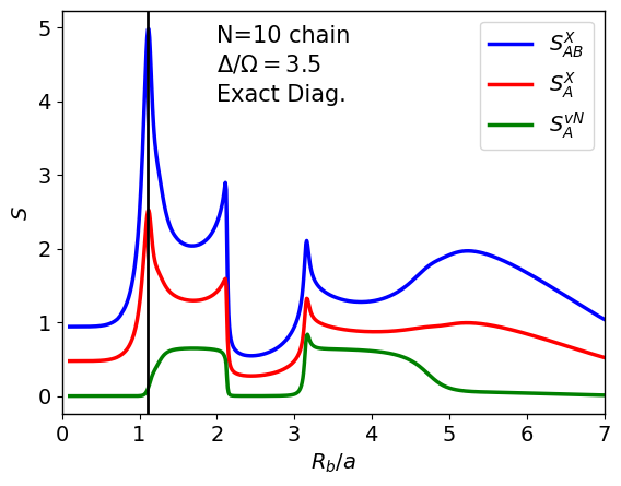
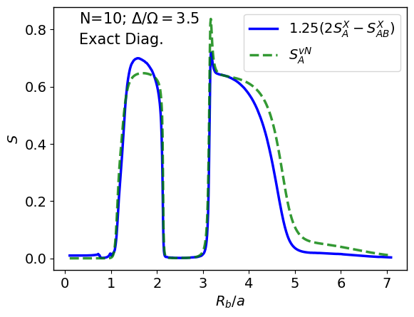
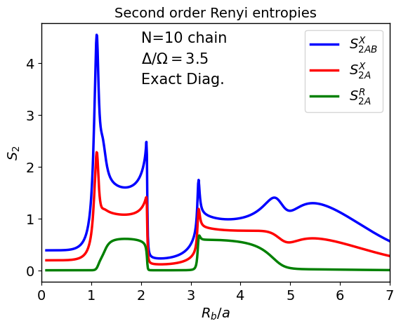
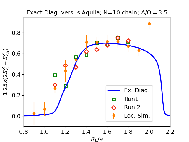
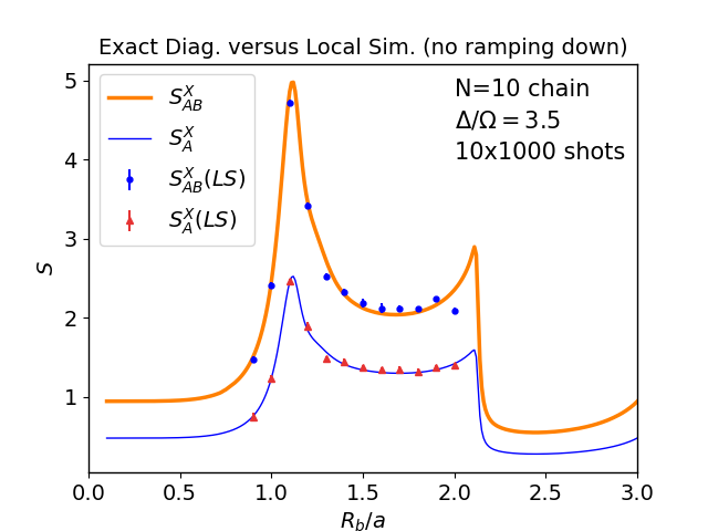
Numerical calculations. A first illustration of Eq. (5) is obtained by using the ground state of a chain of 10 Rydberg atoms separated by a varied lattice spacing expressed in units of . We used exact diagonalization to calculate , and for the vacuum. The results are shown in Fig. 1. We observe that . The proportionality is only approximate, for instance, is slightly below (above) this linear combination for smaller (larger) respectively. Notice that as is increased from low values, the onset of is marked by a sharp increase and . However, at the peak of and , cancellations occur and develops only after and drop significantly. Other features of Fig. 1 can be understood from elementary considerations that are provided in Supp. Mat. B.
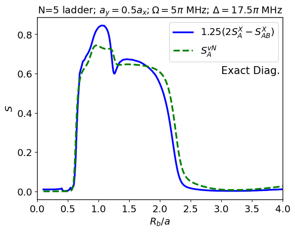
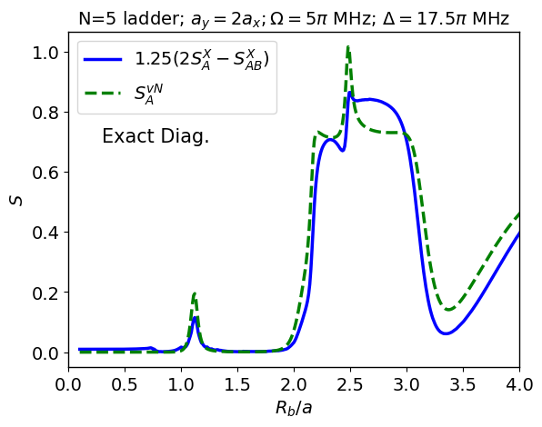
Other numerical examples. It is easy to illustrate Eq. (5) with other geometries. We have considered two-leg ladders with five rungs and varied lattice spacing in both directions. We observed similar features shown in Supp. Mat. C. Again the approximate constant of proportionality 1.25 was used to display both quantities in the same figure. Other values of the constant need to be used for other systems with less atoms and 1.25 does no seem to have any universal meaning.
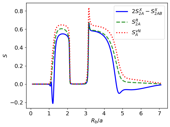
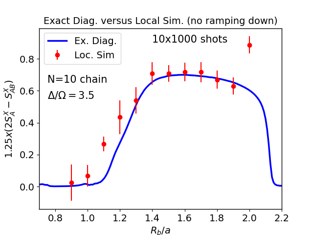
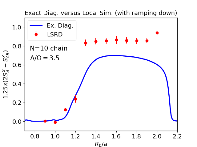
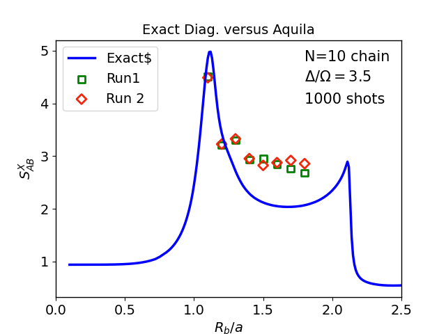
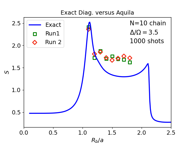
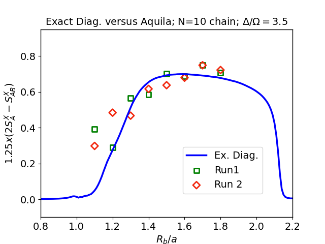
Analog calculations. We have repeated the single chain calculation with 10 atoms and the same and as before, using the Aquila device and the associated AWS Braket local simulator. In both cases, we ramped up the vacuum adiabatically with size constraints not present in exact diagonalization. Calculations for can be performed with the local simulator and for a slightly shorter range of with Aquila. Practical aspects are discussed in Supp. Mat. D. The ramping down of for measurements at the end involves subtleties discussed in Supp. Mat. E. The results are shown in Fig. 2 where we see good estimates of , and consequently of , with both procedures. This figure is the main result presented here.
Error cancellations. An important aspect of the results presented in Fig. 2 is that the systematic errors of and are significant. However these errors appear to cancel in . This is discussed in Supp. Mat. E. Note that we do not attempt to understand the nature of these errors here but only notice their approximate cancellations. Applications. Arrays of Rydberg atoms have been proposed for quantum simulation of lattice gauge theories Zhang et al. (2018); Surace et al. (2020); Notarnicola et al. (2020); Celi et al. (2020); Meurice (2021); Fromholz et al. (2022); González-Cuadra et al. (2022); Heitritter et al. (2022). More specifically, ladder arrays have been considered as quantum simulators for scalar electrodynamics Meurice (2021) and their phase diagram have been studied experimentally Zhang et al. (2024) and with effective Hamiltonian methods Zhang et al. (2023). These results show a very rich phase diagram and the need to study the regions of parameter spaces where the correlation lengths are much larger than the lattice spacing with possible relevance for the study of inhomogeneous phases and the Lifshitz regime of lattice quantum chromodynamics Pisarski et al. (2019); Kojo et al. (2010). Entanglement entropy considerations play an important role in the tentative designs of hybrid algorithm for collider event generators Heitritter et al. (2022). The method proposed here could be crucial to study extended two-dimensional arrays with possibly a small third dimension in the future. Generalizations. So far Eq. (5) has been an unexpectedly successful guess. Fig. 1 shows clearly the approximate factor 2 relating the height of the peaks of and . In between the peaks, the changes can be estimated in terms of the bitstring distribution, however we do not have a general argument supporting Eq. (5). The connection between correlations and purity Lukin et al. (2019) or the reconstruction of quantum states using a restricted Boltzmann machine based on single-basis measurements Torlai et al. (2019) could help develop a more general undestanding. Another more general perspective can be found in Ref. Zhang et al. (2024), where one can see precise correspondence in the contour plots of the peak height of the structure factors, which can be reconstructed for the only, and . This makes clear that the contain all the information necessary to reconstruct .
Rényi entropy. One can easily construct a second order Rényi version of the von Neumann quantities defined above:
| (7) |
As shown in Supp.Mat. F, we found a very similar result for the 10 atom chain using exact diagonalization:
| (8) |
with . In addition, we found that and similar constants of proportionality. Conclusions. We have provided three Rydberg array examples where the von Neumann entanglement entropy can be estimated in good approximation from . This quantity was picked by considering limits and looking at the heights of the peaks in Fig. 1 but we do not have a general proof that it is proportional to . This quantity can be calculated easily using the bitstring probabilities for a single copy and seems to be robust against systematic errors. The method can be applied to any qubit based universal or analog quantum computing device and we hope that this can lead to a broader set of supporting evidence for our observation.
Acknowledgements
This research was supported in part by the Dept. of Energy under Award Number DE-SC0019139. We thank S. Cantu, M. Asaduzzaman, J. Corona, Cheng Chin, Sheng-Tao Wang, A. Bylinskii, Fangli Liu, J. Zeiher and R. Pisarski for comments and support. We thank the Amazon Web Services and S. Hassinger for facilitating remote access to QuEra through the Amazon Braket while teaching quantum mechanics and our Department of Physics and Astronomy for supporting the analog simulations presented here.
References
- Amico et al. (2008) L. Amico, R. Fazio, A. Osterloh, and V. Vedral, Reviews of modern physics 80, 517 (2008).
- Eisert et al. (2010) J. Eisert, M. Cramer, and M. B. Plenio, Rev. Mod. Phys. 82, 277 (2010), arXiv:0808.3773 [quant-ph] .
- Abanin et al. (2019) D. A. Abanin, E. Altman, I. Bloch, and M. Serbyn, Reviews of Modern Physics 91 (2019), 10.1103/revmodphys.91.021001.
- Cirac et al. (2021) J. I. Cirac, D. Perez-Garcia, N. Schuch, and F. Verstraete, Rev. Mod. Phys. 93, 045003 (2021), arXiv:2011.12127 [quant-ph] .
- Ghosh et al. (2015) S. Ghosh, R. M. Soni, and S. P. Trivedi, JHEP 09, 069 (2015), arXiv:1501.02593 [hep-th] .
- Van Acoleyen et al. (2016) K. Van Acoleyen, N. Bultinck, J. Haegeman, M. Marien, V. B. Scholz, and F. Verstraete, Phys. Rev. Lett. 117, 131602 (2016), arXiv:1511.04369 [quant-ph] .
- Bañuls et al. (2017) M. C. Bañuls, K. Cichy, J. I. Cirac, K. Jansen, and S. Kühn, Phys. Rev. X 7, 041046 (2017), arXiv:1707.06434 [hep-lat] .
- Knaute et al. (2024) J. Knaute, M. Feuerstein, and E. Zohar, JHEP 02, 174 (2024), arXiv:2401.01930 [quant-ph] .
- Kharzeev and Levin (2017) D. E. Kharzeev and E. M. Levin, Phys. Rev. D 95, 114008 (2017), arXiv:1702.03489 [hep-ph] .
- Baker and Kharzeev (2018) O. K. Baker and D. E. Kharzeev, Phys. Rev. D 98, 054007 (2018).
- Zhang et al. (2022) K. Zhang, K. Hao, D. Kharzeev, and V. Korepin, Phys. Rev. D 105, 014002 (2022), arXiv:2110.04881 [quant-ph] .
- Beane et al. (2019) S. R. Beane, D. B. Kaplan, N. Klco, and M. J. Savage, Phys. Rev. Lett. 122, 102001 (2019), arXiv:1812.03138 [nucl-th] .
- Robin et al. (2021) C. Robin, M. J. Savage, and N. Pillet, Phys. Rev. C 103, 034325 (2021), arXiv:2007.09157 [nucl-th] .
- Vidal et al. (2003) G. Vidal, J. I. Latorre, E. Rico, and A. Kitaev, Phys. Rev. Lett. 90, 227902 (2003).
- Korepin (2004) V. E. Korepin, Phys. Rev. Lett. 92, 096402 (2004).
- Calabrese and Cardy (2006) P. Calabrese and J. L. Cardy, Int. J. Quant. Inf. 4, 429 (2006), arXiv:quant-ph/0505193 .
- Ryu and Takayanagi (2006) S. Ryu and T. Takayanagi, Phys. Rev. Lett. 96, 181602 (2006), arXiv:hep-th/0603001 .
- Abanin and Demler (2012) D. A. Abanin and E. Demler, Phys. Rev. Lett. 109, 020504 (2012).
- Daley et al. (2012) A. J. Daley, H. Pichler, J. Schachenmayer, and P. Zoller, Phys. Rev. Lett. 109, 020505 (2012).
- Islam et al. (2015) R. Islam, R. Ma, P. M. Preiss, M. E. Tai, A. Lukin, M. Rispoli, and M. Greiner, (2015), 10.1038/nature15750, arXiv:1509.01160 [cond-mat.quant-gas] .
- Kaufman et al. (2016) A. M. Kaufman, M. E. Tai, A. Lukin, M. Rispoli, R. Schittko, P. M. Preiss, and M. Greiner, Science 353, aaf6725 (2016).
- Unmuth-Yockey et al. (2017) J. Unmuth-Yockey, J. Zhang, P. M. Preiss, L.-P. Yang, S. W. Tsai, and Y. Meurice, Phys. Rev. A 96, 023603 (2017), arXiv:1611.05016 [cond-mat.quant-gas] .
- Wurtz et al. (2023) J. Wurtz, A. Bylinskii, B. Braverman, J. Amato-Grill, S. H. Cantu, F. Huber, A. Lukin, F. Liu, P. Weinberg, J. Long, S.-T. Wang, N. Gemelke, and A. Keesling, “Aquila: Quera’s 256-qubit neutral-atom quantum computer,” (2023), arXiv:2306.11727 [quant-ph] .
- Bernien et al. (2017) H. Bernien, S. Schwartz, A. Keesling, H. Levine, A. Omran, H. Pichler, S. Choi, A. S. Zibrov, M. Endres, M. Greiner, V. Vuletić, and M. D. Lukin, Nature 551, 579 (2017).
- Keesling et al. (2019) A. Keesling, A. Omran, H. Levine, H. Bernien, H. Pichler, S. Choi, R. Samajdar, S. Schwartz, P. Silvi, S. Sachdev, P. Zoller, M. Endres, M. Greiner, V. Vuletić, and M. D. Lukin, Nature 568, 207 (2019).
- Labuhn et al. (2016) H. Labuhn, D. Barredo, S. Ravets, S. de Léséleuc, T. Macrì, T. Lahaye, and A. Browaeys, Nature 534, 667 (2016).
- de Léséleuc et al. (2019) S. de Léséleuc, V. Lienhard, P. Scholl, D. Barredo, S. Weber, N. Lang, H. P. Büchler, T. Lahaye, and A. Browaeys, Science 365, 775 (2019).
- Ebadi et al. (2021) S. Ebadi, T. T. Wang, H. Levine, A. Keesling, G. Semeghini, A. Omran, D. Bluvstein, R. Samajdar, H. Pichler, W. W. Ho, S. Choi, S. Sachdev, M. Greiner, V. Vuletić, and M. D. Lukin, Nature 595, 227 (2021).
- Scholl et al. (2021) P. Scholl, M. Schuler, H. J. Williams, A. A. Eberharter, D. Barredo, K.-N. Schymik, V. Lienhard, L.-P. Henry, T. C. Lang, T. Lahaye, A. M. Läuchli, and A. Browaeys, Nature 595, 233 (2021).
- Zhang et al. (2018) J. Zhang, J. Unmuth-Yockey, J. Zeiher, A. Bazavov, S.-W. Tsai, and Y. Meurice, Phys. Rev. Lett. 121, 223201 (2018).
- Surace et al. (2020) F. M. Surace, P. P. Mazza, G. Giudici, A. Lerose, A. Gambassi, and M. Dalmonte, Phys. Rev. X 10, 021041 (2020).
- Notarnicola et al. (2020) S. Notarnicola, M. Collura, and S. Montangero, Phys. Rev. Res. 2, 013288 (2020).
- Celi et al. (2020) A. Celi, B. Vermersch, O. Viyuela, H. Pichler, M. D. Lukin, and P. Zoller, Phys. Rev. X 10, 021057 (2020), arXiv:1907.03311 [quant-ph] .
- Meurice (2021) Y. Meurice, Phys. Rev. D 104, 094513 (2021), arXiv:2107.11366 [quant-ph] .
- Fromholz et al. (2022) P. Fromholz, M. Tsitsishvili, M. Votto, M. Dalmonte, A. Nersesyan, and T. Chanda, Phys. Rev. B 106, 155411 (2022).
- González-Cuadra et al. (2022) D. González-Cuadra, T. V. Zache, J. Carrasco, B. Kraus, and P. Zoller, Phys. Rev. Lett. 129, 160501 (2022), arXiv:2203.15541 [quant-ph] .
- Heitritter et al. (2022) K. Heitritter, Y. Meurice, and S. Mrenna, (2022), arXiv:2212.02476 [quant-ph] .
- Zhang et al. (2024) J. Zhang, S. H. Cantú, F. Liu, A. Bylinskii, B. Braverman, F. Huber, J. Amato-Grill, A. Lukin, N. Gemelke, A. Keesling, S.-T. Wang, Y. Meurice, and S. W. Tsai, “Probing quantum floating phases in rydberg atom arrays,” (2024), arXiv:2401.08087 [quant-ph] .
- Zhang et al. (2023) J. Zhang, S.-W. Tsai, and Y. Meurice, (2023), arXiv:2312.04436 [quant-ph] .
- Pisarski et al. (2019) R. D. Pisarski, V. V. Skokov, and A. M. Tsvelik, Universe 5, 48 (2019).
- Kojo et al. (2010) T. Kojo, Y. Hidaka, L. McLerran, and R. D. Pisarski, Nuclear Physics A 843, 37 (2010).
- Lukin et al. (2019) A. Lukin, M. Rispoli, R. Schittko, M. E. Tai, A. M. Kaufman, S. Choi, V. Khemani, J. Léonard, and M. Greiner, Science 364, 256–260 (2019).
- Torlai et al. (2019) G. Torlai, B. Timar, E. P. van Nieuwenburg, H. Levine, A. Omran, A. Keesling, H. Bernien, M. Greiner, V. Vuletić, M. D. Lukin, R. G. Melko, and M. Endres, Physical Review Letters 123 (2019), 10.1103/physrevlett.123.230504.
SUPPLEMENTAL MATERIAL
Appendix A Bi-partite Hilbert space
In the following we consider two-state systems (qubits), for instance an array of Rydberg atoms either in the ground or Rydberg state. For simplicity, we assume that is even and that the whole system () can be divided in two subsystems and that can be mapped into each other by some reflection symmetry. A simple example is a linear chain of equally spaced Rydberg atoms with an even number of atoms.
The computational basis consists of the elements
| (9) |
Any element of this basis can be factored in a bi-partite way with the two subsystems of identical size A and B (each with qubits)
| (10) |
with
| (11) | |||||
| (12) |
Given an arbitrary prepared state , we can expand it in the computational basis
| (13) |
This implies that the state will be observed with a probability
| (14) |
These probabilities can be estimated by measurements and define an “experimental” entropy
| (15) |
associated with the state . It is clear that this quantity depends on the computational basis and that it contains no information about entanglement.
We now define a reduced probability in the subsystem by tracing over :
| (16) |
and the corresponding reduced entropy
| (17) |
Again, this quantity depend on the computational basis used and cannot be identified with the von Neuman entropy .
In the following we focus on the case where , the vacuum of the Hamiltonian. Starting with
| (18) |
and writing the dimensional vector corresponding to the vacuum as a matrix
| (19) |
we find that the reduced density matrix can be written as
| (20) |
in the computational basis. The von Neuman entropy is
| (21) |
with the eigenvalues of which are independent of the basis used.
Appendix B Detailed features of Fig. 1
Several features of Fig. 1 can be understood from elementary considerations. For , we have essentially 10 decoupled atoms. Each of the single-atom ground states have a probability (with ) to be in the state and the entropy per atom is 0.0951. Numerically we found with 3 significant digits while is negligible. Near =1, and increase rapidly to reach maxima near with . The most probable state is with a probability of 0.036. For , there are four states with probablities larger than 0.1: . (0.138) and (0.276). After tracing over the right part, there are three significant probabilities for , , and and while . For , the state has a probability 0.888 and both and are small.
Appendix C Other examples
We repeated the calculation for ladder-shaped arrays with 5 rungs and 2 legs and different aspect ratios. We found very similar results for the same approximate constant 1.25 as shown in Fig. 3.
Appendix D Practical aspects of analog simulations
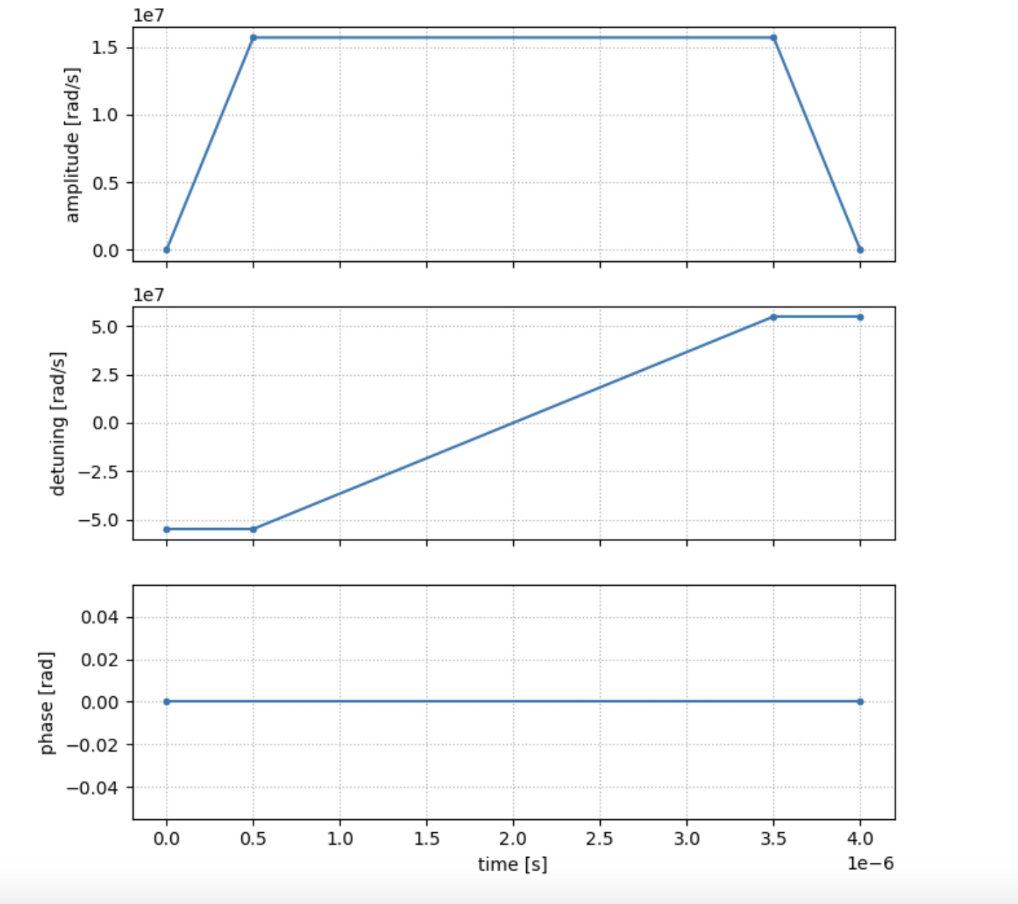
Analog calculations with arrays of Rydberg atoms have been performed with Aquila. We accessed Aquila using the AWS Braket services. We used the AWS Braket SDK for local simulations. This imposes constraints not present in exact diagonalization. In the following, we will focus on the single chain model with the same , and . The linear size of the system needs to be less than m. This means that we need . The distance between the atoms needs to be more than m which implies . We used the values . More importantly, the ground state needs to be prepared adiabatically and actual measurements are performed after turning off . The procedure suggested on the AWS Braket tutorials and also used in Zhang et al. (2024) lasts 4 and involves ramping down during the last 0.5 s, as illustrated in Fig. 4.
Appendix E Entropy errors
In this supplemental information section, we discuss errors for the local simulator with no ramping down (LSNRD), the local simulator with the standard ramping down (LSST) as in Fig. 4, and the actual device Aquila. We started with the local simulator and found some dependence on the details of the ramping down of at the end. The local simulator allows us to try time sequences not possible with the actual device. In order to check that the adiabatic preparation is working well, we started with flat at the end (so MHz after 4 sec instead of ramping down to zero after 3.5 s as in Fig. 4). We used 1000 shots and repeated the experiment ten times in order to estimate the statistical errors. The results are shown in Fig. 5 and show good agreement with exact diagonalization. Except for 1.1, 1.2 and 2.0, the values obtained with the local simulator agree with less than one standard deviation with the exact diagonalization results. This gives us confidence in the adiabatic preparation of the ground state.
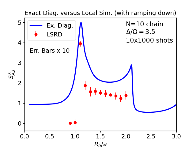
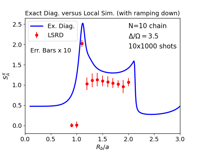
We repeated the local simulation with the realistic ramping down at the end shown in Fig. 4. The results are shown in Fig. 6. The agreement is not as good as in Fig. 5. The size of the statistical errors bars are much smaller than the discrepancies with exact diagonalization for and . However the error somehow cancel in and we obtain reasonable estimates of .
We repeated parts of these simulations with the actual device and we can now compare the estimations of and obtained with: 1) exact diagonalization, 2) the local simulator with no ramping down (LSNRD) as in Fig. 5, 3) the local simulator with the standard ramping down (LSST) as in Fig. 6, and 4) the actual device Aquila. We focus the discussion on . In cases 2), 3) and 4) we used two independent runs with 1000 shots. By dividing the number of events by 1000, we obtain estimations of the probabilities that can be calculated exactly.
The results involving more than 10 counts are shown in Table 1 and lead to the conclusions that:
-
•
LSNRD provides reasonably accurate estimations of the probabilities for states in the computational basis, for a broad range of values for the probabilities. This is not a surprise, it just shows that the local simulator works properly.
-
•
LSST removes states with low probabilities and significantly amplifies some medium probabilities such as 0.138 for rggrgrgrgr and rgrgrgrggr. This suggests that a more rapid ramping down maybe preferable for entropy estimation.
-
•
Aquila amplifies some of the low probability states and depletes higher probability states while keeping some ratios roughly in line with exact results.
From the above discussion, it is clear that there are significant fluctuations for states that are expected to be seen 10 times or less in 1000 shots. LSST removes these states while Aquila amplifies them. This suggests to discard results with low counts and proceed with truncated data sets. In the following we considered truncated data sets where states with 10 or less measurements were discarded. By doing this, the number of shots is reduced which leads to different probability estimates. The results of this truncation for the entropies are shown in Table 2. From these results we conclude that
-
•
The truncation lowers the entropies calculated with exact diagonalization by about 20 percent but increases by about 10 percent.
-
•
LSNRD follows closely the exact results. Again this was expected.
-
•
LSST is insensitive to the truncation. The LSST values are close to exact truncated values. Again this was expected.
-
•
Aquila results are very sensitive to truncation which brings the results closer to exact ones, but maybe not as close as hoped.
More generally, the truncation method seems to introduce significant uncertainties and we believe that error cancellations with the untruncated procedure may be more reliable.
| Entropy | Exact | LSNRD1 | LSNRD2 | LSST1 | LSST2 | Aquila1 | Aquila2 |
|---|---|---|---|---|---|---|---|
| grgrgrgrgr | 12 | 14 | 19 | 24 | 18 | 16 | 18 |
| rggggrgrgr | 16 | 21 | 18 | 15 | 14 | ||
| rggrgrgrgr | 138 | 142 | 152 | 201 | 222 | 136 | 149 |
| rgrggggrgr | 23 | 18 | 28 | 19 | 24 | ||
| rgrggrgrgg | 11 | 14 | (5) | ||||
| rgrggrgrgr | 276 | 232 | 239 | 274 | 264 | 174 | 175 |
| rgrgrggggr | 16 | 14 | 18 | 19 | 12 | ||
| rgrgrggrgr | 276 | 248 | 244 | 278 | 266 | 190 | 180 |
| rgrgrgrggr | 138 | 179 | 168 | 207 | 200 | 151 | 179 |
| rgrgrgrgrg | 12 | 13 | 18 | 12 | 25 | 23 | 16 |
| Total | 907 | 892 | 904 | 996 | 995 | 804(*) | 812(**) |
| Entropy | Exact | LSNRD1 | LSNRD2 | LSST1 | LSST2 | Aquila1 | Aquila2 |
|---|---|---|---|---|---|---|---|
| 2.126 | 2.241 | 2.198 | 1.527 | 1.558 | 2.944 | 2.874 | |
| 1.6476 | 1.734 | 1.740 | 1.504 | 1.527 | 2.035 | 1.901 | |
| 1.337 | 1.374 | 1.354 | 1.117 | 1.134 | 1.685 | 1.681 | |
| 1.131 | 1.149 | 1.167 | 1.115 | 1.108 | 1.288 | 1.233 | |
| 0.686 | 0.634 | 0.639 | 0.883 | 0.888 | 0.531 | 0.611 | |
| 0.769 | 0.706 | 0.742 | 0.907 | 0.861 | 0.676 | 0.707 |
Appendix F Second-order Rényi entropies