Beable-guided measurement theory
Abstract
Measurement model in the de Broglie-Bohm theory is developed. Following von Neumann principles, both the measurement device and the target system are described by the same quantum laws. This investigation includes basic models of coordinates and momentum measurements. Equations for pilot waves are solved analytically, and de Broglie particles trajectories are calculated numerically. The resulting model resolves the issues related to probability distribution in momentum space that were addressed in the works [Kurt Jung 2013 J. Phys.: Conf. Ser. 442 012060], [M. Nauenberg 2014 Quanta 3, 43], [D. M. Heim 2022 arXiv:2201.05971v1]. Origin of quantum contextuality in the de Broglie-Bohm theory is discussed. Further, a new problem is considered: whether the de Broglie-Bohm theory admits Heisenberg uncertainty principle in special thought experiment, where momentum and coordinate are measured in turns several times. By direct calculation, we show that uncertainty relation is restored due to turbulence-like perturbations. We consider also the measurement models which do not admit this mechanism and thus may open up new possibilities for experimental testing of the de Broglie-Bohm theory.
pacs:
03.65.Ta Foundations of quantum mechanics; measurement theoryI Introduction
The measurement problem neumann ; bohr_1 ; bohr_2 ; Frauchiger ; collapse ; men ; bar can be formulated as a question of understanding why a single macroscopic result emerges from a measurement process, while solutions of quantum mechanics equations indicate that several results occur simultaneously oxford_handbook . Due to von Neumann insolubility argument mathematical apparatus of quantum mechanics is not enough to resolve this problem111The relation between decoherence and quantum measurement have been extensively discussed in the literature dec_max_1 ; dec_max_2 ; dec_zeh ; dec_zurek . The dedicated discussion is present in our work neumann . That is why an additional assumption is needed to solve the measurement problem. Several interpretations of quantum mechanics provide the assumption. In this sense, they are an expansion of quantum mechanics. But the next problem is to choose between these interpretations, since all of them usually have the same experimental predictions (that is why interpretations are often considered as purely philosophical issues). Thus, it is specially interesting to find cases when some interpretations provide new predictions or, on the contrary, have problems with self-consistency and reproducing quantum mechanic basics. Such interpretations can be considered not just as interpretations but as full-fledged falsifiable theories.
This paper is devoted to the description of measurement process in the de Broglie-Bohm theory. The de Broglie-Bohm theory is deterministic interpretation of quantum mechanics with non-local beable parameters epr ; bell_1 ; bell_2 that was originally proposed by Louis de Broglie in the 1920s deB and rediscovered by David Bohm in 1952 bohm_1 ; bohm_2 . Subsequently, numerous efforts have been made to advance and refine this theory. Significant progress is made on deterministic quantum field theory bohm_3 ; str_1 ; str_2 ; nic_1 ; nic_2 . Some discussions have revolved around the process of restoring quantum equilibrium val and there have even been proposals to explain phenomena like dark energy and dark matter within the de Broglie-Bohm framework kent . Weak measurements aaronov_1 ; aaronov_2 were carried out, in which the Bohm trajectories for single photon were restored after diffraction on the double-slit interferometer Kocsis . The difference between these trajectories and those numerically modeled for non-relativistic particles Philip is discussed Flack_1 ; Flack_2 .
Some problems of the de Broglie-Bohm theory were discussed in the last time. Recent works by various authors kurt ; naun ; heim have raised concerns about a potential inconsistency between the predictions of the de Broglie-Bohm theory and the "usual" quantum mechanics. Specifically, when assuming a direct connection between a particle’s de Broglie velocity and its momentum, the theory appears to yield an inaccurate probability distribution in the momentum representation. It turns out, that explicit measurement process simulation resolves this problem, as it will be shown by direct calculation.
To describe the measurement we rely on von Neumann theory neumann . We will limit ourselves to projective measurements (also called non-destructive or strong brag_1 ; brag_2 ; brag_3 ; vor ). Namely, we will consider the projective measurements of momentum and coordinates of a free particle.
Another problem under consideration is a possible violation of the Heisenberg uncertainty principle hies in the de Broglie-Bohm theory at the non-destructive measurements of coordinate and momentum. The uncertainty relation is a direct consequence of the quantum mechanics postulates and remains valid, including for non-destructive measurements: by any measurement of a quantity, information about the observed quantum conjugate is lost. However, in a deterministic interpretation, it can be assumed that some of the information is stored in de Broglie particles (particles’ de Broglie velocities). For example, we can propose an experiment in which the coordinate is measured first, then the momentum and then the coordinate again. Due to the deterministic nature of the theory, the result of the second coordinate measurement depends on the position of the de Broglie particle after the first measurement that potentially can violate the uncertainty relation. The violation will not take place if and only if the momentum measurement introduces sufficient disturbances to the coordinate of the system.
The paper is organized as follows. The Sec. II devotes to description of measurement process in the de Broglie-Bohm theory using von Neumann measurement theory. In the Sec. III and IV the simplest coordinate and momentum measurement devices are developed. The de Broglie particles behaviour in the measurement processes is analyzed. In the Sec. V relationship between decoherence process and measurement is considered. The measurement time is estimated. In the Sec. VI momentum probability distribution is restored and thus problem posed in the recent works kurt ; naun ; heim is solved. Sec. VII is devoted to quantum contextuality in the de Broglie-Bohm theory and device influence on measurement result. In the Sec. VIII thought experiment, in which violation of Heisenberg principle may occur, is considered. It is shown, that stochastic fluctuations during momentum measurement restore uncertainly principle. In the Sec. IX we discuss our results and prospects of the direction.
All calculations are made in units.
II Description of measurement process
in the de Broglie-Bohm theory
The wave function in the de Broglie theory is the physical field and it is called a pilot-wave. It obeys the Schrdinger equation
| (1) |
dynamics of particles is determined by guidance equation
| (2) |
here is probability current density, is probability density. Thus particle dynamics is deterministic one opposite to "Copenhagen paradigm".
If corresponds to the probability density of the particle distribution at some point in time, then this equality stays in the future. This state of the particles ensemble is called quantum equilibrium deB ; bohm_1 ; bohm_2 . The conservation of the quantum equilibrium provides correspondence to the quantum mechanical predictions. In the work val it is shown that an arbitrary system in the evolution process tends to a quantum equilibrium state in a finite time. Thus, the de Broglie theory reproduces predictions of quantum mechanics without assumptions about the probabilistic nature of the measurement process. In this paper, it is assumed that the system is initially in quantum equilibrium.
We use Bohm’s quantum measurement theory bohm_2 and von Neumann theory neumann for modeling measurement devices. In the von Neumann theory the device has one degree of freedom. It is a strong simplification because a real measurement device has a huge number of degrees of freedom, but it is sufficient to describe all key features of the real device. According to the Bohm theory, the device, as well as the measured system, has de Broglie coordinates. These coordinates can be considered as the device needles. The measurement process is an entanglement of the wave functions of the device and the quantum system
| (3) |
Here is the evolution operator, is initial device wave-function, and are eigenfunctions of the observable operator, and are amplitudes, and are wave-functions of the device in the states, when it measured corresponding values. The simplest case is schematically presented here, when a quantum system is initially in a superposition of two eigen-states.
The corresponding trajectories of the de Broglie particles are intertwined. The quantum system wave-function and the device wave-function guide target system de Broglie particles and device particles (device needles) accordingly. Moreover, due to entanglement of wave functions the device needles and quantum system particles turn out to be correlated and thus their trajectories are intertwined. Thus the measurement result is encoded in the device particles coordinates str_2 . The ensemble of such trajectories provides an opportunity to observe what actually happens to the quantum system and the device during the measurement process and thus separate the influence of the device on the system and the system on the device. Such an opportunity is provided by the de Broglie interpretation of the measurement process.
A simple model of the evolution operator can be constructed by introducing the Hamiltonian of the interaction between the device and the quantum system. In accordance with von Neumann’s measurement theory, interaction Hamiltonian must commute with the operator of the measuring value , and depend on the momentum of the device needle so that the needle coordinate encodes the measurement result
| (4) |
where is a needle coordinate. The simplest form of such Hamiltonian is
| (5) |
here is coupling constant.
Evolution due to this Hamiltonian makes the needle move in different ways depending on the observable values.
In the case of projective measurement solution of the Schrdinger equation with the Hamiltonian is
| (6) |
here is the device wave-function corresponding to the physical value and is eigenfunction of the .
In order to clarify the essence of the approach and not complicate the work with cumbersome calculations we will restrict ourselves to the simplest one-dimensional model. The point device has a coordinate and momentum , and the target quantum system consists of a single particle with a coordinate and momentum . At the same time, the device is considered massive enough to model its classicity and thus to minimize the disturbances introduced by the quantum system. The wave function of the device is chosen to be real in order to take into account only quantum disturbances introduced by the device.
III Coordinate measurement
Now let us construct a description of the coordinate measurement. According to the Sec. II, the simplest device-system interaction Hamiltonian has the form
| (7) |
where is the particle coordinate, is the device needle coordinate, is the coupling constant. Thus Schrdinger equation is
| (8) |
the components of the current will be
| (9) |
and guidance equations take the form
| (10) | |||
| (11) |
We can see from the guidance equations, that the device velocity depends on the position of the quantum system, that is why it is the coordinate measurement.
We consider the measurement process in the limit, when it can be described as projective one. The measurement should take place in a sufficiently short time so that the mobility of the quantum system associated with the kinetic term does not significantly affect on the measurement result. The analogues effect can be achieved by increasing the intensity of interaction between the quantum system and the device (increasing the coupling constant ). In both cases kinetic contribution can be neglected (see more detailed discussion in Sec. V). In this approximation the reduced evolution equation takes the form (compare with the general equation (3))
| (12) |
The solution of (12) is an entangled state of the device and the quantum system
| (13) |
here is wave function of the quantum system in the coordinate representation, is eigenfunction of the coordinate operator, is wave function of the device in the coordinate representation at the initial point of time . The current density components are . The corresponding guidance equation for device keeps previous form
| (14) |
Thus coordinate measurement process in the projective measurement limit can be constructed in accordance with the von Neumann theory presented in the Sec. II.
IV The momentum measurement
To describe the momentum measurement, we use the simplest Hamiltonian of interaction with a device measuring momentum
| (15) |
where is the particle coordinate, is the device needle coordinate, is the coupling constant.
Schrdinger equation
| (16) |
Its solution is an entangled state of device and quantum system
| (17) |
here is wave function of the quantum system in the momentum representation, is eignfunction of the momentum operator, is wave function of the device in the momentum representation at the initial moment of time .
Current components will be
| (18) | |||
| (19) |
The corresponding guidance equations are
| (20) | |||
| (21) |
Let us consider the simplest case when the initial state of the system describes the particle with a certain momentum
| (22) |
The velocities of the device and target system particles are
| (23) |
The velocity of the needle corresponds to the particle momentum. It is momentum measurement in this case.
Now let us consider the superposition of momentums
| (24) |
In this case
| (25) |
where
| (26) |
The guidance equation for the target system and for the device will be
| (27) | |||
| (28) |
| (29) |
We will call phase difference as correlation phase, since it is the phase of the non-diagonal components of the density matrix (see Sec. V). At the end of the measurement process the product vanishes, and the velocity of the device and the measured particle take the values one of the and values, accordingly.
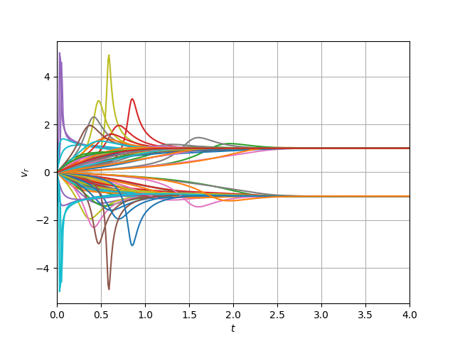
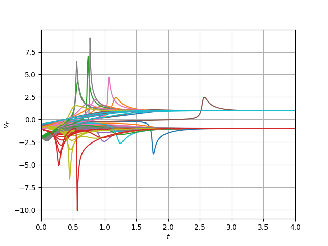
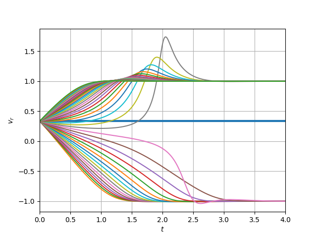
To describe the measurement process in details let us consider the results of numerical solution of guidance equations for the case of a superposition of two momentums. On the Fig. 1 the dependencies of the device needle velocity on time are shown under various initial conditions. The initial device wave-function is taken in the Gaussian form . The initial distribution for the device and the target system beables are selected in accordance with the Born rule.
It can be seen on Fig. 1, that the device trajectories are intertwined with the measured quantum system trajectories. During the measurement time , the system behaves itself chaotically, but then it enters one of the two stationary (classical) trajectories. The device needle acquires a velocity proportional to either or . Thus the momentum is measured indeed.
Strong fluctuations during the measurement are associated with the mutual influence of the device and the quantum system provided by quantum potential. The Heisenberg uncertainty relation is directly related to these perturbations, as will be shown below.
Note that for there are points of zero particle density. At these points, the guidance equations are bad defined, so significant resonant bursts are observed near these points at the initial moments of time. Since the contribution of these areas is small, they were excluded from consideration.
We also indicate on the dependence of the oscillation frequency on the difference in the measurement process. So Fig. 1c shows the result of the numerical simulation at , , and a reduced mass of the quantum system by 100 times. A significant increase in the frequency of disturbances is clearly visible compared to the Fig. 1b. Thus the less mass of quantum system the more quantum disturbances occur with it.
Thus, momentum measurement, as well as coordinate measurement, can be modeled in full correspondence with general theory described in Sec. II.
V Decoherence process and measurement time
Let us discuss the relationship between the decoherence phenomenon and the measurement process in the de Broglie-Bohm theory. The decoherence is the entanglement of the wave functions of the target system and the device, in which the density matrix of the target system is diagonalized men . Decoherence always take place during the measurement process. However, the measurement process is not limited to decoherence. Indeed, diagonalization of the density matrix by itself does not mean that only one of the values of the physical magnitude will be measured. In the de Broglie-Bohm theory, decoherence is responsible for the separation of wave packets corresponding to different measurement outcomes, while the dynamics of de Broglie particles is responsible for the "choice" between these outcomes. At the same time, as it will be shown below, the measurement time may or may not coincide with the decoherence time.
In general case, from Eq. (6) the density matrix of the quantum system has the form
| (30) |
here is the device wave-function corresponding to the physical value and is eigenfunction of the operator .
Non-diagonal elements of the density matrix are proportional to products . Thus decoherence time is time, during which this product vanishes due to space separation of device wave packages
| (31) |
To make numerical estimation we assume that the device wave-function has a Gaussian form before measurement
| (32) |
Since 99,7 % of data concentrate within standard deviations from the average value then condition (31) will be fulfilled almost exactly if the difference between Gaussian peaks is at least standard deviations
From where the decoherence time is estimated as
| (33) |
Therefore decoherence occurs faster in the strong coupling regime and for highly distinguishable values of the target system physical quantities.
Let us consider momentum and coordinate measurements in more detail and compare decoherence time with time of measurement.
In the case of momentum measurement decoherence and measurement times coincide. Indeed, density matrix takes the form
| (34) |
and in the case superposition of momentum (24)
| (35) |
Thus, is the decoherence condition. But from guidance equations (27) follows, that condition is also a measurement condition. For the examples on Fig. 1a and Fig. 1b the measurement time estimation is (). It can be seen that most trajectories reach the stationary before this time.
In the the case of the coordinate measurement decoherence and measurement times are different. Indeed, while matrix density becomes diagonal after decoherence time
| (36) |
from guidance equation (14) we can see that the device needle velocity is proportional to coordinate of the target system from the beginning. It provides potential opportunity of the coordinate measurement in the mixed state discussed in the Sec. VIII.
Thus, the measurement time of the coordinate may not coincide with the decoherence time. Moreover, it seems that the measurement time can be made infinitely small222The discussion of the related issue of fulfilling the uncertainty relation in the de Broglie theory see in the Sec. VIII of this paper. However, this result is due to the fact that a simplified measurement model is used. A more realistic model also includes an amplification stage, during which decoherence occurs with the classical part of the device vor . Therefore, we can expect that in such model, the measurement time will exceed the decoherence time, although the question seems open.
It is necessary to estimate the characteristic measurement time for which the solution in the form of an entangled state (13) is suitable, i.e. to find the condition of projective measurement. For this we are to find conditions when kinetic term can be excluded. Substituting (13) into kinetic term in the equation (8) we obtain the condition
| (37) |
And we see that the solution (13) is useful while target system mass is large and while characteristic measurement time satisfies the following condition
| (38) |
It follows that coordinate measurement has to be realized in the weak coupling mode (the coupling constant has to be small) to be projective. The result is explained by quadratic increase of the kinetic term with an increase in the coupling constant compared to the linear increase of the term responsible for the interaction.
And thus coordinate measurement in more realistic device model should be carried out in a time satisfying the two opposite ratios (33) and (38). These conditions are corrected in the sector of the large coordinate differences.
In order to understand the reason for difference between measurement time in coordinate and momentum measurements, consider the role of the quantum potential. Stochastic perturbations in the coherent state are directly connected with the quantum potential. After measurement process, the quantum potential disappears and we observe the measurement result. That is why, if there is a quantum potential, measurement time is decoherence time. But in the absence of the quantum potential action, the measurement time has no lower bound while decoherence time is finite. In Sec.VII it will be shown actually that in the coordinate measurement there is no quantum potential.
Thus the de Broglie-Bohm theory demonstrates that decoherence phenomenon does not provide solution of the measurement problem because decoherence phenomenon does not explain selectivity of the device in the measurement process. In the de Broglie-Bohm theory we have this explanation by deterministic behaviour of the de Broglie particles.
VI Born’s rule for the momentum probability distribution
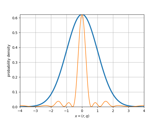
If we associate the velocity of a de Broglie particle with its momentum , as it was done in kurt ; naun ; heim , then an incorrect probability distribution in the momentum representation will arise. However, now we show that explicit simulation of the measurement process provides correct momentum distribution.
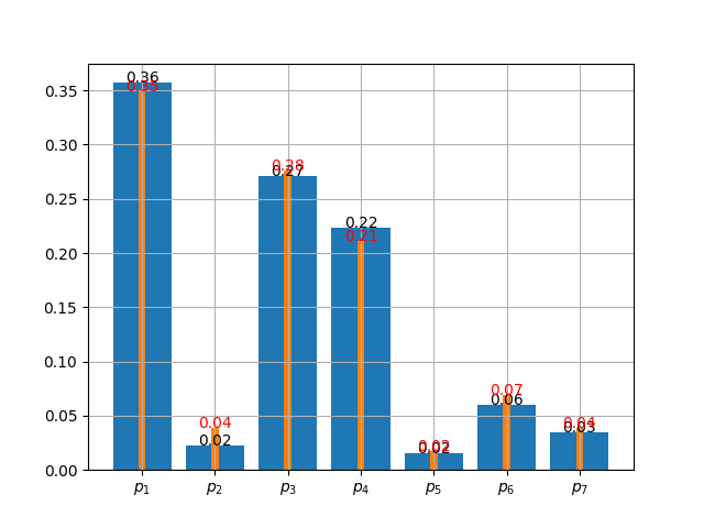
Having distributed the de Broglie device particles in accordance with Born’s rule at the initial moment of time, we numerically find the distribution of the device particles by velocities after measurement. In Fig. 2 it is clearly seen that this distribution reproduces the distribution in the target system that was in a superposition state with momentums at a random probability amplitude. Thus, explicit modeling of the momentum measurement process solves the problem with the probability distribution in the momentum space posed in kurt ; naun ; heim .
To solve the problem, we refuse on the direct connection between the measured momentum and the de Broglie velocity. It means that the de Broglie velocity of the particle is not a quantity directly measured experimentally – it is a hidden parameter. Moreover, direct connection between the observable and the hidden parameter contradicts quantum contextuality (see Sec. VII). The principle states that the measurements of quantum observables cannot simply be considered of as revealing preexisting values. The de Broglie velocity is such a preexisting value and it can only be measured after decoherence process.
VII The influence of device on measurement results
It is a well-known statement that in quantum mechanics all physical quantities are contextual bohr_2 ; bric . It means that quantum system is not described by a specific physical quantity outside the context of its measurement (see also Sec. VI). According to Bohr it indicates on the active role of the device in quantum mechanics, as opposed to the device passive role in classical mechanics bohr_2 . That is why, investigation of the contextuality in the theory with hidden variables is of particular interest.
In the de Broglie-Bohm theory, the active influence of the device on the measurement result is associated with the dependence of the measurement result on the initial states of the device particles bric . Thus, different values of the same physical quantity can be measured for the same quantum system with fixed de Broglie coordinates, depending on the initial conditions for the device needles.
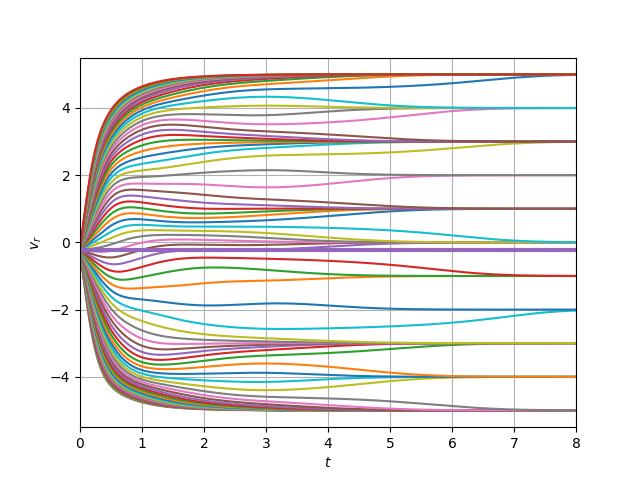
The device influence on measurement result can be observed in the momentum measurement process. To demonstrate this on Fig. 3, we fix the initial condition for the target system and observe that the measurement result does depend on the initial position of the device needle.
However in the case of the coordinate measurement in the simplest model developed in Sec. III such contextuality is not observed since de Broglie velocity directly connected with coordinate of the target system. Thus, at least in the case of the simple model, the coordinate of the target system particle defines the measurement result. This fact is strongly is connected with the infinitely small measurement time for this case, discussed in Sec. V.
The quantum contextuality in the de Broglie-Bohm theory is directly connected with the presence of the quantum potential. Namely, the action of the quantum potential provides contextuality.
In the case of the momentum measurement after substitution taking into account the reality of the wave function of the device in the equations (20), (16) we get guidance equations in the form
| (39) | |||
| (40) |
and quantum Hamilton-Jacobi equation for :
| (41) |
where the last pair of terms is the quantum potential. The presence of non-local contributions of the quantum potential induces the non-local interaction of the device and the target system. If the quantum potential is zero so would be a classical action, and from (40) it follows that beable velocity is connected to canonical momentum. Indeed, in the classical limit the quantum potential vanishes, and the de Broglie velocity is directly associated with measured momentum as shown in Fig. 3 (bold line). But in general case due to non-locality of the quantum potential the de Broglie particle velocity turns out to be associated with not one but all potentially observable momentums. Therefore, there is no direct connection between the measured momentum and the velocity of the de Broglie particle.
It should be noted that the interaction between device and target system has purely quantum nature due to equation (40) describes free non-relativistic particle in absence of quantum potential. The feature is connected with assumption of device wave function reality.
In the case of coordinate measurement the quantum potential is absent in quantum Hamilton-Jacoby equation regardless of the reality or complexity of the device wave function:
| (42) |
That is why no contextuality observed in the considered coordinate measurement model. Note that in the interaction model
| (43) |
quantum potential is presented where . Nevertheless, investigation of it is not necessary within the framework of the tasks set.
Thus, in the de Broglie-Bohm theory the measurement result depends on the both initial position of the target system and the device beables. This feature admits the principle of quantum contextuality. However in the simple coordinate measurement model the device beable position does not affect the measurement outcome, which breaks the contextuality: observable quantities can be considered objectively describing a quantum system.
VIII The uncertainty principle
Although de Broglie’s theory is deterministic in its content, it is expected that the uncertainty relation will be fulfilled causing the stochastic behavior of systems. Let us consider the following thought experiment in which this relationship may be violated. At first we measure the coordinate of the particle, then its momentum, and then the coordinate again. After the first coordinate measurement the wave packet is localized. After momentum measuring, the wave packet spreads (which causes the uncertainty ratio in quantum mechanics). However, the de Broglie particle may retain information about the position of the particle at the localization moment. In order to the uncertainty relation to be fulfilled, it is necessary the sufficiently strong unpredictable changes are made to the de Broglie particle coordinate during the momentum measurement. Otherwise, when re-measuring the coordinate (after the momentum measuring) we can predict the measurement result with greater accuracy than the axioms of quantum mechanics allow.
We use devices that are described in the previous sections for the experiment. The Schrdinger equation for this process
| (44) |
here
| (45) | |||
| (46) |
are measurement time that are determined by (33) and (38) accordingly.
After the first coordinate measurement, the wave-function will be delta-function according to (13). The following momentum measurement will start with this delta-function. Thus, in expression (17) we find by making Fourier transform:
| (47) |
To make a numerical calculation, we consider the regularized delta-function and its approximate Fourier transform, valid in the finite space region:
| (48) |
The regularized delta-function for is shown in Fig. 4. As will be shown, these values are sufficient to restore the uncertainty ratio for any parameters of the task.
As was mentioned above, momentum measurement plays a crucial role here by inducing certain perturbations into the coordinate. In order to estimate these perturbations, we consider all possible trajectories of particles starting in a localized region and finishing with the measurement of the same momentum, but corresponding to different initial positions of the device. We consider the trajectories reaching a given stationary velocity since this velocity is equal to the observed momentum by the end of the measurement process. Note that the dispersion of the coordinates of such a group of particles is significantly small than the dispersion of all particles.
Since expression (48) is approximate one, it would lead to zero momentum uncertainty after the momentum measurement. But after the more realistic measurement some residual momentum uncertainty remains. To estimate this uncertainty we notice that in order to resolve closer momenta, more time is needed (see expression (33)). In accordance with it the measurement time in the case under consideration corresponds to the resolution time of all momentums differing by more than . Therefore, to check the fulfillment of the uncertainty relation, we will consider the value of as the uncertainty of the momentum after passing the measurement time.
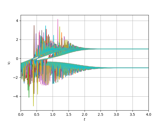
In Fig. 5 the result of the numerical solution of the guidance equation (27) is presented in the case of states with certain moments, with values from to in conventional units. Fig. 6 shows the dependence of the product ( is the coordinate dispersion) on time. It can be seen from the figure that the stochastic perturbations arising in the measurement process are sufficient to fulfill the uncertainty relation.
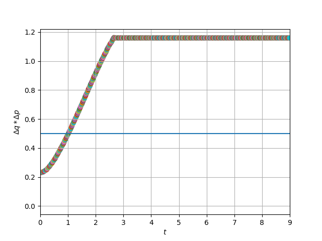
With the increase of the number of values in a fixed range, the inaccuracy of the momentum measurement decreases. This provides an increase in the resolution time of this difference according to the equation (33). It means an increase of stochastic oscillations in the time and it provides an increase in the coordinate dispersion of the quantum system . Thus, a further increase in the accuracy of the momentum measuring and the range of possible values (increased localization of particles of the quantum system) provides a corresponding increase in the coordinate dispersion and provides the fulfillment of the uncertainty principle.
So, there is a mechanism for restoring the uncertainty ratio: stochastic perturbations of the de Broglie particles coordinates introduced by the momentum measured device.
However, the situation is not so clean in another thought experiment: at first momentum measurement, than the coordinate and the momentum once more. As it was shown in Sec. V the simple model admits an instantaneous coordinate measurement, which induces no disturbances in the target system. Thus, we have a violation of the Heisenberg principle using the coordinate measurement model, described in Sec. III. To investigate weather the uncertainty relation restored in all situations, we need to consider the more realistic measurement model, as discussed in Sec. V.
But detailed consideration of it is beyond the scope of our consideration.
IX Discussions and conclusions
We proposed the procedure for the quantum non-destructive measurement of the coordinate and the momentum in the de Broglie-Bohm theory.
The correct momentum probability distribution predicted by the quantum theory apparatus has been restored. Thus, the problems that have been formulated by several scientific groups kurt ; naun ; heim were discussed and the solution to these was proposed.
The mechanism of the quantum contextuality emergence in the de Broglie-Bohm theory is established, namely the presence of a non-local quantum potential provides dependence of the target system state on the state of the device during the measurement. It might seem that the dependence of the measurement result on the device state gives the observer the ability to control the measurement outcome. However, it is not obvious whether it is possible to manage the initial state of the device with such accuracy. Furthermore, in the more detailed measurement model, the state of the target system entangles not only with the device state, but also with the environment, which increases stochasticity. Thus, the measurement result cannot be completely determined by the initial state of the system under study and is random.
In the investigation, the fact that the measurement process is not reduced to decoherence has significantly manifested itself, although it plays a key role. In particular, the decoherence time may not coincide with the measurement time.
It turned out that the coordinate and momentum measurement models which can be understand very similar and built from the same considerations have fundamental differences. In the case of the coordinate measurement, the quantum potential can be neglected if the measurement is carried out quickly enough. In the case of the momentum measurement the quantum potential is irreplaceable. While in other interpretations such a difference may be uncritical but in the de Broglie-Bohm theory it is fundamental. The momentum measurement model has many important qualities, namely contextuality, coincidence of decoherence time and measurement time. On the contrary, the proposed coordinate measurement model does not have such properties. The measurement time in this model can be made arbitrarily small, which leads to the contextuality violation. Apparently, the presence of such non-contextual measurement models is a characteristic feature of the de Broglie-Bohm theory.
A thought experiment is proposed and modeled, in which a violation of the Heisenberg uncertainty relation can potentially occur - an alternate measurement of the coordinate and the momentum. The numerical modeling has clearly shown that the measurement of the momentum leads to strong stochastic fluctuations in the coordinate of the quantum system, which is a mechanism for restoring the uncertainty ratio. However, due to the lack of quantum potential, the coordinate measurement model does not provide a similar mechanism. It leads to a violation of the uncertainty ratio if the momentum is measured in the first place and then the coordinates and again the momentum.
Thus, the de Broglie’s theory shows full agreement with the axioms of quantum mechanics, in particular with the Born rule. However, within the framework of the coordinate measurement there are problems with restoring contextuality and the ratio of uncertainties. Apparently, these problems are related to the fact that the coordinate measurement model is too simple. This issue requires further research. Perhaps this opens up new prospects for experimental verification of the de Broglie-Bohm theory.
To better understand the results, the pilot-wave can be thought of as a quantum liquid. The de Broglie particles are point detectors moving along the current lines of this liquid. The demonstrated stochastic perturbations can be interpreted as a certain turbulent process occurring with a quantum fluid in the measurement process – mixing of the quantum fluids of the device and the target system, respectively. In this case, the de Broglie particles are test granules placed in this liquid. The assumed irreversibility and contextuality in the measurement process is associated with precisely these fluctuations. A similar situation was described by Bohm in work bohm_1 . In this paper, Bohm pointed out the complicated nature of the de Broglie particles trajectories during measurement, resembling Brownian motion.
At the classical level, all observed quantities are an averaged values according to the fluctuations of the quantum liquid (fluctuations of beable variables) and the classical behavior is effectively restored, as can be seen from Fig. 3. Therefore, at the classical level, there are no irreversible and contextual effects in the measurement process, and every observable (essentially averaging over beable variables) objectively describes the physical state. The observation of the apparent turbulent behavior of a quantum liquid turns out to be possible in the processes of interaction with highly inhomogeneous structures (inhomogeneity of the order of the given liquid wavelength), such as a crystal lattice. A simplified model of such an interaction during the measurement was considered in this paper.
The further development of this research may be made in two directions. The first is related to the search for new effects predicted by the de Broglie-Bohm theory. The second is the investegation of the mathematical structure of the theory and the identification of new mathematical techniques. The details of these investigations will be discussed in our further papers.
X Acknowledgements
We would like to thank Yuri P. Rybakov, Anatoly V. Borisov, Kirill A. Kazakov, Oleg G. Kharlanov, for useful discussions. We also acknowledge the support of the Department of theoretical Physics, MSU.
References
- (1) von Neumann, J., // Mathematical Foundations of Quantum Mechanics, Princeton University Press, Princeton, 1955.
- (2) Bassi A., Dorato M., Ulbricht M. // Collapse Models: a theoretical, experimental and philosophical review, Entropy 2023, 25, 645
- (3) Frauchiger D., Renner R. // Nature communications 2018, 9, 3711
- (4) Bohr N., Rosenfeld L. // On the question of measurability of electromagnetic field quantities, Kgl. Danske Vidensk. Selskab. Math.-Fys. Medd, 1933, 12(8), P. 1-65.
- (5) Bohr N. // Can Quantum-Mechanical Description of Physical Reality be Considered Complete?, Phys. Rev., 1935, 48. P. 696–702.
- (6) M.B. Menskii // Decoherence and the theory of continuous quantum measurements, UFN, 1997, 168, №9.
- (7) Barandes, J.A., Kagan, D. // Measurement and Quantum Dynamics in the Minimal Modal Interpretation of Quantum Theory, Found Phys., 2020, 50, 1189–1218.
- (8) O. Freire // The Oxford Handbook of the History of Quantum Interpretations, Oxford University Press, Oxford, 2022.
- (9) Schlosshauer M. // Decoherence and the Quantum-to-Classical Transition, Springer, 2007.
- (10) Schlosshauer M. // Decoherence, the measurement problem, and interpretations of quantum mechanics, Rev. Mod. Phys., 2004, 76, P. 1267.
- (11) Zeh H. D. // On the interpretation of measurement in quantum theory, Found. Phys., 1970, 1, P. 69-76.
- (12) Zurek W. H. // Environment-induced superselection rules, Phys. Rev. D, 1982, 26. P. 1826-1880.
- (13) Einstein A., Podolsky B., Rosen N. // Can Quantum-Mechanical Description of Physical Reality Be Considered Complete?, Phys. Rev., 1935, 47, P. 777–780.
- (14) Bell J.S. // On the Einstein-Podolsky-Rosen paradox, Physics, 1964, 1, P. 195–200.
- (15) Bell J.S. // On the Problem of Hidden Variables in Quantum Mechanics, Reviews of Modern Physics, 1966, 38, P. 447–452.
- (16) de Broglie L. // Electrons et Photons: Rapports et Discussions du Cinquime Conseil de Physique tenu Bruxelles du 24 au 29 Octobre 1927 sous les Auspices de l’Institut International de Physique Solvay, 1928, P. 105.
- (17) D. Bohm // A Suggested Interpretation of the Quantum Theory in Terms of "Hidden" Variables. I, Phys. Rev., 1952, 85, 166.
- (18) D. Bohm // A Suggested Interpretation of the Quantum Theory in Terms of "Hidden" Variables. II, Phys. Rev., 1952, 85, 180.
- (19) D. Bohm, Basil J. Hiley, P N Kaloyerou // An Ontological Basis for the Quantum Theory: II -A Causal Interpretation of Quantum Fields, Physics Reports., 1987, 144, 321.
- (20) W. Struyve // Pilot-wave theory and quantum fields, Rep. Prog. Phys., 2010, 73, 106001.
- (21) W. Struyve, H. Westman // A minimalist pilot-wave model for quantum electrodynamics, Proc. R. Soc. A., 2007, 463, 3115.
- (22) H. Nikolic // Bohmian particle trajectories in relativistic bosonic quantum field theory, Found.Phys.Lett., 2004, 17, P. 363.
- (23) H. Nikolic // Bohmian particle trajectories in relativistic fermionic quantum field theory, Found.Phys.Lett., 2005, 18, P. 123.
- (24) A. Valentini, H. Westman // Dynamical Origin of Quantum Probabilities, Proceedings of the Royal Society A: Mathematical, Physical and Engineering Sciences, 2005, 461, N. 2053, P. 253-272.
- (25) A. Kent // Beable-Guided Quantum Theories: Generalising Quantum Probability Laws, Phys. Rev. A. 2013. 87. 022105.
- (26) Aharonov Y., Albert D. Z., Vaidman L. // How the result of a measurement of a component of the spin of a spin-1/2 particle can turn out to be 100, Phys. Rev. Lett., 1988, 60, P. 1351.
- (27) Aharonov Y., Vaidman L. // Properties of a quantum system during the time interval between two measurements, Phys. Rev. A, 1990, 41, P. 11.
- (28) Kocsis S, Braverman B, Ravets S, et al // Observing the Average Trajectories of Single Photons in a Two-Slit Interferometer Science. 2011. 332. P. 1170.
- (29) Philippidis, C., Dewdney, D., and Hiley, B. J. // Quantum Interference and the Quantum Potential, Nuovo Cimento, 1979, 52B. P. 15-28.
- (30) Flack, R, Hiley, B. J. // Weak Measurements, the Energy-Momentum Tensor and the Bohm Approach, 20th Anniversary of the Novel Concept of Protective Measurements, 2014.
- (31) Flack, R., Hiley, B. // Weak Measurement and its Experimental Realisation, Journal of Physics: Conference Series. 2014. 504.
- (32) K. Jung // Is the de Broglie-Bohm interpretation of quantum mechanics really plausible?, J. Phys.: Conf. Ser. 2013. 442. 012060.
- (33) M. Nauenberg // Is Bohm’s Interpretation Consistent with Quantum Mechanics?, Quanta. 2014. 3. P. 43.
- (34) D. M. Heim // Revising de Broglie-Bohm trajectories’ momentum distribution, arXiv. 2022. 2201.05971.
- (35) C.M. Caves et al. // On the measurement of a weak classical force coupled to a quantum-mechanical oscillator. I. Issues of principle, Rev. Mod. Phys., 1980, 52, P. 341.
- (36) V.B. Braginsky, Yu.I. Vorontsov, K.S. Thorne // Quantum Nondemolition Measurements, Science, 1980, 209, P. 547 — 557.
- (37) V.B. Braginsky // Resolution in macroscopic measurements: achievements and prospects, UFN, 1988, 156, №1.
- (38) Yu.I. Vorontsov // Standard quantum limits of measurement error and methods of overcoming them, UFN, 1994, 164, №1.
- (39) Heisenberg, W., // The Physical Principles of the Quantum Theory, Dover Publications, 1930.
- (40) J. Bricmont // The De Broglie-Bohm theory is and is not a hidden variable theory, arXiv. 2023. 2307.05148.