A machine learning-based study of open-charm hadrons in proton-proton collisions at the Large Hadron Collider

Abstract

In proton-proton and heavy-ion collisions, the study of charm hadrons plays a pivotal role in understanding the QCD medium and provides an undisputed testing ground for the theory of strong interaction, as they are mostly produced in the early stages of collisions via hard partonic interactions. The lightest open-charm, $D^{0}$ meson ($c\bar{u}$), can originate from two separate sources. The prompt $D^{0}$ originates from direct charm production or decay of excited open charm states, and the nonprompt stems from the decay of beauty hadrons. In this paper, using different machine learning (ML) algorithms such as XGBoost, CatBoost, and Random Forest, an attempt has been made to segregate the prompt and nonprompt production modes of $D^{0}$ meson signal from its background. The ML models are trained using the invariant mass ($M_{\pi K}$) through its hadronic decay channel, i.e., $D^{0}\rightarrow\pi^{+}K^{-}$, pseudoproper time ($t_{z}$), pseudoproper decay length ($c\tau$), and distance of closest approach of $D^{0}$ meson, using PYTHIA8 simulated $pp$ collisions at $\sqrt{s}=13~{}\rm{TeV}$. The ML models used in this analysis are found to retain the pseudorapidity, transverse momentum, and collision energy dependence. In addition, we report the ratio of nonprompt to prompt $D^{0}$ yield, the self-normalized yield of prompt and nonprompt $D^{0}$ and explore the charmonium, $J/\psi$ to open-charm, $D^{0}$ yield ratio as a function of transverse momenta and normalized multiplicity. The observables studied in this manuscript are well predicted by all the ML models compared to the simulation.

I Introduction

To understand the fundamental nature of our Universe, accelerator facilities such as the Relativistic Heavy-Ion Collider (RHIC) and the Large Hadron Collider (LHC) perform proton-proton ($pp$) and heavy ion collisions at ultra-relativistic speeds. These collisions allow us to explore a unique state of thermalized and deconfined medium of quarks and gluons, known as the quark-gluon plasma (QGP). Understanding the QGP medium, which mimics conditions of the micro-second-old Universe, is crucial. Furthermore, it sheds light on the phase transition from the deconfined partonic phase to the color-neutral hadronic phase, where they are confined within the hadrons, thereby making a testing ground for QCD strong interaction dynamics. However, the QGP medium is extremely transient, having a lifetime of the order of $10^{-23}~{}\rm{s}$, before the quarks and gluons hadronize into a color neutral state. As a result, we can only detect the final state hadrons after the kinetic freeze-out. Therefore, precise probes are essential to investigate the characteristics of this deconfined partonic medium.

One such probe for the study of the deconfined phase is the heavy quarks (HQs), i.e., charm and beauty. The HQs are produced in the initial hard scattering. Their production time is characterized by $\Delta t>(\frac{1}{2m_{c,b}})$; $\sim 0.1~{}\rm{fm/c}$ for charm quarks and $\sim 0.01~{}\rm{fm/c}$ for beauty quarks, which is much shorter than the formation time ($\sim 0.3~{}\rm{fm/c}$) of the QGP medium [1, 2]. In addition, due to their masses being much larger than the temperature of the QGP medium, the probability of thermal production and annihilation of HQs is negligible. The HQs undergo Brownian motion in the thermalized medium of lighter quarks ($u,d,s$) and experience the entire evolution of the QGP medium. These HQs combine with the light-flavor quarks at the phase boundary or during the system evolution to form the open-heavy-flavor hadrons. The most abundant of them is the $D^{0}$ meson ($c\bar{u}$) due to its lowest mass among all the heavy-flavor hadrons. Furthermore, the $D^{0}$ meson originates from two sources following different topology. First, the prompt $D^{0}$ mesons, comprising of the charm quarks come directly from the initial hard scatterings and as the feeddown from the higher excited charm states ($D^{*}~{}(\rm{2007})^{0},D_{1}(\rm{2420})^{+}$). Second, the nonprompt production in which the charm quarks are produced through flavor-changing weak decays of beauty hadrons ($B^{0},B^{+}$) [3, 4]. It is essential to separate the prompt and nonprompt $D^{0}$ to understand the relative contribution from the charm and the beauty sector. This helps in studying the nuclear modification factor in charm and beauty sector separately, which may shed light on possible different mechanisms of energy loss in the QCD medium. Further, this helps in studying different phenomena like HQ transport and thermalization in the medium through anisotropic flow. In addition, the study of topological production of $D^{0}$ meson has several physics implications. Prompt $D^{0}$ meson can help to understand QCD medium and can provide a testing ground for the theory of strong interactions. Various observables are measured in experiments from the final-state hadrons to understand the interaction of the charm quarks in the QGP medium, where a comprehensible insight can be gained using prompt $D^{0}$ mesons as a probe. Since the nonprompt $D^{0}$ mesons are weak decay products of beauty hadrons, they are produced at a larger distance from the primary interaction vertex. Thus, using non-prompt $D^{0}$ mesons to understand initial partonic interactions may not be an ideal choice. However, the nonprompt production of the $D^{0}$ mesons can help to unveil the beauty production in both $pp$ and heavy-ion collision sectors.

Experimentally, the study of heavy-flavor hadrons acts as a test for the perturbative Quantum Chromodynamics (pQCD) calculations. Additionally, an indirect analysis of the beauty sector is done by estimating the production of nonprompt $D$ mesons [5]. Moreover, the azimuthal anisotropy in the momentum space of final-state hadrons is estimated, which acts as an observable to probe the QGP medium. The elliptic flow coefficient of $D$ meson is calculated in ALICE, STAR, and CMS experiments  [6, 7, 8, 9, 10]. Recently, the elliptic flow of the nonprompt $D^{0}$ meson has been estimated for $\rm{Pb-Pb}$ collision at CMS and ALICE  [11, 12] to understand the contributions coming from beauty hadrons. Additionally, the nuclear modification factor ($R_{\rm AA}$) is estimated to explore the energy loss by the HQs through interaction with the medium, taking $pp$ collisions as a baseline [13, 2, 14]. With the advancements of Run-3 detector upgrades and higher luminosity in ALICE, there is a significant opportunity for thorough and rigorous exploration of the charm and beauty sectors.

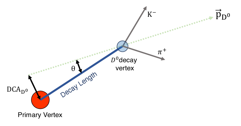
Figure 1: Schematic diagram of $D^{0}$ meson production and decay topology in hadronic and nuclear collisions.

Typically, $D^{0}$ meson is reconstructed through its hadronic decay channel $D^{0}\rightarrow\pi^{+}K^{-}$. The inclusive $D^{0}$ is dominated by prompt $D^{0}$ contributions, with only a small fraction is nonprompt $D^{0}$. Figure 1 provides a schematic diagram of $D^{0}$ production and $D^{0}\rightarrow\pi^{+}K^{-}$ decay topology. The decay length represents the distance between the $D^{0}$ decay vertex and the primary vertex. The distance of the closest approach of the $D^{0}$ meson (DCA${}_{D^{0}}$) is measured by taking the distance between the primary vertex and the reconstructed $D^{0}$ momentum vector $\vec{p}_{D^{0}}$. The beauty hadrons undergo a weak decay into a $D^{0}$ meson, which further decays into a $\pi^{+}K^{-}$ pair, whereas the prompt $D^{0}$ mesons are produced much closer to the primary vertex. The involvement of the weak interaction in the decay topology of the nonprompt $D^{0}$ meson increases the distance between the primary vertex and $D^{0}$ decay vertex. Consequently, the DCA${}_{D^{0}}$for the nonprompt $D^{0}$ mesons is higher than the prompt counterparts.

In this study, we take advantage of the machine learning (ML) techniques to separate the contribution from the charm and beauty sector by classifying the prompt and nonprompt $D^{0}$ mesons using final-state observables as input features. The ML algorithms, with proper training, are able to map a correlation between the input features and output. This is achieved through building a classification model from sample inputs, which allows the machine to learn independently and build a correlation between the inputs and outputs. Machine learning algorithms are categorized into supervised, unsupervised, semi-supervised, and reinforcement learning, each having its unique approach and application. In the case of experimental high-energy physics, the potential of machine learning lies in its ability to discover correlations in large datasets. ML techniques have been in use in the field of high-energy for the last few decades [15, 16, 17]. It is successfully deployed for studies like jet mesurements [18, 19, 20, 21], particle identification [22, 23, 24], impact parameter estimation [17, 25, 26], flow coefficient measurements [27, 28, 29]. Recently, classification problems, such as classifying prompt and nonprompt $J/\psi$ in forward rapidity [30] and segregating electrons coming from different sources [31] are addressed successfully. For our study of prompt and nonprompt classification of $D^{0}$, we simulate $pp$ collisions at $\sqrt{s}=13~{}\rm{TeV}$ using PYTHIA8 and train three different ML algorithms, namely XGBoost, CatBoost, and Random Forest. On successful training, we use our ML models to predict the production of prompt and nonprompt $D^{0}$ mesons for $pp$ collisions at $\sqrt{s}=5.02~{}\rm{TeV}$ and $900~{}\rm{GeV}$. The novelty of the work is reflected in the model’s robustness in distinguishing between prompt and nonprompt $D^{0}$ particles throughout the entire energy range of the LHC. On separating the prompt and nonprompt $D^{0}$ mesons, we attempt to understand their production dynamics with respect to the production of charged particles and charmonium state ($J/\psi$).

The remainder of the paper is organized as follows: in Section II, we briefly discuss the methodology of the work. Section III starts with a discussion of the training and evaluation of the models. Followed by the results and discussion in Section IV. Finally, we summarize and conclude our findings in Section V.

II Methodology

In this section, we present a brief introduction to event generation using PYTHIA8, followed by machine-learning algorithms. Additionally, the production cross-sections of prompt and nonprompt $D^{0}$ meson obtained from simulation are compared to published measurements from ALICE to quality check the tunes and settings used in PYTHIA8.

II.1 PYTHIA8

Event generators are used to simulate hadronic and heavy-ion collisions with greater control over the evolution stages and to test various phenomenological models. These generators use Monte Carlo simulation techniques to mimic the actual collisions involving a variety of physics processes. PYTHIA8, a Monte Carlo event generator, is commonly employed to simulate ultra-relativistic hadronic, leptonic, as well as heavy-ion collisions across a wide range of energy. It provides a comprehensive explanation of the pQCD-based particle production, including charm and beauty production. In this study, we use PYTHIA8 to simulate events for the training of machine learning algorithms to distinguish prompt and nonprompt particles.

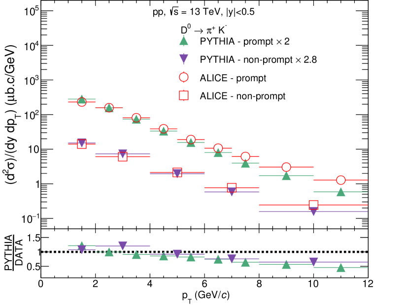
Figure 2: Upper panel shows the prompt and nonprompt $D^{0}$ meson production cross-section in $pp$ collisions at $\sqrt{s}=13~{}\rm{TeV}$ generated with PYTHIA8, compared with ALICE data [36, 38]. The lower panel depicts the PYTHIA8 to ALICE data ratio.

PYTHIA8 consists of particle production mechanisms involving soft and hard processes, initial and final state parton shower, string fragmentation, hadronic rescattering and decay, color reconnection, beam remnants, and multiple parton interactions (MPI). This is an improved version of PYTHIA6 that incorporates a scenario based on MPI. In this scenario, $2\rightarrow 2$ hard processes have the potential to generate heavy quarks such as charm and beauty. For this study, we have used PYTHIA 8.308, with 4C tune [34] ($\rm{tune:pp=5}$) and considering only inelastic and non-diffractive components ($\rm{HardQCD:all=on}$), to generate 2 billion minimum bias events for $pp$ collisions at $\sqrt{s}=13~{}\rm{TeV}$. Furthermore, we generate 1 billion minimum bias events for $pp$ collisions at $\sqrt{s}=5.02~{}\rm{TeV}$ and $900~{}\rm{GeV}$ each. To prevent the divergence of QCD processes, which can happen when transverse momentum, $p_{T}\rightarrow 0$, we implement a $p_{\rm T}$ cutoff of 0.5 GeV/c ($\rm{PhaseSpace:pTHatMinDiverge=0.5}$). The data have been simulated with color reconnection taken into consideration ($\rm{ColourReconnection:reconnect=on}$). Additionally, we have utilized the mode-2 for color reconnection, indicated by $\rm{ColourReconnection:mode=2}$. This mode refers to the gluon-move model, where the gluons are moved (or flipped) from one point to another such that the string length is minimized [33]. For the production of prompt and nonprompt $D^{0}$ mesons, we have enabled all the charmonium and bottomonium production processes via $\rm{Charmonium:all=on}$ and $\rm{Bottomonium:all=on}$. A detailed description of the physics processes and their implementation in PYTHIA8 are provided in Ref. [32, 33].

To mimic the real-world experiments, we enable the spread of the primary interaction vertex following a Gaussian distribution ($\rm{Beams:allowVertexSpread=on}$) as also done in Ref. [30]. The mean and sigma of the distribution in the cartesian coordinate are taken from Ref. [35]. Following the experimental methods, we have also taken a cutoff at the $z$ component of the interaction vertex, i.e., $|V_{z}|<10~{}\rm{cm}$. We have allowed the decay of $D^{0}$ through all the possible decay modes. In PYTHIA8, we examine the mother of the reconstructed $D^{0}$ meson to classify it into prompt or nonprompt $D^{0}$. In Fig. 2, we compare the PYTHIA8 generated $p_{\rm T}$ spectra with recent ALICE results [36, 38]. It is noteworthy that the CMS and LHCb experiments have measured only prompt $D^{0}$ in pp collisions, and their kinematic ranges are different [39, 40]. One can readily observe that the normalized yield of the prompt $D^{0}$ is around 10 times higher than the production of nonprompt $D^{0}$. The similar difference is continued up to the high-$p_{\rm T}$ range of around $12~{}\rm{GeV/c}$. PYTHIA8 underestimates the ALICE data, and hence, a factor of $2.0$ and $2.8$ is multiplied by the prompt and nonprompt yield, respectively to match the spectral shape. The trend of the $p_{\rm T}$ spectra shown by PYTHIA8, with all the above-mentioned tunes, is comparable with ALICE data as seen from the lower ratio plot. However, for the rest of the results, we do not apply any scaling factor to the PYTHIA8-generated spectra.

II.2 Machine Learning Algorithms

With the introduction of machine learning tools, drawing significant conclusions from a large set of experimental data has become easier and more reliable. This is achieved by properly taking care of the correlations among the input features. In experimental high-energy physics, one of the most complex problems is understanding the underlying physical processes in particle production in the subatomic realm. With the detected final state particles, one can use their four-momenta as input features to the machine learning algorithm. In this study, we use three machine-learning algorithms, namely, CatBoost (v1.2), Random Forest (v1.3.0), and XGBoost (v1.7.3). These ML techniques are very efficient for classification problems, each with its own unique strength. For instance, CatBoost is designed to handle categorical variables and does not require extensive data preprocessing like one-hot encoding. It also implements ordered boosting, a permutation-driven alternative to the classical algorithm, which improves the model prediction. On the other hand, Random Forest is an ensemble learning method that operates by constructing multiple decision trees during training and outputting the class that is the mode of classes of individual trees. It is highly flexible and efficient, even without hyper-parameter tuning. Lastly, XGBoost is a gradient-boosting framework that uses boosted decision trees. It implements parallel processing, which makes it fastest among all sequential gradient boosting techniques. It also includes parameter regularization to prevent overtraining, which is not available in most of the other algorithms.

These three models are often preferred over others due to their robustness, efficiency, and the fact that they can easily handle a variety of data types. They also have the ability to model complex nonlinear correlations, which adds to their versatility and utility in many real-world applications [37]. For training and prediction, we use Python 3.11 as well as computing and plotting the confusion matrix, importance score, and learning curve.

II.2.1 CatBoost

CatBoost stands for Categorical Boosting. It is a high-performance ML algorithm that has gained popularity due to its ability to handle categorical data directly, with no need for manual one-hot encoding [41, 42]. It’s an implementation of gradient boosting designed to combat the problem of overfitting by implementing a novel algorithm for calculating leaf values. CatBoost also supports GPU acceleration, which can significantly speed up the training process. It provides a wide range of hyper-parameters that can be fine-tuned to improve the model’s performance.

II.2.2 Random Forest

Random Forest is a versatile and widely used ML algorithm that operates by constructing multiple decision trees during training. It gives the output as the class, i.e., the mode of the classes for classification or mean prediction for regression tasks [43]. One of the key advantages of Random Forest is that it can be used for both regression and classification tasks. It provides a good indicator of the feature’s importance, handles high-dimensional spaces well, and can deal with unbalanced datasets. Random forest is also less likely to overfit than individual decision trees.

II.2.3 XGBoost

XGBoost (XGB), which stands for Extreme Gradient Boosting, is a highly regarded and extensively utilized ML algorithm [44, 45]. It is particularly effective in dealing with large datasets and excels in both classification and regression tasks. XGB is an advanced version of Gradient-Boosting Decision Trees (GBDT) and includes several improvements, such as parallel computing and tree pruning. These enhancements expedite the training process, enabling XGB to manage large datasets efficiently. Furthermore, XGB offers a broad range of hyperparameters that can be fine-tuned to enhance the performance of the model.

III Training and Evaluation

In this section, the topological features used as inputs for the ML models are defined, followed by data pre-processing and model training. Finally, a few quality assurance plots are presented to demonstrate the classification accuracy of the ML models.

III.1 Input to the machine

In this study, a few topological features are selected as the inputs to the ML models. Our goal is to utilize such features that can identify the topological production dynamics of prompt and nonprompt $D^{0}$ meson. First, the inclusive $D^{0}$ meson signal has to be identified over its background, followed by the identification of the prompt and nonprompt production modes. One can identify the inclusive $D^{0}$ meson signal from the background with the help of its invariant mass ($m_{\pi K}$), where a peak in the $m_{\pi K}$ distribution is observed around the $D^{0}$ mass. The identification of prompt and nonprompt $D^{0}$ can then be performed by looking at the variables sensitive to their decay topology. For example, as the prompt $D^{0}$ mesons are produced closer to the primary vertex as compared to the nonprompt case, this eventually leads to a larger decay length for the $D^{0}$ mesons coming from the decay of beauty hadrons. The topological variables associated with the displaced production vertex of the $D^{0}$ mesons are the pseudoproper time ($t_{z}$) [46], the pseudoproper decay length ($c\tau$) [47], and the angle ($\theta$) between the $D^{0}$ momentum vector and the vector joining the $D^{0}$ decay vertex to the primary vertex [48]. The pseudoproper time is defined as [46],

$$t_{z}=\frac{(z_{D^{0}}-z_{\rm PV})\times m_{D^{0}}}{p_{z}}$$ (1)

where $z_{D^{0}}$ and $z_{\rm PV}$ are the coordinates of the $D^{0}$ decay vertex and primary vertex along the beam direction ($z$-axis), $m_{D^{0}}\simeq 1865$ MeV is the mass of the $D^{0}$ meson taken from Particle Data Group [49], and $p_{z}$ is the momentum in the $z$-direction. The decay topology of the $D^{0}$ meson in the longitudinal direction is quantified by $t_{z}$, where $t_{z}$ is expected to have a higher value for the nonprompt $D^{0}$ mesons as compared to the prompt $D^{0}$ mesons that are produced closer to the primary vertex.

Similarly, one can also quantify the decay topology of the particles in the transverse plane using pseudoproper decay length ($c\tau$). One can write the pseudoproper decay length as [47],

$$c\tau=\frac{c~{}m_{D^{0}}\vec{L}.\vec{p_{T}}}{|p_{T}|^{2}}$$ (2)

where, $\vec{L}$ is a vector pointing from the primary vertex towards the $D^{0}$ decay vertex, i.e. $\vec{L}=\vec{V}-\vec{S}$. Here, $\vec{V}=(V_{x},V_{y},V_{z})$ is the position of primary vertex and $\vec{S}=(S_{x},S_{y},S_{z})$ is the position of $D^{0}$ meson decay vertex with respect to the global origin, i.e., ($0,0,0$). As already mentioned in Sec. II.1, we have used a Gaussian profile to randomize the position of the primary vertex in three dimensions to be consistent with experimental scenario. In experiments, we can reconstruct the $D^{0}$ decay vertex as the middle point on the distance of closest approach between the candidate pion and kaon trajectories. However, in PYTHIA8, this is not trivial, and therefore, we need to estimate the $D^{0}$ decay vertex ($\vec{S}$). One can calculate the same as using the following expression [30].

$$S_{i}=\frac{(t_{1}+d_{i,1}m_{1}/p_{i,1})-(t_{2}+d_{i,2}m_{2}/p_{i,2})}{m_{1}/p_{i,1}-m_{2}/p_{i,2}}$$ (3)

where $i=x,y,z$ is the spatial index, and $m_{1}$ and $m_{2}$ are the masses of the two decay products of the $D^{0}$ meson. $d_{i,1}$ and $d_{i,2}$ are the distances covered by the decay products in time $t_{1}$ and $t_{2}$ with momentum $p_{i,1}$ and $p_{i,2}$, respectively. Thus, using $\vec{V}$, and $\vec{S}$, one can obtain the value of $\vec{L}$ and consequently estimate the value of $c\tau$.

Finally, we use DCA${}_{D^{0}}$, which is well estimated in experiments, as another topological input variable to the machine-learning models. DCA${}_{D^{0}}$is defined in terms of the decay length and sine of the angle between $\vec{L}$ and the $D^{0}$ momentum vector $\vec{p}_{D^{0}}$ as [48],

$${\rm DCA}_{D^{0}}=|\vec{L}|\times\sin\theta.$$ (4)

As discussed earlier, due to the difference in the decay topology of prompt and nonprompt $D^{0}$ mesons, we can expect larger DCA${}_{D^{0}}$for the nonprompt $D^{0}$ meson. Thus, we proceed to train the machine-learning models with $m_{\pi K}$, and the above discussed topological variables such as $t_{z}$, $c\tau$ and DCA${}_{D^{0}}$ of the reconstructed $\pi^{+}K^{-}$ pairs as the input variables to the machine. The training is performed using 600 million minimum bias $pp$ collisions at $\sqrt{s}=13~{}\rm{TeV}$.

III.2 Pre-processing and training

The task of the ML models is to classify the prompt and nonprompt $D^{0}$ mesons from the background using the topological features of the reconstructed $\pi^{+}K^{-}$ pairs. However, the number of prompt $\pi^{+}K^{-}$ pairs is naturally smaller than the number of uncorrelated background pairs. Similarly, the $\pi^{+}K^{-}$ pairs coming from nonprompt $D^{0}$ meson is even smaller as compared to the prompt pairs owing to the smaller production cross-section of charm quarks from beauty decays than the direct charm production as shown in Fig. 2. Hence, an ML model trained with such a dataset shows a bias towards the most populated class, in our case, the background class. Hence, the trained model will show a higher degree of inaccuracy by frequently predicting the most populated class when applied to a testing set. This is known as the class imbalance problem. Thus, the pre-processing of the input dataset becomes essential to avoid this class imbalance problem, which also enhances the quality of the training data. This leads to an unbiased training that improves the classification accuracy of the ML models.

The class imbalance problem is often addressed via sampling techniques. We could use different sampling techniques to pre-process our training data, such as the oversampling or undersampling methods. Undersampling involves reducing the number of samples from the majority class to balance the number on instances from each class in the dataset. But this has a serious downside as it can discard potentially useful data during the process by reducing the training statistics. Oversampling, on the other hand, involves increasing the samples in the minority class. This is achieved by duplicating the samples in the minority class. However, creating duplicate copies of the data may sometimes lead to overfitting. In this study, we use the Synthetic Minority Over-sampling Technique (SMOTE) to create new samples for the minority classes [50]. SMOTE creates synthetic samples from the minority class instead of creating copies. By doing this, SMOTE provides better information to the model about the minority class. Before oversampling, the ratio background:prompt:nonprompt was 50:20:1, and the ratio changed to 15:5:1 after oversampling using SMOTE. Moreover, for training, testing, and validation purposes, we split our input data into 8:1:1 (train:test:validation) set.

With this pre-processed data and class imbalance challenge out of sight, we proceed to train the machine learning algorithms. The optimum hyperparameters related to the XGBoost, CatBoost, and Random Forest models are listed in Table 1, 2, and 3, respectively and are briefly discussed in the next paragraph.

XGBoost (XGB)
Parameter Value booster gbtree learning$\_$rate 0.3 n$\_$estimators 20 subsample 1 max$\_$depth 3 objective multi:softmax eval$\_$metric mlogloss

Table 1: XGBoost hyperparameters

CatBoost (CB)
Parameter Value learning$\_$rate 0.3 iterations 30 depth 5 loss$\_$function MultiClass eval$\_$metric MultiClass

Table 2: CatBoost hyperparameters

Random Forest (RF)
Parameter Value n$\_$estimators 30 max-depth 5

Table 3: Random Forest hyperparameters

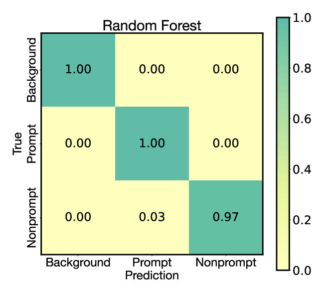
Figure 3: Confusion matrix for XGBoost (upper), CatBoost (middle), and Random Forest (lower), respectively. It represents the accuracy and discrepancy of the machine-learning models to predict the target classes.

In XGBoost, the booster decides the type of model that runs at each iteration. The gbtree booster uses tree-based models. The learning rate is a configurable hyperparameter that determines how much the weights in the model are adjusted during training. A higher learning rate means the model learns faster, which could lead to overshooting the optimal solution. Conversely, a lower learning rate means the model learns slower, which could lead to a more precise solution but at the cost of more CPU time. The n$\_$estimators parameter refers to the number of gradient-boosted trees that are used in the model. The subsample parameter is used to control the fraction of the total training data that the model will use before it starts building trees. However, in our case the subsample parameter is set to 1, allowing the model to use all the training data. The max$\_$depth parameter decides the maximum depth of the tree. Increasing this parameter will make the model more complex and may lead to overfitting. The objective parameter specifies the learning task and the corresponding learning objective. Setting the objective as multi:softmax tells the model that it is a multi-class classification problem. The softmax function is used to convert the output of the model into probability distributions over the classes. In XGBoost, the eval$\_$metric parameter is utilized to define the evaluation metrics for the validation data. The choice of the evaluation metric heavily influences how the performance of a model is measured and compared. Here, mlogloss refers to multi-class logarithmic loss, a loss function employed for multiclass classification problems. It is a negative logarithm of the predicted probability of the true class, the closer the probability is to 1, the smaller the output of the mlogloss. Conversely, if the predicted probability of the true class is small (i.e., the prediction is likely to be incorrect), the mlogloss value would be large.

In CatBoost, the first hyperparameter is the learning rate, which we have kept at a value of 0.3. The second hyperparameter, iteration, is used to control the number of trees to be built. Each iteration corresponds to a new tree being added to the model. Here, depth corresponds to the maximum depth of the trees the algorithm is allowed to build. The loss$\_$function and eval$\_$metric are both taken as MultiClass. This is the metric usually used for the training and evaluation of the model for a multi-class classification problem.

In a Random Forest model, the n$\_$estimators parameter determines the count of trees in the forest. The model’s final prediction is derived by taking the average of the predictions from each tree. Although increasing the tree count can enhance the model’s effectiveness, it may also escalate the computational demand of the model. The max$\_$depth serves the similar purpose of deciding the maximum depth of the trees in the model. All other hyperparameters that are not mentioned here are kept at their default values.

III.3 Quality assurance

Figure 4: Comparison of Importance Score for the input variables, invariant mass ($m_{\pi K}$), pseudoproper time ($t_{z}$), pseudoproper decay length ($c\tau$), and distance of closest approach (DCA${}_{D^{0}}$) for three different machine-learning algorithms.

After training the models, we proceed to evaluate them on a testing data set to check their classification accuracy. This tells us whether we can rely upon the trained models or not. For this classification problem, we use the confusion matrix to benchmark the ML models. In addition, a plot with the importance score of each input feature is shown for the three ML models, which depicts the relative importance of an input feature for the classification task. The relative importance of an input feature may vary from one model to the other.

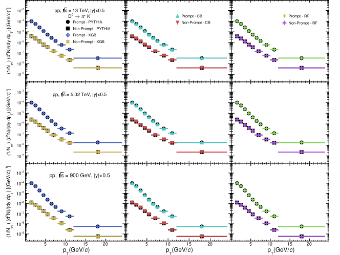
Figure 5: Transverse momentum spectra of prompt and nonprompt $D^{0}$ meson at three different energies predicted by three different machine-learning algorithms. The first row depicts the normalized prompt and nonprompt $D^{0}$ yields in $pp$ collisions at $\sqrt{s}=13~{}\rm{TeV}$. The second row presents the normalized yield at $\sqrt{s}=5.02~{}\rm{TeV}$, and the third row illustrates the normalized yield at $\sqrt{s}=900~{}\rm{GeV}$.

In Figure 3, the confusion matrix for target classes, such as prompt, nonprompt, and background, for different ML algorithms used in this study are shown. The confusion matrix, or error matrix, is an essential benchmark in understanding the model performance. We plot the fraction of true pair counts from PYTHIA8 in the $Y$-axis and the fraction of predicted pair counts from ML models in the $X$-axis. The numbers shown inside the boxes represent the corresponding fraction of $\pi K$ pairs. All three ML models are found to separate the background pairs with an accuracy of 100%. However, while separating prompt $D^{0}$ from the nonprompt ones, the XGBoost and CatBoost model have a better accuracy of 99% as compared to the Random Forest model, which has an accuracy of 97%. This means that the XGBoost and CatBoost models tag 1% of the nonprompt $D^{0}$ mesons as prompt $D^{0}$ while this is 3% in the Random Forest model. However, due to the imbalance between prompt and nonprompt classes, 1% of nonprompt $D^{0}$ do not make a significant contribution to the prompt $D^{0}$ meson counts. The magnitude of this mis-classification is not prominent, and we expect to accurately extract other physics variables of the predicted prompt and nonprompt $D^{0}$ mesons, which are further discussed in Section IV.

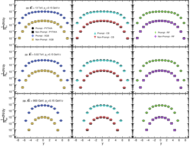
Figure 6: Rapidity spectra of prompt and nonprompt $D^{0}$ meson at different energies predicted by three different machine-learning algorithms. The first row shows the normalized prompt and nonprompt $D^{0}$ yield in $pp$ collisions at center-of-mass energy, $\sqrt{s}=13~{}\rm{TeV}$. The second row displays the normalized yield at $\sqrt{s}=5.02~{}\rm{TeV}$, while the third row represents the normalized yield at $\sqrt{s}=900~{}\rm{GeV}$.

The importance score, or feature importance, is a score assigned to each input feature based on how useful they are in making a model prediction. It depends on the number of times the input feature is used in splitting a node. By looking at the importance score, one can figure out the most and least relevant features of the dataset for a particular ML model. In Figure 4, we show the importance score of the input features, $m_{\pi K}$, $t_{z}$, DCA${}_{D^{0}}$, and $c\tau$. For all the three ML models, the input features $m_{\pi K}$ and DCA${}_{D^{0}}$possess the highest importance score. This signifies that these two input features carry the maximum information used in separating the background, prompt, and nonprompt classes. However, one can observe that the XGBoost model learns only from $m_{\pi K}$ and DCA${}_{D^{0}}$explicitly. In contrast, the Random Forest model learns mostly from DCA${}_{D^{0}}$, but also gives significant importance to $m_{\pi K}$ and $t_{z}$. The CatBoost model learns mostly from $m_{\pi K}$ and DCA${}_{D^{0}}$; however, still uses input from $t_{z}$ and $c\tau$ for splitting the nodes.

IV Results and Discussion

IV.1 Transverse momentum and rapidity spectra

Figure 5 shows the $p_{\rm{T}}$-differential yield of prompt and nonprompt $D^{0}$ meson in midrapidity, $|y|<0.5$, in $pp$ collisions at three different center-of-mass energies, i.e., $\sqrt{s}=13~{}\text{TeV}$ (upper), $\sqrt{s}=5.02~{}\text{TeV}$ (middle), and $\sqrt{s}=900~{}\text{GeV}$ (lower). We reconstruct $D^{0}$ meson through its hadronic decay channel, i.e., $D^{0}\rightarrow K^{-}\pi^{+}$. The plots include the predictions from XGBoost (left), CatBoost (center), and Random Forest (right). The PYTHIA8 generated spectra for the respective energies are also shown. All three ML models are trained with a minimum bias dataset of $pp$ collisions at $\sqrt{s}=13~{}\rm{TeV}$ simulated with PYTHIA8 and then applied to $pp$ collisions at lower collision energies. One can observe that the yield of nonprompt $D^{0}$ is significantly less in the whole $p_{\rm T}$ region, owing to the smaller production probability of beauty hadrons due to their higher masses. However, as one moves towards a higher $p_{\rm T}$ region, it can be seen that the $p_{\rm T}$-spectra curves from prompt and nonprompt $D^{0}$ mesons slightly approach each other. This indicates that the yield of nonprompt $D^{0}$ relative to the prompt $D^{0}$ meson increases with increase in $p_{\rm T}$. All three models are found to predict the normalized $D^{0}$ yield for energies $\sqrt{s}=5.02~{}\rm{TeV}$ and $\sqrt{s}=900~{}\rm{GeV}$ reasonably well. It is observed that the ML models are quite successful in predicting the $p_{\rm T}$-differential yield at different collision energies. Thus, they appear to retain the collision energy dependence. The ability of the models to learn and preserve the energy dependence of prompt and nonprompt $D^{0}$ production highlights their robustness and accuracy. This is primarily due to their learning is largely influenced by two factors, the invariant mass ($m_{\pi K}$) and the distance of the closest approach (DCA${}_{D^{0}}$), which are independent of $\sqrt{s}$.

Figure 6 shows the rapidity spectra of prompt and nonprompt $D^{0}$ reconstructed from candidates with $p_{\rm T}>0.15$ GeV/c in minimum bias $pp$ collisions at $\sqrt{s}=13~{}\rm{TeV}$ (upper), $\sqrt{s}=5.02~{}\rm{TeV}$ (middle), and $\sqrt{s}=900~{}\rm{GeV}$ (lower). The results from PYTHIA8, XGBoost, CatBoost, and Random Forest are shown. The energy dependence of the width of the rapidity spectra is noticeable, and the differences can be clearly observed comparing the highest and lowest center-of-mass energies. In addition, the width of the rapidity spectra of the prompt $D^{0}$ meson is always greater than that of the nonprompt case at any given energy. For $\sqrt{s}=13~{}\rm{TeV}$, the midrapidity region for the prompt $D^{0}$ seems flat in log-scale in the range, $|y|\lesssim 3$; however, this flat region for the prompt $D^{0}$ decreases with decreasing the collision energy. For $\sqrt{s}=5.02~{}\rm{TeV}$, the flat region confides in a slightly smaller rapidity range of $|y|\lesssim 2$. This region shrinks even more for $\sqrt{s}=900~{}\rm{GeV}$ where a smaller plateau exists only within $|y|\lesssim 1$. Moreover, this flat midrapidity plateau is much smaller for the nonprompt $D^{0}$ meson, as evident from the plots. The flat region is almost non-existent for $\sqrt{s}=900~{}\rm{GeV}$. However, it extends to a range of $|y|\lesssim 2$ for $\sqrt{s}=13~{}\rm{TeV}$. From Figs. 5 and 6, we notice that all the three ML models predict a similar level of accuracy in the yield of $D^{0}$ meson as a function of transverse momentum and rapidity. Consequently, beyond this point in text, for the sake of clarity in the plots, we will be only focusing on the predictions from the XGBoost model and compare it with PYTHIA8 results, since the XGBoost model shows the highest degree of accuracy compared to the Random Forest model in this scenario.

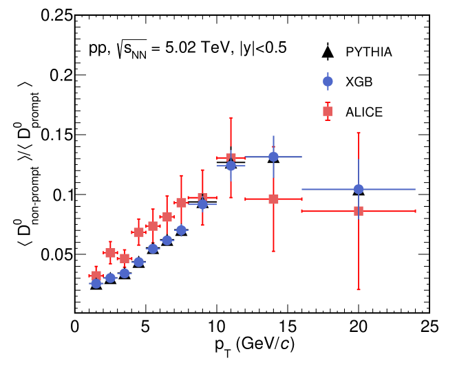
Figure 7: Nonprompt to prompt $D^{0}$ meson ratio in minimum bias $pp$ collisions at $\sqrt{s}=5.02~{}\rm{TeV}$ from PYTHIA8 compared with ALICE results and predictions from XGBoost [51].

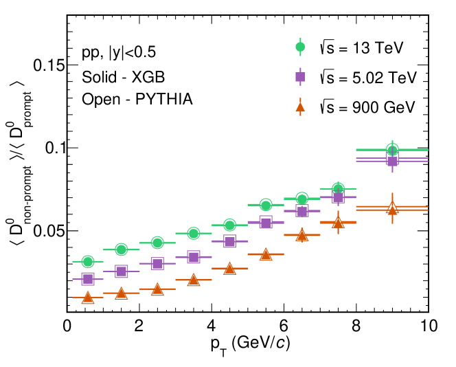
Figure 8: Nonprompt to prompt $D^{0}$ meson ratio for three different center-of-mass energies from PYTHIA8 compared with the predictions from XGBoost in minimum bias $pp$ collisions.

IV.2 Nonprompt to prompt ratio and self-normalized yield of $D^{0}$ meson

Figure 7 presents the ratio of nonprompt to prompt $D^{0}$ yield, at midrapidity, $|y|<0.5$ in minimum bias $pp$ collisions at $\sqrt{s}=5.02~{}\rm{TeV}$, as a function of $p_{\rm T}$. This ratio essentially tells us about the relative yield of $D^{0}$ mesons coming from beauty hadrons decays, compared to the direct charm hadron production. We compare the XGBoost predictions with the ALICE [51] results. From the plot, it is observed that PYTHIA8 underestimates the experimental results at lower-$p_{\rm T}$ and starts to approach the experimental results only towards the higher-$p_{\rm T}$ bins. However, the overall trend of PYTHIA8 is similar to that of the experimental findings. Again, the nonprompt to prompt $D^{0}$ yield ratio increases linearly up to $p_{\rm{T}}=12~{}\rm{GeV}/\textit{c}$. This indicates that the probability of charm hadron production from beauty decays increases linearly with $p_{\rm{T}}$. However, this linear trend holds good up to a certain $p_{\rm{T}}$ range. Similar results are also reported for charmonium states [47, 30]. However, the increase in nonprompt charmonium states as a function of $p_{\rm T}$ is much higher than that of the open-charm states  [30]. Moreover, for $p_{\rm{T}}>12~{}\rm{GeV}/\textit{c}$, the ALICE data is uncertain with larger error bars, and the trend appears to become independent of $p_{\rm{T}}$. The predictions from XGBoost are found to be inline both qualitatively and quantitatively with the PYHTIA8 true values.

Figure 8 shows the nonprompt to prompt $D^{0}$ ratio in minimum bias $pp$ collisions at three different center-of-mass energies, i.e., $\sqrt{s}=13~{}\rm{TeV}$, $5.02~{}\rm{TeV}$, and $900~{}\rm{GeV}$. One can clearly notice the increase in the ratio with increasing $p_{\rm T}$ across all the collision energies. However, we observe an energy-dependent hierarchy in the ratio, as the charm production from beauty decays compared to the direct charm production is minimum for $\sqrt{s}=900~{}\rm{GeV}$ and maximum for the case of $\sqrt{s}=13~{}\rm{TeV}$. In addition, towards higher $p_{\rm{T}}$, we see the rise of the ratio, indicating an increase in the beauty hadron production leading to an enhancement of the nonprompt yield.

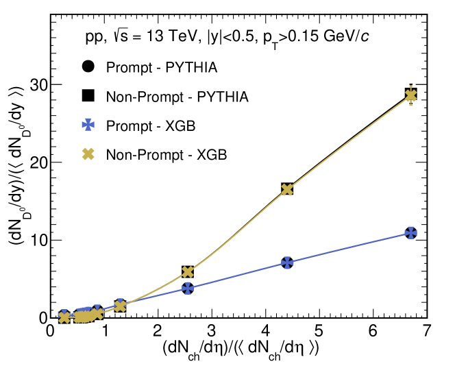
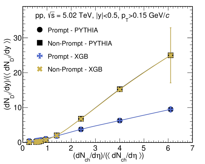
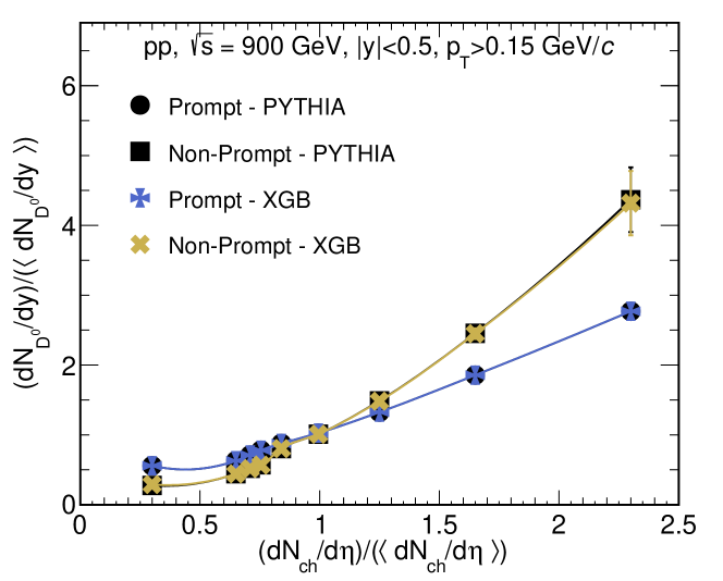
Figure 9: Self-normalized $p_{\rm{T}}$ integrated prompt and nonprompt $D^{0}$ meson yield at midrapidity ($|y|<0.5$) as a function of normalized charged-particle multiplicity in minimum bias $pp$ collisions at $\sqrt{s}=13~{}\rm{TeV}$ (upper), $\sqrt{s}=5.02~{}\rm{TeV}$ (middle), and $\sqrt{s}=900~{}\rm{GeV}$ (lower). The charged-particle multiplicity is obtained within the ALICE-V0 detector acceptance.

Figure 9 shows the self-normalized $p_{\rm{T}}$ integrated yield of prompt and nonprompt $D^{0}$ meson in midrapidity ($|y|<0.5$) as a function of normalized charged-particle multiplicity in minimum bias $pp$ collisions at $\sqrt{s}=13~{}\rm{TeV}$ (upper), $\sqrt{s}=5.02~{}\rm{TeV}$ (middle), and $\sqrt{s}=900~{}\rm{GeV}$ (lower). The charged-particle multiplicity is obtained within the ALICE-V0 detector acceptance which covers the intervals $2.8<\eta<5.1$ (V0A) and $-3.7<\eta<-1.7$ (V0C). The charged-particle multiplicity used for the normalized yield selection, is the coincidence signal of V0A and V0C. The selection of $D^{0}$ meson and charged particle multiplicity in two different rapidity regions is to reduce the autocorrelation bias. The results include PYTHIA8 values and the prediction from the XGBoost model. We observe an almost linear rise for the prompt $D^{0}$ meson with respect to the charged particle multiplicity for all the three collision energies. However, the self-normalized yield of nonprompt $D^{0}$ is significantly enhanced towards higher collision energy and follows a faster than linear trend with increasing charged-particle multiplicity. A similar trend for charmonium states (i.e. $J/\psi$) has been reported in the literature using PYTHIA8 [30]. For the plots shown here, XGBoost predictions closely follow the PYTHIA8 curves.

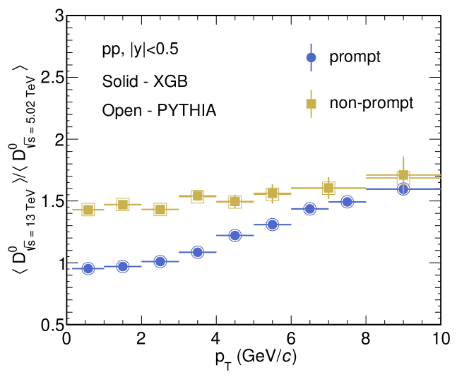
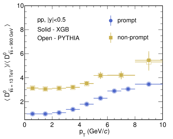
Figure 10: Ratio of $D^{0}$ yield in $pp$ collisions at $\sqrt{s}=13$ and 5.02 TeV (upper) and at $\sqrt{s}=13~{}\rm{TeV}$ and $\sqrt{s}=900~{}\rm{GeV}$ (lower) as a function of $p_{\rm{T}}$.

Finally, we study the role of center-of-mass energy in $D^{0}$ meson production. We estimate the ratio of $D^{0}$ yield in two different energies. In the upper panel of Fig. 10, we plot the ratio of $D^{0}$ yield in $\sqrt{s}=13~{}\rm{TeV}$ to $\sqrt{s}=5.02~{}\rm{TeV}$. Here, for the prompt case, we notice a clear increase in the ratio with an increasing $p_{\rm{T}}$. However, we observe a flat trend throughout the whole $p_{\rm{T}}$ range for the nonprompt case. A similar trend has been observed recently at ALICE [52]. In addition, a higher value of the nonprompt than prompt ratio shows the abundant production of beauty hadrons at higher center-of-mass energy. In the lower panel, we plot the same ratio between $\sqrt{s}=13~{}\rm{TeV}$ and $\sqrt{s}=900~{}\rm{GeV}$. We observe a similar increasing trend for the prompt case, however, for the case of nonprompt, because of a significant difference in collision energy, a rising trend is observed as a function of transverse momentum. Furthermore, due to the higher difference in the center-of-mass energy, the absolute values of the ratio go up (lower panel compared to the upper panel of Fig. 10). Interestingly, XGBoost is able to predict the PYTHIA8 trends with very high accuracy.

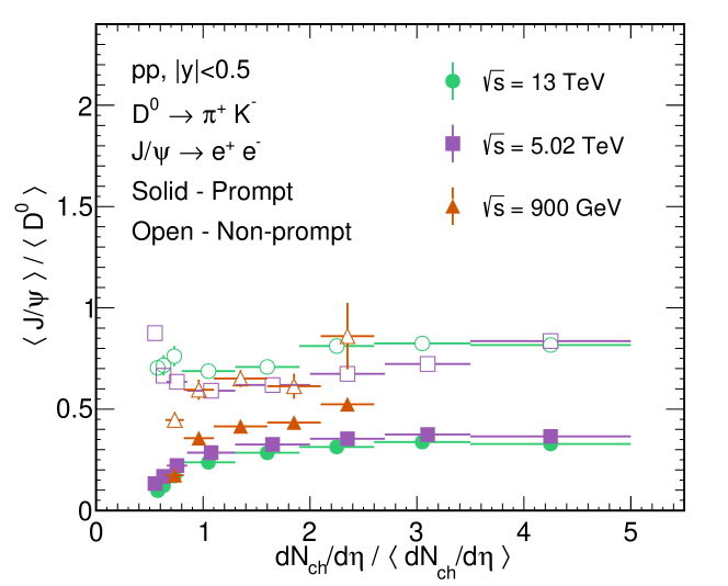
Figure 11: Upper: Normalized $J/\psi$ yield to $D^{0}$ yield ratio as a function of $p_{\rm T}$ in $pp$ collisions at $\sqrt{s}=13$ and 5.02 TeV and $\sqrt{s}=900~{}\rm{GeV}$. Lower: $p_{\rm{T}}$ integrated normalized $J/\psi$ yield to $D^{0}$ yield ratio as a function of normalized charged-particle multiplicity estimated within ALICE-V0 acceptance.

IV.3 Ratio of charmonium to open-charm state

It is interesting to study the production dynamics of charmonium states relative to open-charm states. In Fig. 11, on the upper panel, the normalized $J/\psi$ to $D^{0}$ yield as a function of $p_{\rm T}$ is shown in minimum bias $pp$ collisions. To understand the contribution coming from the charm and beauty sectors, we estimate the ratio of prompt $J/\psi$ to prompt $D^{0}$, as well as the ratio of nonprompt $J/\psi$ to nonprompt $D^{0}$. We observe similar trends for the prompt and nonprompt cases. A rise in the ratio can be seen up to $p_{\rm{T}}\simeq 5~{}\rm{GeV}/\textit{c}$ and it shows a flat trend beyond $5~{}\rm{GeV}/\textit{c}$. This trend is universal for all center-of-mass energies. It indicates that the relative number of $J/\psi$ increases as compared to $D^{0}$, with an increase in $p_{\rm T}$. One can notice that the ratio of nonprompt $J/\psi$ to nonprompt $D^{0}$ is higher than one, indicating a higher number of nonprompt $J/\psi$ compared to nonprompt $D^{0}$. Assuming that the same beauty hadrons contribute to the production of nonprompt $J/\psi$ and nonprompt $D^{0}$ mesons, $\langle J/\psi\rangle/\langle D^{0}\rangle>1$ for nonprompt case indicates that a beauty hadron would more likely to decay into a $J/\psi$ than to a $D^{0}$ mesons. In other words, the branching fraction of beauty hadrons decaying into $J/\psi$ is higher than their decay to $D^{0}$. However, as expected, the ratio of prompt $J/\psi$ to prompt $D^{0}$ is less than one, owing to the larger mass of $J/\psi$. In the lower panel, we present the $\langle J/\psi\rangle/\langle D^{0}\rangle$ as a function of normalised charged-particle multiplicity. Here, we observe two different trends for the prompt and nonprompt cases. We notice the nonprompt $J/\psi$ to $D^{0}$ ratio remains almost independent of normalised charged-particle multiplicity. However, for the prompt case, we notice a slight increase and then a flat trend in the ratio with the increase in the normalised charged-particle multiplicity. Additionally, there is a noticeable ordering in the prompt $J/\psi$ to $D^{0}$ ratio, where the ratio increases with a decrease in collision energy. This trend is consistent throughout all the charged-particle multiplicities.

V Summary

In this paper, we present a novel method for track-level identification and segregation of the prompt and nonprompt $D^{0}$ meson from the background pion-kaon pairs using machine learning algorithms. We use experimentally measurable topological variables as inputs, which include the invariant mass ($m_{\pi K}$), pseudoproper time ($t_{z}$), pseudoproper decay length ($c\tau$), and distance of closest approach (DCA${}_{D^{0}}$). We train the XGBoost, CatBoost, and Random Forest models with data generated using PYTHIA8 for $pp$ collisions at $\sqrt{s}=13~{}\rm{TeV}$. The XGBoost and CatBoost models show an accuracy up to 99% in separating prompt and nonprompt $D^{0}$ mesons; however, the Random Forest model shows an accuracy of 97%. The models are efficient and robust enough to predict the results even at lower collision energies: $\sqrt{s}=5.02~{}\rm{TeV}$ and $\sqrt{s}=900~{}\rm{GeV}$ in the complete transverse momentum and pseudorapidity region.

Also, to understand the production of prompt and nonprompt $D^{0}$ meson, we study the nonprompt to prompt ratio of $D^{0}$ yield as a function of transverse momenta. Furthermore, we study the self-normalized yield of $D^{0}$ meson, where we observe a nonlinear rising trend for the nonprompt $D^{0}$ as a function of normalized charged particle multiplicity. In addition, we have incorporated predictions and results from several collision energies, which not only serve as a benchmark for the predictions from the machine learning models but also provide a collision energy dependence study of prompt and nonprompt $D^{0}$ mesons. Finally, we explore the relative production of charmonium, $J/\psi$ to open-charm, $D^{0}$ states as a function of transverse momenta and charged-particle multiplicity. In all these studies, the predictions from XGBoost match the PYTHIA8 values quite well. This method has an advantage over the conventional methods as it can perform unbinned measurements for both prompt and nonprompt $D^{0}$ by directly tagging the decay daughters.

The ongoing ALICE Run 3 data taking with high luminosity and better detection capabilities would pave way for several precise measurements for the charm and beauty sector. The separation of charm hadron topological production into prompt and nonprompt ones allows us to explore the beauty sector. The ability to separate the contribution from the beauty sector gives us a better understanding of the dynamics of the charmed hadron production, their interaction with the QGP, and the properties of the QCD medium. The use of machine learning algorithms can help us replace the traditional fitting procedures with improved track-level identification of the prompt and nonprompt production of charm hadrons. This study demonstrates the efficiency of using machine learning techniques in topological separation of open charm mesons in an experiment-like scenario using the track-level inputs, the enhancement of which (prompt open charm) is considered as a signature of QGP. The production dynamics of prompt vs non-prompt charmonium and open charm at the LHC energies using the ALICE upgarde would provide a test bench for QCD and the study of multihadron production dynamics extending to the beauty sector at the subatomic level.

VI Acknowledgements

K. G. acknowledges the financial support from the Prime Minister’s Research Fellowship (PMRF), Government of India. S.P. acknowledges the doctoral fellowships from the University Grants Commission (UGC), Government of India. The authors acknowledge the DAE-DST, Government of India funding under the Mega-Science Project—“Indian participation in the ALICE experiment at CERN” bearing Project No. SR/MF/PS-02/2021-IITI (E-37123). The authors sincerely acknowledge the usage of resources of the LHC grid Tier-3 computing facility at IIT Indore.

Appendix

For a better understanding of the model training, we have shown the learning rate of the XGBoost and the CatBoost model in Fig. 12. It serves as a pivotal tool for understanding the model’s learning trajectory and performance over the course of training. The learning curves enable us to diagnose issues of underfitting or overfitting, hence ensuring the model’s robustness. Moreover, they assist in the process of hyperparameter tuning, thereby optimizing the model’s performance. Lastly, they provide insights into the efficiency of the training process, potentially conserving computational resources.

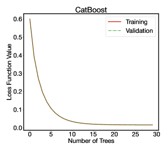
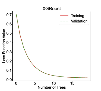
Figure 12: Learning curve of Catboost and XGBoost.

However, the Random Forest model, being an ensemble of Decision Trees, does not learn in an iterative manner. Each tree in the forest is built independently of the others. Therefore, there is no concept of iterations during which the model progressively learns and improves. Thus, it is not possible to plot a learning curve for the random forest method, unlike for the XGBoost and the CatBoost models.

References

- [1] F. M. Liu and S. X. Liu, Phys. Rev. C 89, 034906 (2014).
- [2] J. Adam et al. [ALICE Collaboration], JHEP 03, 081 (2016).
- [3] D. Acosta et al. [CDF Collaboration], Phys. Rev. Lett. 91, 241804 (2003).
- [4] S. Acharya et al. [ALICE Collaboration], JHEP 10, 174 (2018).
- [5] S. Acharya et al. [ALICE Collaboration], Phys. Lett. B 846, 137561 (2023).
- [6] B. Abelev et al. [ALICE Collaboration], Phys. Rev. Lett. 111, 102301 (2013).
- [7] S. Acharya et al. [ALICE Collaboration], Phys. Lett. B 827, 136986 (2022).
- [8] L. Adamczyk et al. [STAR Collaboration], Phys. Rev. Lett. 118, 212301 (2017).
- [9] A. M. Sirunyan et al. [CMS Collaboration], Phys. Rev. Lett. 121, 082301 (2018).
- [10] A. M. Sirunyan et al. [CMS Collaboration], Phys. Lett. B 816, 136253 (2021).
- [11] A. Tumasyan et al. [CMS Collaboration], Phys. Lett. B 850, 138389 (2024).
- [12] S. Acharya et al. [ALICE Collaboration], Eur. Phys. J. C 83, 1123 (2023).
- [13] A. M. Sirunyan et al. [CMS Collaboration], Phys. Lett. B 782, 474 (2018).
- [14] S. Acharya et al. [ALICE Collaboration], JHEP 01, 174 (2022).
- [15] D. Bowser-Chao and D. L. Dzialo, Phys. Rev. D 47, 1900 (1993).
- [16] P. Chiappetta, P. Colangelo, P. De Felice, G. Nardulli and G. Pasquariello, Phys. Lett. B 322, 219 (1994).
- [17] S. A. Bass, A. Bischoff, J. A. Maruhn, H. Stoecker and W. Greiner, Phys. Rev. C 53, 2358 (1996).
- [18] R. Haake [ALICE Collaboration], PoS EPS-HEP2019 (2020), 312
- [19] S. Acharya et al. [ALICE Collaboration], Phys. Lett. B 849, 138412 (2024).
- [20] M. Paganini [ATLAS Collaboration], J. Phys. Conf. Ser. 1085, 042031 (2018).
- [21] G. Aad et al. [ATLAS Collaboration], Phys. Rev. Lett. 125, 131801 (2020).
- [22] A. M. Sirunyan et al. [CMS Collaboration], JINST 15 (2020), P06005.
- [23] Ł. K. Graczykowski et al. [ALICE Collaboration], JINST 17 (2022), C07016.
- [24] A. Ryzhikov et al. [LHCb Collaboration], J. Phys. Conf. Ser. 2438, 012119 (2023).
- [25] N. Mallick, S. Tripathy, A. N. Mishra, S. Deb and R. Sahoo, Phys. Rev. D 103, 094031 (2021).
- [26] X. Zhang, Y. Huang, W. Lin, X. Liu, H. Zheng, R. Wada, A. Bonasera, Z. Chen, L. Chen and J. Han, et al. Phys. Rev. C 105, 034611 (2022).
- [27] N. Mallick, S. Prasad, A. N. Mishra, R. Sahoo and G. G. Barnaföldi, Phys. Rev. D 105, 114022 (2022).
- [28] N. Mallick, S. Prasad, A. N. Mishra, R. Sahoo and G. G. Barnaföldi, Phys. Rev. D 107, 094001 (2023).
- [29] H. Hirvonen, K. J. Eskola and H. Niemi, Phys. Rev. C 108, 034905 (2023).
- [30] S. Prasad, N. Mallick and R. Sahoo, Phys. Rev. D 109, 014005 (2024).
- [31] [ATLAS Collaboration], “Electron Identification with a Convolutional Neural Network in the ATLAS Experiment,” ATL-PHYS-PUB-2023-001.
- [32] T. Sjostrand, S. Mrenna and P. Z. Skands, JHEP 05, 026 (2006).
- [33] Pythia8 online manual: https://pythia.org/manuals/pythia8215/Welcome.html (Accessed on: 05 Apr 2024)
- [34] R. Corke and T. Sjostrand, JHEP 03, 032 (2011).
- [35] K. Aamodt et al. [ALICE Collaboration], Eur. Phys. J. C 71, 1594 (2011).
- [36] S. Acharya et al. [ALICE Collaboration], Phys. Rev. Lett. 128, 012001 (2022).
- [37] Available Online: https://machine-learning-tutorial-abi.readthedocs.io/en/latest/index.html (Accessed on: 05 Apr 2024)
- [38] S. Acharya et al. [ALICE Collaboration], Phys. Rev. D 108, 112003 (2023).
- [39] A. Tumasyan et al. [CMS Collaboration], JHEP 11, 225 (2021).
- [40] R. Aaij et al. [LHCb Collaboration], JHEP 03, 159 (2016) [erratum: JHEP 09, 013 (2016); erratum: JHEP 05, 074 (2017)].
- [41] Available Online: https://catboost.ai/en/docs/ (Accessed on: 05 Apr 2024)
- [42] L. Prokhorenkova et al. CatBoost: unbiased boosting with categorical features, [arXiv:1760.09516[cs.LG]].
- [43] Gilles Louppe Understanding Random Forests: From Theory to Practice [arXiv:1407.7502 [stat.ML]]
- [44] Tianqi Chen and Carlos Guestrin XGBoost: A Scalable Tree Boosting System [arXiv:1603.02754 [cs.LG]]
- [45] Available Online: https://xgboost.readthedocs.io/en/stable/ (Accessed on: 05 Apr 2024)
- [46] R. Aaij et al. [LHCb Collaboration], Phys. Lett. B 774, 159 (2017).
- [47] S. Acharya et al. [ALICE Collaboration], JHEP 03, 190 (2022).
- [48] J. Adam et al. [STAR Collaboration], Phys. Rev. C 99, 034908 (2019).
- [49] R. L. Workman et al. [Particle Data Group], PTEP 2022, 083C01 (2022).
- [50] N. V. Chawla, K. W. Bowyer, L. O. Hall and W. P. Kegelmeyer, J. Artif. Intell. Res. 16, 321 (2002).
- [51] S. Acharya et al. [ALICE Collaboration], JHEP 05, 220 (2021).
- [52] S. Acharya et al. [ALICE Collaboration], [arXiv:2402.16417 [hep-ex]].