Hierarchical Fault-Tolerant Coverage Control for an Autonomous Aerial Agent

Abstract

Fault-tolerant coverage control involves determining a trajectory that enables an autonomous agent to cover specific points of interest, even in the presence of actuation and/or sensing faults. In this work, the agent encounters control inputs that are erroneous; specifically, its nominal controls inputs are perturbed by stochastic disturbances, potentially disrupting its intended operation. Existing techniques have focused on deterministically bounded disturbances or relied on the assumption of Gaussian disturbances, whereas non-Gaussian disturbances have been primarily been tackled via scenario-based stochastic control methods. However, the assumption of Gaussian disturbances is generally limited to linear systems, and scenario-based methods can become computationally prohibitive. To address these limitations, we propose a hierarchical coverage controller that integrates mixed-trigonometric-polynomial moment propagation to propagate non-Gaussian disturbances through the agent’s nonlinear dynamics. Specifically, the first stage generates an ideal reference plan by optimising the agent’s mobility and camera control inputs. The second-stage fault-tolerant controller then aims to follow this reference plan, even in the presence of erroneous control inputs caused by non-Gaussian disturbances. This is achieved by imposing a set of deterministic constraints on the moments of the system’s uncertain states.

1 Introduction

Coverage planning in autonomous systems (Tan2021; Papaioannou et al. (2022); Papaioannou2023CDC) refers to the problem of designing a trajectory or a series of actions for an autonomous agent to ensure that it covers a specified area or a set of points of interest, while at the same time optimising a particular mission objective.

Recently, unmanned aerial vehicle (UAV) -based systems have been increasingly applied to various application domains as shown in ZachariaMED; PapaioannouMED; Soleymani2023; PapaioannouIROS2021 including coverage control, as highlighted in Cabreira et al. (2019); PapaioannouTAES; PapaioannouICUAS2022. However, the majority of these approaches, primarily focus on covering 2D planar areas. These methods often employ simple geometric patterns, such as back-and-forth or zig-zag motions, which are not easily adaptable to 3D environments, and predominantly utilize UAVs with fixed, non-controllable sensors.

In addition, in specific application domains, such as emergency response and critical infrastructure inspection, fault-tolerant coverage control (FTCC) is imperative. The primary goal of fault-tolerant control (FTC) is to sustain system performance close to the desired level despite various types of faults, including actuation and sensing faults. Over the last years, the field of FTC has gained considerable attention (zhang2008bibliographical). Numerous FTC methods, including both passive and active approaches, have been proposed in the literature (jiang2012fault) for linear and nonlinear systems to address a variety of faults. However, several challenges remain unresolved, particularly in dealing with faults arising from random disturbances, such as erroneous control inputs caused by stochastic and potentially non-Gaussian disturbances.

Existing methodologies usually employ deterministically bounded disturbances (Mayne et al. (2005)) or are based on linear-Gaussian assumptions regarding the disturbances affecting the system (Vitale et al. (2022); Dai et al. (2019)). While fault-tolerant and robust methods accommodating nonlinear system dynamics (Lew et al. (2020)) have been developed, they often presuppose Gaussian disturbances Papaioannou2023unscented. In contrast, to handle non-Gaussian disturbances, scenario-based stochastic control methods have been introduced (Summers (2018); Calafiore and Fagiano (2013)), however, these are generally constrained to linear systems.

To address these limitations, we propose in this work a fault-tolerant hierarchical coverage controller. It accounts for stochastic non-Gaussian disturbances affecting the nominal control inputs of an autonomous UAV agent. Consequently, these disturbances propagate through the agent’s nonlinear dynamical model, affecting its desired operation. The proposed approach allows for the accommodation of these disturbances, thereby facilitating the generation of fault-tolerant coverage plans.

2 Preliminaries

2.1 Agent Dynamical Model

In this study, we focus on an autonomous UAV agent whose state at time-step $t$ is represented by $\boldsymbol{x}_{t}\in\mathcal{X}\subset\mathbb{R}^{4}$. This agent operates within a bounded 3D surveillance area, $\mathcal{A}\subset\mathbb{R}^{3}$, and follows the stochastic discrete-time dynamical model $\boldsymbol{x}_{t}=f(\boldsymbol{x}_{t-1},\boldsymbol{u}_{t-1},\boldsymbol{\omega}_{t-1})$, outlined below:

$$x_{t} =x_{t-1}+\Delta_{t}(u^{\nu}_{t-1}+\omega^{\nu}_{t-1})\cos(\psi_{t-1}),$$ (1a)

$$y_{t} =y_{t-1}+\Delta_{t}(u^{\nu}_{t-1}+\omega^{\nu}_{t-1})\sin(\psi_{t-1}),$$ (1b)

$$z_{t} =z_{t-1}+\Delta_{t}(u^{z}_{k-1}+\omega^{z}_{k-1}),$$ (1c)

$$\psi_{t} =\psi_{t-1}+\Delta_{t}(u^{\psi}_{t-1}+\omega^{\psi}_{t-1}).$$ (1d)

Here, $\boldsymbol{x}_{t}=[x_{t},y_{t},z_{t},\psi_{t}]^{\top}$ represents the agent’s position $(x_{t},y_{t},z_{t})$ and orientation $(\psi_{t})$, i.e., yaw, in 3D Cartesian coordinates. The control input vector $\boldsymbol{u}_{t}=[u^{\nu}_{t},u^{z}_{t},u^{\psi}_{t}]^{\top}\in\mathcal{U}$ comprises the horizontal and vertical velocities $(u^{\nu}_{t},u^{z}_{t})$, and the yaw rate $(u^{\psi}_{t})$, and $\Delta_{t}$ denotes the sampling interval. The term $\boldsymbol{\omega}_{t}=[\omega^{\nu}_{t},\omega^{z}_{t},\omega^{\psi}_{t}]^{\top}$ represents random disturbances acting on the agent’s nominal control inputs, thereby affecting its normal operation.

2.1.1 Assumption 1:

The disturbance term $\boldsymbol{\omega}_{t}$ is a probabilistic process noise vector consisting of independent components, i.e., random variables, which: a) can follow different probability density functions (potentially non-Gaussian), and b) have finite moments of order $\alpha\in\mathbb{N}$.

2.2 Agent Sensing Model

The UAV agent is outfitted with a gimballed camera exhibiting a limited field-of-view (FOV), and rotation capabilities. The camera FOV is modelled as a regular right pyramid with four triangular sides and a rectangular base. The optical center of the camera, is located at the pyramid’s apex, directly above the FOV base’s centroid. The dimensions of the FOV’s rectangular base, namely its length and width are denoted as $\ell_{f}$, and $w_{f}$ respectively, and the camera’s observation range is denoted as $h_{f}$ (i.e., pyramid’s height). The camera’s initial pose (i.e., the vertices of the FOV) are given by the 3-by-5 matrix $C_{0}$, as follows:

$$C_{0}=\begin{bmatrix}h_{f}&h_{f}&h_{f}&h_{f}&0\\ w_{f}/2&w_{f}/2&-w_{f}/2&-w_{f}/2&0\\ \ell_{f}/2&-\ell_{f}/2&-\ell_{f}/2&\ell_{f}/2&0\\ \end{bmatrix},$$ (2)

where the camera’s optical axis i.e., the line connecting the base’s centroid and the pyramid’s apex, of length $h_{f}$, aligns parallel to the $zy$-plane’s normal. At time-step $t$ the camera’s FOV can be rotated through two sequential rotations i.e., firstly, a rotation by an angle $\phi^{y}$ around the $y$-axis, and secondly, a rotation $\phi^{z}$ around the $z$-axis as: $C^{i}_{t}(\phi^{y},\phi^{z})=R_{z}(\phi^{z})R_{y}(\phi^{y})C^{i}_{0},\forall i\in\{1,..,5\}$, where $C^{i}_{0}$ denotes the $i_{\text{th}}$ column of the matrix $C_{0}$, $C^{i}_{t}(\phi^{y},\phi^{z})$ refers to the FOV vertex after rotation, as parameterized by the angles $\phi^{y}$ and $\phi^{z}$. The matrices $R_{y}(a)$ and $R_{z}(a)$ denote the fundamental 3-by-3 rotation matrices, which are used to rotate a vector by an angle $a$ around the $y$-axis and $z$-axis, respectively. Finally, the pair of rotation angles $\{\phi^{y},\phi^{z}\}\in\mathcal{M}$ is taken from the finite set $\mathcal{M}$ of all admissible camera rotations (i.e., pairwise combination of angles). In other words, the camera FOV can acquire at each time-step $t$, $1$ out of $|\mathcal{M}|$ possible configurations.

2.3 Points of Interest

In this study, we consider the surface area $\partial O$ of an object of interest $O$, to have been triangulated into a 3D mesh $\mathcal{K}=\{K_{1},..,K_{|\mathcal{K}}|\}$ composed of a finite number $|\mathcal{K}|$ of triangular facets $K\in\mathbb{R}^{3\times 3}$, where $|\cdot|$ signifies the set cardinality. The points of interest, i.e., the points that need to be covered by the agent’s camera, are defined as the centroid points of a specified subset of facets $\tilde{\mathcal{K}}\subseteq\mathcal{K}$ on the object’s surface area. The centroid point of facet $K\in\tilde{\mathcal{K}}$ will be denoted hereafter as $\boldsymbol{c}_{K}\in\mathbb{R}^{3}$, and the set of all centroid points to be covered as $\tilde{\mathcal{K}}_{c}$.

3 Robust Hierarchical Coverage Control

The problem tackled in this work can be stated as follows: Given a rolling finite planning horizon of length $T$ time-steps, find the UAV’s joint mobility i.e., $\boldsymbol{u}_{t+\tau|t}$, and camera i.e., $\{\phi^{y},\phi^{z}\}_{t+\tau|t}$ control inputs for $\forall\tau\in\{0,..,T-1\}$ which maximise the coverage of the points of interest $\boldsymbol{c}_{K}\in\tilde{\mathcal{K}}_{c}$ on the object’s surface area.

To address this problem, it’s important to recognize that the agent’s state, $\boldsymbol{x}_{t}$, is a multivariate random variable due to random disturbances affecting the system. This uncertainty extends to the state of the camera’s Field of View (FOV), making the coverage task inherently non-deterministic. To tackle this challenge robustly, we aim to ensure that the points of interest are covered with a certain probability $1-\epsilon$.

In this section, we show how we have addressed the above challenges by designing a hierarchical fault-tolerant coverage controller. In the first stage (i.e., Sec. 3.1), the problem is reformulated as a disturbance-free rolling horizon model predictive control problem (MPC), generating finite-length look-ahead coverage plans. In the second stage (i.e., Sec. 3.2), a fault-tollerant controller is developed, employing exact uncertainty propagation techniques to propagate the disturbance through the agent’s dynamics. This allows for the computation of constraints on the moments of the agent’s uncertain states, ensuring fault-tolerant coverage control at specified probability levels.

3.1 Stage-1: Coverage Reference Plan

The first-stage controller, as formulated in (3), is designed as a rolling horizon MPC. In this setup, the agent computes finite-length look-ahead coverage trajectories $\boldsymbol{x}^{1}_{t+\tau+1|t}$ for $\tau\in\{0,..,T-1\}$. [h]

$$~{}~{}\underset{\{\boldsymbol{u^{1}},\boldsymbol{b^{GC}}\}}{\min}~{}\mathcal{J}^{1}=\mathcal{J}^{1}_{\text{GC}}+w\mathcal{J}^{1}_{\text{CE}}$$ (3a)

subject to: $$\tau\in\{0,..,T-1\}$$

$$\boldsymbol{x}^{1}_{t+\tau+1|t}=\Phi\boldsymbol{x}^{1}_{t+\tau|t}+\Gamma\boldsymbol{u}^{1}_{t+\tau|t}, \forall\tau$$ (3b)

$$\boldsymbol{x}^{1}_{t|t}=\boldsymbol{x}^{1}_{t|t-1},$$ (3c)

$$b^{\text{G}}_{\kappa,t+\tau+1|t}=1\iff\text{pos}(\boldsymbol{x}^{1}_{t+\tau+1|t})\in\bigtriangleup(S_{\kappa}), \forall\kappa,\tau$$ (3d)

$$\sum_{\tau}b^{\text{G}}_{\kappa,t+\tau+1|t}\leq 1, \forall\kappa$$ (3e)

$$\hat{b}^{\text{G}}_{\kappa,t+\tau+1|t}\leq b^{\text{G}}_{\kappa,t+\tau+1|t}+V(\kappa), \forall\kappa,\tau$$ (3f)

$$C_{m}=R_{z}(\phi^{z})R_{y}(\phi^{y})C_{0}, \forall\{\phi^{z},\phi^{y}\}\in\mathcal{M}$$ (3g)

$$\hat{C}_{m,t+\tau+1|t}=C_{m}+\text{pos}(\boldsymbol{x}^{1}_{t+\tau+1|t}), \forall m,\tau$$ (3h)

$$b^{\text{FOV}}_{\kappa,m,t+\tau+1|t}=1\iff\boldsymbol{c}_{K}\in\bigtriangleup(\hat{C}_{m,t+\tau+1|t}), \forall\kappa,m,\tau$$ (3i)

$$\sum_{\kappa}\sum_{m}b^{\text{FOV}}_{\kappa,m,t+\tau+1|t}\leq 1, \forall\tau$$ (3j)

$$\hat{b}^{\text{FOV}}_{\kappa,m,t+\tau+1|t}\leq b^{\text{FOV}}_{\kappa,m,t+\tau+1|t}+V(\kappa), \forall\kappa,m,\tau$$ (3k)

$$b^{GC}_{\kappa,m,t+\tau+1|t}=\hat{b}^{\text{G}}_{\kappa,t+\tau+1|t}\wedge\hat{b}^{\text{FOV}}_{\kappa,m,t+\tau+1|t}, \forall\kappa,m,\tau$$ (3l)

In (3), we generate an ideal coverage reference plan based on simplified linear dynamics of the agent in a disturbance free setting, as shown in (3b), where the matrices $\Phi$ and $\Gamma$ are given by:

$$\Phi=\begin{bmatrix}\boldsymbol{1}_{3\times 3}&\Delta_{t}^{1}\boldsymbol{1}_{3\times 3}\\ \boldsymbol{0}_{3\times 3}&\boldsymbol{1}_{3\times 3}\end{bmatrix},~{}\Gamma=\begin{bmatrix}\boldsymbol{0}_{3\times 3}\\ \boldsymbol{1}_{3\times 3}\end{bmatrix}.$$ (4)

The matrices $\boldsymbol{1}_{3\times 3}$ and $\boldsymbol{0}_{3\times 3}$ denote the 3-by-3 identity and zero matrices respectively, and $\Delta_{t}^{1}$ denotes the sampling rate. The agent’s state $\boldsymbol{x^{1}_{t}}$ is composed of position and velocity components in 3D Cartesian coordinates, and the control input vector $\boldsymbol{u^{1}_{t}}$ represents the velocity components in 3D coordinates.

3.1.1 Assumption 2:

For each point of interest $\boldsymbol{c}_{K}\in\tilde{\mathcal{K}}_{c}$, there is an associated region of interest $S_{\kappa}\subset\mathcal{A}$ (where $\kappa$ is the index used to identify $\boldsymbol{c}_{K}$). When the agent resides within this region (i.e., $\text{pos}(\boldsymbol{x}_{t})\in S_{\kappa}$), there exist at least one configuration of the camera FOV $m\in\{1,..,|\mathcal{M}|\}$ that can ensure the coverage of $\boldsymbol{c}_{K}$. $S_{\kappa}$ is identified as a sphere with radius $s_{r}$ centered at $\boldsymbol{\bar{s}}_{\kappa}=\ell\boldsymbol{a}^{S}_{\kappa}+\boldsymbol{c}_{K}$, where $\ell$ is a appropriately selected distance, and $\boldsymbol{a}^{S}_{\kappa}$ is the outward unit normal vector to the facet $K\in\tilde{\mathcal{K}}$ which has as its centroid point, the point of interest $\boldsymbol{c}_{K}$.

UAV guidance through the regions of interest: We utilize the binary variable $b^{\text{G}}_{\kappa,t+\tau+1|t}$ in (3d) to identify whether the agent’s position $\text{pos}(\boldsymbol{x}^{1}_{t+\tau+1|t})$ at the time-step $t+\tau+1|t$ inside the planning horizon (hereafter abbreviated as $\tau$) resides inside the convex-hull of the $\kappa_{\text{th}}$ sphere $S_{\kappa}$, associated with the point of interest $\boldsymbol{c}_{K}$. To implement this functionality with linear inequalities, we first linearise $S_{\kappa}$ by approximating it with the inscribed dodecahedron as in PapaioannouTMC2023. Subsequently, we can identify the presence of the agent inside the dodecahedron as shown below:

$$\text{dot}(\boldsymbol{a}_{i,\kappa},\text{pos}(\boldsymbol{x}^{1}_{\tau}))+\bar{b}^{\text{G}}_{i,\kappa,\tau}(M-\beta_{i,\kappa})\leq M,$$ (5a)

$$12b^{\text{G}}_{\kappa,\tau}-\sum_{i=1}^{12}\bar{b}^{\text{G}}_{i,\kappa,\tau}\leq 0$$ (5b)

where $\text{dot}(\boldsymbol{a}_{i,\kappa},\boldsymbol{x})=\beta_{i,\kappa}$ describes the equation of the plane which contains the $i_{\text{th}}$ facet of the $\kappa_{\text{th}}$ dodecahedron associated with the point of interest $\boldsymbol{c}_{K}$, $\boldsymbol{x}\in\mathbb{R}^{3}$, $\text{dot}(a,b)$ is the dot product between the vectors $a$ and $b$, and $M$ is a sufficiently large positive constant that makes sure that (5a) remains valid for any value of the binary decision variable $\bar{b}^{\text{G}}_{i,\kappa,\tau}\in\{0,1\},\forall i\in\{1,..,12\},\kappa,\tau$. The constraint expressed in (3e) ensures that the agent generates plans that visit each region of interest exactly once within the planning horizon, and subsequently, the constraint in (3f) makes sure that the agent avoids the duplication of work. If the agent has visited the region of interest $S_{\kappa}$ at some point in time, as indicated by $V(\kappa)\in\{0,1\}$ (i.e., a database that records the visited regions of interest), then according to (3f), there is no incentive to activate the variable $b^{\text{G}}_{\kappa,\tau}$ for the same region at a future time-step.

FOV control: In this stage, to determine the camera rotations that allows the coverage of the points of interest $\boldsymbol{c}_{\kappa},\forall\kappa\in\{1,..,|\tilde{\mathcal{K}}_{c}|\}$, we utilize constraint in (3g) in order to pre-compute the camera FOV states $C_{m}$ for all possible FOV configurations $m\in\{1,..,|\mathcal{M}|\}$. Subsequently, (3h) translates at time-step $\tau$ the camera FOV state $\hat{C}_{m,t+\tau+1|t}$ at the predicted agent position i.e., $\text{pos}(\boldsymbol{x}^{1}_{t+\tau+1|t})$. Then, the binary variable $b^{\text{FOV}}_{\kappa,m,t+\tau+1|t}$ in (3i) is activated when the point of interest $\boldsymbol{c}_{K}$ (indexed by $\kappa$) resides within the convex-hull of the $m_{\text{th}}$ camera FOV state at time-step $\tau$. This functionality is implemented similarly to (5) accounting for the 5 facets of the camera FOV. Constraint, (3j) makes sure that only one FOV configuration is active at any point in time, constraint (3k) discourages the coverage of already covered points, and finally the logical conjunction in (3l) integrates the guidance and coverage decision variables. In order, to generate the coverage plan over the rolling planning horizon we simultaneously optimize guidance and coverage as $\mathcal{J}^{1}_{GC}=-\sum_{\kappa=1}^{|\tilde{\mathcal{K}}_{c}|}\sum_{m=1}^{|\mathcal{M}|}\sum_{\tau=0}^{T-1}b^{GC}_{\kappa,m,t+\tau+1|t}$, as shown in (3a). The control effort denoted as $\mathcal{J}^{1}_{CE}$ is defined as $\sum_{\tau=0}^{T-1}||\boldsymbol{u}^{1}_{t+\tau|t}||^{2}_{2}$, and $w$ is a tuning parameter.

In essence, the stage-1 controller generates the agent’s trajectory $\{\boldsymbol{x}^{1}_{t+1|t},..,\boldsymbol{x}^{1}_{t+T|t}\}$, and a set of camera views $\{\hat{C}_{m_{1},t+1|t},...,\hat{C}_{m_{n},t+T|t}\},m_{i}\in\{1,..,|\mathcal{M}|\}$ that maximize the coverage of the points of interest inside the planning horizon. We should note here that the agent’s trajectory determines the order in which the various points of interest will be covered (i.e., a list which contains the sequence of coverage events obtained via $b^{GC}_{\kappa,t+\tau+1|t}$). The first element in this list (i.e., the point of interest which has been planned to be covered next, and the associated region of interest), is passed as input to the stage-2 controller.

3.2 Stage-2: Fault-Tolerant non-Gaussian Control

At each time-step, the stage-2 controller receives from stage-1 the region of interest $S_{\kappa}$ for some $\kappa\in\{1,..,|\tilde{\mathcal{K}}_{c}|\}$, which is planned to be visited next. Subsequently, the objective of the stage-2 controller is to generate a fault-tolerant plan guiding the agent robustly within $S_{\kappa}$. Such objective is attained by optimizing the agent’s control inputs $\boldsymbol{u}_{t+\tau|t}$ according to (1) over a suitably chosen planning horizon i.e., $\tau\in\{0,..,T^{\prime}-1\}$ of length $T^{\prime}$ time-steps. To achieve this goal, we employ exact uncertainty propagation techniques of mixed-trigonometric-polynomial functions (Han et al. (2022)).

3.2.1 Lemma 1:

Consider a random variable $x$ with the characteristic function denoted by $\Phi_{x}(t)$. For a given triplet $(\alpha_{1},\alpha_{2},\alpha_{3})\in\mathbb{N}^{3}$, where $\alpha=\sum_{i=1}^{3}\alpha_{i}$, and a scaling factor $\delta$, the mixed-trigonometric-polynomial moment of order $\alpha$ of the form $\mu_{\delta,x^{\alpha_{1}}c^{\alpha_{2}}_{x}s^{\alpha_{3}}_{x}}$, is defined as $\mathbb{E}[(\delta x)^{\alpha_{1}}\cos^{\alpha_{2}}(\delta x)\sin^{\alpha_{3}}(\delta x)]$, and can be computed as:

$$\mu_{\delta,x^{\alpha_{1}}c^{\alpha_{2}}_{x}s^{\alpha_{3}}_{x}}= \frac{1}{{i\mkern 1.0mu}^{(\alpha_{1}+\alpha_{3})}2^{(\alpha_{2}+\alpha_{3})}}\sum_{g=0}^{\alpha_{2}}\sum_{h=0}^{\alpha_{3}}\binom{\alpha_{2}}{g}\binom{\alpha_{3}}{h}$$ (6)

$$(-1)^{(\alpha_{3}-h)}\frac{\partial^{\alpha_{1}}}{\partial t^{\alpha_{1}}}\Phi_{x}(\delta\hskip 1.42262ptt)|_{t=2(g+h)-\alpha_{2}-\alpha_{3}}.$$

The proof can be found in Jasour et al. (2021). We can now utilize this result in order to propagate the disturbance through the agent’s nonlinear dynamics in (1), and compute the moments of the uncertain states. The agent’s dynamics in (1) can equivalently be written in the following form:

$$\hat{\boldsymbol{x}}_{t}=A_{t-1}\hat{\boldsymbol{x}}_{t-1}+B_{t-1},$$ (7)

where $\hat{\boldsymbol{x}}_{t}=[x_{t},y_{t},z_{t},\cos(\psi_{t}),\sin(\psi_{t})]^{\top}$, and using the fact that:

$$\cos(\psi_{t}) =\cos(\psi_{t-1})\cos(\Delta_{t}(u^{\psi}_{t-1}+\omega^{\psi}_{t-1}))$$ (8)

$$\quad-\sin\psi_{t-1}\sin(\Delta_{t}(u^{\psi}_{t-1}+\omega^{\psi}_{t-1}))$$

$$\sin(\psi_{t}) =\sin(\psi_{t-1})\cos(\Delta_{t}(u^{\psi}_{t-1}+\omega^{\psi}_{t-1}))$$

$$\quad+\cos(\psi_{t-1})\sin(\Delta_{t}(u^{\psi}_{t-1}+\omega^{\psi}_{t-1})).$$

$A_{t}$ and $B_{t}$ are given by:

$$A_{t}=\begin{bmatrix}1&0&0&\Delta_{t}(u^{\nu}_{y}\mathord{+}\omega^{\nu}_{t})&0\\ 0&1&0&0&\Delta_{t}(u^{\nu}_{t}\mathord{+}\omega^{\nu}_{t})\\ 0&0&1&0&0\\ 0&0&0&\cos(\Delta_{t}(u^{\psi}_{t}\mathord{+}\omega^{\psi}_{t}))&-\sin(\Delta_{t}(u^{\psi}_{t}\mathord{+}\omega^{\psi}_{t}))\\ 0&0&0&\sin(\Delta_{t}(u^{\psi}_{t}\mathord{+}\omega^{\psi}_{t}))&\cos(\Delta_{t}(u^{\psi}_{t}\mathord{+}\omega^{\psi}_{t}))\\ \end{bmatrix},$$ (9)

and $B_{t}=[0,0,\Delta_{t}(u^{z}_{t}+\omega^{z}_{t}),0,0]^{\top}$. With this transformation, (6) can be directly applied to (7), to compute the first moment $\boldsymbol{\mu}^{1}_{t}$ of the uncertain state $\hat{\boldsymbol{x}}_{t}$ in a recursive fashion as a linear combination of mixed-trigonometric-polynomial functions of the disturbance term $\boldsymbol{\omega}_{t}=[\omega^{\nu}_{t},\omega^{z}_{t},\omega^{\psi}_{t}]$, and the control inputs $\boldsymbol{u}_{t}=[u^{\nu}_{t},u^{z}_{t},u^{\psi}_{t}]$. To see this observe that $\boldsymbol{\mu}^{1}_{t}=\mathbb{E}[\hat{\boldsymbol{x}}_{t}]$ and so $\boldsymbol{\mu}^{1}_{t}=[\mathbb{E}[x_{t}],\mathbb{E}[y_{t}],\mathbb{E}[z_{t}],\mathbb{E}[\cos(\psi_{t})],\mathbb{E}[\sin(\psi_{t})]]^{\top}$. Subsequently, applying the expectation operator to (7) we obtain the moment-state dynamics as:

$$\boldsymbol{\mu}^{1}_{t}=A^{mom_{1}}_{t-1}\boldsymbol{\mu}^{1}_{t-1}+B^{mom_{1}}_{t-1},$$ (10)

where $A^{mom_{1}}_{t-1}$ and $B^{mom_{1}}_{t-1}$ are computed by the application of (6) as:

$$A^{mom_{1}}_{t}=\begin{bmatrix}1&0&0&\Delta_{t}u^{\nu}_{t}+\mu_{\Delta_{t},\omega^{\nu}}&0\\ 0&1&0&0&\Delta_{t}u^{\nu}_{t}+\mu_{\Delta_{t},\omega^{\nu}}\\ 0&0&1&0&0\\ 0&0&0&\gamma_{t}&-\lambda_{t}\\ 0&0&0&\lambda_{t}&\gamma_{t}\\ \end{bmatrix},$$ (11)

where $\gamma_{t}=\cos(\Delta_{t}u^{\psi}_{t})\mu_{\Delta_{t},c_{\omega^{\psi}}}-\sin(\Delta_{t}u^{\psi}_{t})\mu_{\Delta_{t},s_{\omega^{\psi}}}$, $\lambda_{t}=\sin(\Delta_{t}u^{\psi}_{t})\mu_{\Delta_{t},c_{\omega^{\psi}}}+\cos(\Delta_{t}u^{\psi}_{t})\mu_{\Delta_{t},s_{\omega^{\psi}}}$, and finally $B^{mom_{1}}_{t}=[0,0,\Delta_{t}u^{z}_{t}+\mu_{\Delta_{t},\omega^{z}},0,0]^{\top}$. The mixed moments of order $\alpha$ i.e., $\boldsymbol{\mu}^{\alpha}_{t}=\mathbb{E}[(\hat{\boldsymbol{x}}_{t})^{\alpha}]$ are obtained following the same procedure.

Theorem 1

Let $x$ be a real valued unimodal random variable with finite expectation $\mathbb{E}[x]$, variance $\mathbb{E}[(x-\mathbb{E}[x])^{2}]$, and $r\geq 0$, the one-sided Vysochanskij-Petunin inequality is given by:

$$P(x-\mathbb{E}[x]\geq r)\leq\frac{4}{9}\frac{\mathbb{E}[(x-\mathbb{E}[x])^{2}]}{r^{2}+\mathbb{E}[(x-\mathbb{E}[x])^{2}]},$$ (12)

and holds when $r^{2}\geq\frac{5}{3}\mathbb{E}[(x-\mathbb{E}[x])^{2}]$. The proof can be found in Mercadier and Strobel (2021).

First, we want to make sure that the agent reaches the region of interest $S_{\kappa}$, i.e., a sphere with center $\boldsymbol{\bar{s}}_{\kappa}=[s^{\kappa}_{x},s^{\kappa}_{y},s^{\kappa}_{z}]^{\top}$, and radius $s_{r}$, at the final state $\hat{\boldsymbol{x}}_{t+T^{\prime}|t}$ within a suitable selected planning horizon $T^{\prime}$. Let us denote the squared euclidean distance between the position of the UAV at the final state $\text{pos}(\hat{\boldsymbol{x}}_{t+T^{\prime}|t})=[x_{T^{\prime}},y_{T^{\prime}},z_{T^{\prime}}]^{\top}$ of the horizon and the center of the region of interest $\boldsymbol{\bar{s}}_{\kappa}$ as $d^{\kappa}_{T^{\prime}}=||\text{pos}(\hat{\boldsymbol{x}}_{t+T^{\prime}|t})-\boldsymbol{\bar{s}}_{\kappa}||^{2}_{2}$. Because, the position of the UAV is uncertain, $d^{\kappa}_{T^{\prime}}$ becomes a random variable and therefore we are interested in computing the UAV control inputs such that: $P(d^{\kappa}_{T^{\prime}}\geq s_{r}^{2})\leq\epsilon$ (i.e., the UAV is outside the region of interest with probability at most $\epsilon$) is satisfied with some predetermined level of confidence. To do that, we define $f^{\kappa}_{T^{\prime}}=s_{r}^{2}-d^{\kappa}_{T^{\prime}}$ and we compute an upper bound on the probability $P(f^{\kappa}_{T^{\prime}}\leq 0)$ utilizing the Vysochanskij-Petunin inequality as:

$$P(f^{\kappa}_{T^{\prime}}\leq 0)\leq\frac{4}{9}\frac{\mathbb{E}[(f^{\kappa}_{T^{\prime}})^{2}]-\mathbb{E}[f^{\kappa}_{T^{\prime}}]^{2}}{\mathbb{E}[f^{\kappa}_{T^{\prime}}]^{2}},$$ (13)

which is valid when $\mathbb{E}[f^{\kappa}_{T^{\prime}}]\geq 0$ and $\mathbb{E}[f^{\kappa}_{T^{\prime}}]^{2}\geq\frac{5}{8}\mathbb{E}[(f^{\kappa}_{T^{\prime}})^{2}]$. This result has been obtained by applying (12) to the unimodal random variable $x=-f^{\kappa}_{T^{\prime}}$, and setting $r=\mathbb{E}[f^{\kappa}_{T^{\prime}}]$. The inequality in (13) establishes the upper bound on $P(f^{\kappa}_{T^{\prime}}\leq 0)$, as a function of $\mathbb{E}[f^{\kappa}_{T^{\prime}}]$ and of $\mathbb{E}[(f^{\kappa}_{T^{\prime}})^{2}]$. By expanding $f^{\kappa}_{T^{\prime}}$ and $(f^{\kappa}_{T^{\prime}})^{2}$, and applying the expectation operator on the result, the upper bound can be expressed in terms of the first four moments of the system states. For instance, $\mathbb{E}[f^{\kappa}_{T^{\prime}}]$ is computed as $\mathbb{E}[(x_{T^{\prime}}-s^{\kappa}_{x})^{2}+(y_{T^{\prime}}-s^{\kappa}_{y})^{2}+(z_{T^{\prime}}-s^{\kappa}_{z})^{2}-s_{r}^{2}]$ which is equal to:

$$\mathbb{E}[(x_{T^{\prime}})^{2}]-2\mathbb{E}[x_{T^{\prime}}]s^{\kappa}_{x}+(s^{\kappa}_{x})^{2}+$$

$$\mathbb{E}[(y_{T^{\prime}})^{2}]-2\mathbb{E}[y_{T^{\prime}}]s^{\kappa}_{y}+(s^{\kappa}_{y})^{2}+$$

$$\mathbb{E}[(z_{T^{\prime}})^{2}]-2\mathbb{E}[z_{T^{\prime}}]s^{\kappa}_{z}+(s^{\kappa}_{z})^{2}-s_{r}^{2}.$$ (14)

The first moments of the UAV state shown in the example above have been computed recursively through the moment-state dynamics as shown in (10), which are exclusively function of the control inputs. Required higher order moments (in our case of order up to $\alpha=4$ which are required by $\mathbb{E}[(f^{\kappa}_{T^{\prime}})^{2}]$) are computed in a similar fashion.

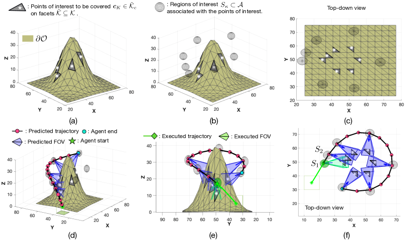
Figure 1: The figure shows an illustrative example of the stage-1 controller.

Finally, the stage-2 controller solves the optimization problem shown in (15) to robustly guide the agent inside $S_{\kappa}$ with probability at least $1-\epsilon$.

[h!]

$$~{}~{}\underset{\{\boldsymbol{u}\in\mathcal{U}\}}{\min}~{}\mathcal{J}^{0}=\sum_{t=1}^{T}||\boldsymbol{u}_{t-1}||_{2}^{2}$$ (15a)

subject to: $$\tau\in\{0,..,{T^{\prime}}-1\},n\in\{1,..,4\}$$

$$\boldsymbol{\mu}^{n}_{t+\tau+1|t}=A^{mom_{n}}_{t+\tau|t}\boldsymbol{\mu}^{n}_{t+\tau|t}+B^{mom_{n}}_{t+\tau|t}, \forall n,\tau$$ (15b)

$$\boldsymbol{\mu}^{n}_{t|t}=\boldsymbol{\mu}^{n}_{t-1|t}, \forall n,\tau$$ (15c)

$$\frac{4}{9}\frac{\mathbb{E}[(f^{\kappa}_{t+{T^{\prime}}|t})^{2}]-\mathbb{E}[f^{\kappa}_{t+{T^{\prime}}|t}]^{2}}{\mathbb{E}[f^{\kappa}_{t+{T^{\prime}}|t}]^{2}}\leq\epsilon,$$ (15d)

4 Evaluation

4.1 Simulation Setup

To demonstrate the proposed approach we have used the following simulation setup: the agent dynamics are given by (1) with horizontal and vertical velocities set as $u_{t}^{\nu}\in[0,10]~{}\text{m}/\text{s}$, and $u_{t}^{z}\in[-10,10]~{}\text{m}/\text{s}$ respectively. The yaw rate is given by $u_{t}^{\psi}\in[-\pi,\pi]~{}\text{rad}/\text{s}$, and the sampling interval is $\Delta_{t}=0.1$s. The disturbance $\boldsymbol{\omega}_{t}=[\omega^{\nu}_{t},\omega^{z}_{t},\omega^{\psi}_{t}]^{\top}$ is defined as follows: $\omega^{\nu}_{t}$ follows a Beta distribution with parameters $\alpha=1$, and $\beta=3$, $\omega^{z}_{t}$ follows a zero-mean Gaussian distribution $\mathcal{N}(0,0.3)~{}\text{m}/\text{s}$, and finally, $\omega^{\psi}_{t}$ follows a Uniform distribution in the range $[-0.1,0.1]~{}\text{rad}/\text{s}$. The agent camera FOV model parameters $(h_{f},w_{f},\ell_{f})$ are set to $(16,8,8)$m, and the gimbal rotation angles $\phi^{y}$ and $\phi^{z}$ take their values from the finite sets $\Phi^{y}=\{\frac{\pi}{8},\frac{\pi}{4},\frac{3\pi}{8},0,-\frac{\pi}{8},-\frac{\pi}{4},-\frac{3\pi}{8}\}~{}\text{rad}$, and $\Phi^{z}=\{\frac{\pi}{4},0,-\frac{\pi}{4}\}~{}\text{rad}$, respectively leading to $|\mathcal{M}|=21$ possible camera FOV configurations. Finally, we should mention that the stage-1 controller in (3) was implemented as a mixed integer quadratic program (MIQP), and solved using the Gurobi solver, whereas the stage-2 controller in (15) was solved using off-the-shelf non-linear optimization tools.

4.2 Results

An illustrative example of the proposed approach is shown in Fig. 1. Specifically, Fig. 1(a) shows the object of interest $O$ to be covered with its surface area $\partial O$ given by the function $q(x,y)=40\exp\left(-\left(\frac{(x-45)^{2}}{160}+\frac{(y-45)^{2}}{160}\right)\right)$, triangulated into a 3D mesh composed of $338$ triangular facets $K\in\mathcal{K}$. A subset $\tilde{\mathcal{K}}$ of those facets have been randomly sampled, and their centroids $\boldsymbol{c}_{K}\in\tilde{\mathcal{K}}_{c}$ have been marked for coverage. In total, $|\tilde{\mathcal{K}}_{c}|=7$ points of interest need to be covered as shown in Fig. 1(a). For each point of interest $\boldsymbol{c}_{K}\in\tilde{\mathcal{K}}_{c}$, we have associated a region of interest $S_{\kappa}$ ($\ell=12\text{m},s_{r}=3\text{m}$), where $\kappa$ is the index to the associated point $\boldsymbol{c}_{K}$ of facet $K$, also shown in Fig. 1(b)-(c).

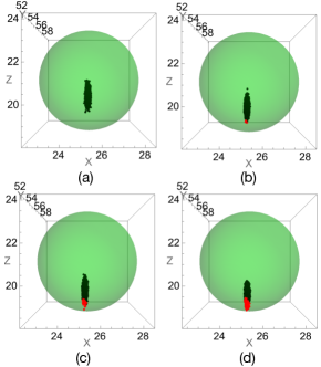
Figure 2: The figure illustrates a Monte-Carlo simulation of the agent’s state (i.e., position) at the end of the horizon obtained by the stage-2 controller for different confidence levels $\epsilon$. (a) $\epsilon=0.005$, (b) $\epsilon=0.0250$, (c) $\epsilon=0.05$, and (d) $\epsilon=0.1$.

Then, Fig. 1(d)-(f) shows the reference coverage plan generated by the model-predictive stage-1 controller discussed in Sec. 3.1, by optimizing (3a) with $w=10^{-3}$. In particular, Fig. 1(d) illustrates the agent’s trajectory inside a rolling planning horizon of length $T=14$ time-steps, generated according to the high-level dynamics shown in (3b) with $\Delta^{1}_{t}=1\text{s}$, and $|\boldsymbol{u}^{1}_{t}|\leq 10\text{m}/\text{s}$. In this experiment, we select FOV configurations from the set $\mathcal{M}$. As demonstrated in Fig. 1(d), the trajectory $\boldsymbol{x}^{1}_{1+\tau+1|1}$, for $\tau\in\{1,..,14\}$, is guided through the regions of interest, selecting FOV configurations that result in the coverage of the points of interest by optimizing (3a). Similarly, Fig. 1(e)-(f) displays the generated reference plan $\boldsymbol{x}^{1}_{6+\tau+1|6}$ for $\tau\in\{1,..,14\}$, with the executed coverage plan marked green.

As we have already discussed, at every time-step the stage-1 controller generates the coverage reference plan, and sends the region of interest to be visited next to the stage-2 controller.

Subsequently, the stage-2 controller aims to: robustly guide the agent inside the region of interest. This is demonstrated in next, Fig. 2 with a Monte-Carlo simulation of the output of stage-2 controller during the transition of the agent from $S_{1}$ to $S_{2}$, (as shown in Fig. 1(f)) over a planning horizon of $T^{\prime}=14$ time-steps, for different confidence levels $\epsilon$. The figure shows the agent’s position at the end of the planning horizon. Specifically, Fig. 2(a) shows 10000 samples of the agent’s final position for $\epsilon=0.005$. As shown, all samples of the agent’s position reside inside the region of interest indicated by the green sphere (i.e., $S_{2}$). Similarly, Fig. 2(b), Fig. 2(c), and Fig. 2(d) shows the same result for $\epsilon=0.0250$, $\epsilon=0.05$, and $\epsilon=0.1$ respectively. As shown in the figure, the red points indicate samples violating the constraints but always within the selected confidence level. In Fig. 2(b), 4 samples (out of 10000) reside outside the region of interest, well below the desired $\epsilon$ which is un upper bound of the violation probability. The same applies for Fig. 2(c) and Fig. 2(d) where 56 and 377 samples violate the constraints respectively.

5 Conclusion

We introduce a two-stage hierarchical fault-tolerant coverage controller for UAVs to cover 3D points of interest. The first stage formulates a hybrid optimal control problem, optimizing UAV mobility and camera control inputs for maximal coverage. The second stage employs mixed-trigonometric-polynomial moment propagation, to generate fault-tolerant coverage trajectories by accommodating non-Gaussian disturbances on the control inputs propagated through the system’s nonlinear dynamics. Future work will explore fault-tolerant camera control and fault-tolerant multi-agent coverage control.

References

• Bircher et al. (2018) Bircher, A., Kamel, M., Alexis, K., Oleynikova, H., and Siegwart, R. (2018). Receding horizon path planning for 3d exploration and surface inspection. Autonomous Robots, 42, 291–306.
• Cabreira et al. (2019) Cabreira, T.M., Brisolara, L.B., and Ferreira Jr, P.R. (2019). Survey on coverage path planning with unmanned aerial vehicles. Drones, 3(1), 4.
• Calafiore and Fagiano (2013) Calafiore, G.C. and Fagiano, L. (2013). Robust model predictive control via scenario optimization. IEEE Transactions on Automatic Control, 58(1), 219–224.
• Cannata and Sgorbissa (2011) Cannata, G. and Sgorbissa, A. (2011). A minimalist algorithm for multirobot continuous coverage. IEEE Transactions on Robotics, 27(2), 297–312.
• Choset (2000) Choset, H. (2000). Coverage of known spaces: The boustrophedon cellular decomposition. Autonomous Robots, 9(3), 247–253.
• Dai et al. (2019) Dai, S., Schaffert, S., Jasour, A., Hofmann, A., and Williams, B. (2019). Chance constrained motion planning for high-dimensional robots. In Proc. IEEE Int. Conf. on Robot. and Aut. (ICRA), 8805–8811.
• Galceran and Carreras (2013) Galceran, E. and Carreras, M. (2013). A survey on coverage path planning for robotics. Robotics and Autonomous Systems, 61(12), 1258–1276.
• Han et al. (2022) Han, W., Jasour, A., and Williams, B. (2022). Non-gaussian risk bounded trajectory optimization for stochastic nonlinear systems in uncertain environments. In Proc. IEEE International Conference on Robotics and Automation (ICRA), 11044–11050.
• Huang (2001) Huang, W.H. (2001). Optimal line-sweep-based decompositions for coverage algorithms. In Proceedings 2001 ICRA. IEEE International Conference on Robotics and Automation, volume 1, 27–32. IEEE.
• Janchiv et al. (2013) Janchiv, A., Batsaikhan, D., Kim, B., Lee, W.G., and Lee, S.G. (2013). Time-efficient and complete coverage path planning based on flow networks for multi-robots. International Journal of Control, Automation and Systems, 11(2), 369–376.
• Jasour et al. (2021) Jasour, A., Wang, A., and Williams, B.C. (2021). Moment-based exact uncertainty propagation through nonlinear stochastic autonomous systems. arXiv preprint arXiv:2101.12490 [eess.SY].
• Jiao et al. (2010) Jiao, Y.S., Wang, X.M., Chen, H., and Li, Y. (2010). Research on the coverage path planning of uavs for polygon areas. In 2010 5th IEEE Conference on Industrial Electronics and Applications, 1467–1472.
• Lew et al. (2020) Lew, T., Bonalli, R., and Pavone, M. (2020). Chance-constrained sequential convex programming for robust trajectory optimization. In Proc. IEEE European Control Conference (ECC), 1871–1878.
• Li et al. (2011) Li, Y., Chen, H., Er, M.J., and Wang, X. (2011). Coverage path planning for UAVs based on enhanced exact cellular decomposition method. Mechatronics, 21(5), 876–885.
• Mayne et al. (2005) Mayne, D.Q., Seron, M.M., and Raković, S. (2005). Robust model predictive control of constrained linear systems with bounded disturbances. Automatica, 41(2), 219–224.
• Mercadier and Strobel (2021) Mercadier, M. and Strobel, F. (2021). A one-sided vysochanskii-petunin inequality with financial applications. European Journal of Operational Research, 295(1), 374–377.
• Papaioannou et al. (2023) Papaioannou, S., Kolios, P., and Ellinas, G. (2023). Distributed estimation and control for jamming an aerial target with multiple agents. IEEE Transactions on Mobile Computing, 22(12), 7203–7217.
• Papaioannou et al. (2022) Papaioannou, S., Kolios, P., Theocharides, T., Panayiotou, C.G., and Polycarpou, M.M. (2022). Integrated ray-tracing and coverage planning control using reinforcement learning. In 2022 IEEE 61st Conference on Decision and Control (CDC), 7200–7207. IEEE.
• Phung et al. (2017) Phung, M.D., Quach, C.H., Dinh, T.H., and Ha, Q. (2017). Enhanced discrete particle swarm optimization path planning for uav vision-based surface inspection. Automation in Construction, 81, 25–33.
• Summers (2018) Summers, T. (2018). Distributionally robust sampling-based motion planning under uncertainty. In Proc. IEEE/RSJ International Conference on Intelligent Robots and Systems (IROS), 6518–6523.
• Taubin (2011) Taubin, G. (2011). 3d rotations. IEEE Computer Graphics and Applications, 31(6), 84–89.
• Vitale et al. (2022) Vitale, C., Papaioannou, S., Kolios, P., and Ellinas, G. (2022). Autonomous 4D trajectory planning for dynamic and flexible air traffic management. Journal of Intelligent & Robotic Systems, 106(1), 11.
• Xie et al. (2020) Xie, J., Garcia Carrillo, L.R., and Jin, L. (2020). Path planning for uav to cover multiple separated convex polygonal regions. IEEE Access, 8, 51770–51785.
• Xu et al. (2014) Xu, A., Viriyasuthee, C., and Rekleitis, I. (2014). Efficient complete coverage of a known arbitrary environment with applications to aerial operations. Autonomous Robots, 36(4), 365–381.