With Andrzej Lasota there and back again
Abstract.
The paper below is a written version of the 17th Andrzej Lasota Lecture presented on January 12th, 2024 in Katowice. During the lecture we tried to show the impact of Andrzej Lasota’s results on the author’s research concerning various fields of mathematics, including chaos and ergodicity of dynamical systems, Markov operators and semigroups and partial differential equations.
Key words and phrases:
chaos, invariant measure, partial differential equation, Markov operator, semigroup of operators, asymptotic stability, piecewise deterministic Markov process, application to biological models2020 Mathematics Subject Classification:
35F25; 37A05; 37L40; 47D06; 60J76; 92D251. Introduction
Let us start with a brief introduction of Professor Andrzej Lasota (1932–2006). He studied physics and mathematics at Jagiellonian University (1951–1955). From 1955–1975 he worked at Jagiellonian University, where he was the Dean of the Faculty of MPCh (1972–1975).
He then moved to Katowice at the University of Silesia, where he worked until his death with a short break in the years of 1986–1988 spent at Maria Curie-Skłodowska University in Lublin. During that time he had also part-time positions at Jagiellonian University (1975–2005) and Institute of Mathematics Polish Academy of Sciences (1995–2006).
His research interests concerned the following areas of mathematics:
-
(1)
differential equations,
-
(2)
dynamical systems: chaos, ergodicity and fractal theory,
-
(3)
Markov operators,
-
(4)
applications of mathematics to biology, physics and technology.
I met Professor Lasota at his lecture on the theory of differential equations in 1977, and after the exam, I began my research under his supervision. This was a period when he conducted very intensive research dealing with a variety of issues in pure and applied mathematics collaborating with well-known scholars, including J.A. Yorke – American mathematician co-founder of chaos theory and M.C. Mackey – Canadian biomathematician (see Fig. 1). This gave me the opportunity to learn about top scientific issues and join in this research.

During the lecture, I tried to show the impact of Andrew Lasota’s results on my research. I will focus on a few selected topics, mainly on chaos theory for partial differential equations and asymptotics of Markov operators and semigroups and their applications in biology.
2. Chaos and ergodicity of dynamical systems
2.1. General remarks
Since the issues of chaos and ergodicity will occur at various points in the lecture, we will now collect the necessary definition and basic results. A more extensive introduction to these issues is presented in the survey papers [33, 36].
Let be a metric space. A semiflow on is a collection of transformation , for , such that
-
(a)
, for ,
-
(b)
, defined as , is a continuous function of .
The set is called an orbit of the point .
For example if is a Lipschitz function then the problem
has unique solution and defines a semiflow on .
If is a continuous map, then the sequence of its iterates creates a discrete time semiflow. Discrete and continuous time semiflows belong to a broader class called dynamical systems. In a dynamical system, instead of the continuity condition (b), for example, we can assume the measurability of a function .
When can we say that a dynamical system is chaotic? General answer is that it has a simple and deterministic description, but it behavies in a complicated and random way. Random means here that the semiflow has unpredictable behaviour. The semiflow is very sensitive on small perturbations of initial data and looks like a system with a stochastic noise.
Almost all specialists are willing to accept this not too precise definition. But, in fact, there are hundreds of definitions of chaos. Generally we have three different approaches to chaos.
1. Macroscopic approach: the existence of global attractors with complicated structure (strange attractors).
2. Microscopic approach: the existence of trajectories, which are unstable, turbulent or dense in the phase space; topologically mixing.
3. Stochastic approach: the existence of invariant measures having strong ergodic and analytic properties.
It should be noted that our “classification” of chaotic behaviour is completely arbitrary, but it could help non-specialists what kind of problems are studied in the theory of chaos. In the lecture, I will focus on the connections between the second and third approaches to justify that the methods of ergodic theory allow us to obtain quite strong chaotic properties.
2.2. Microscopic approach
In this approach we have several different definitions of chaos. A flow is chaotic in the sense of Auslander–Yorke [1] if
-
(a)
there exists a dense trajectory,
-
(b)
each trajectory is unstable.
Let us mention that a semiflow on some topological vector space having a dense orbit is said to be hypercyclic [7], which in the case when is a Baire space it is equivalent to the flow being topologically transitive. We consider a strong version of unstability, which is also called sensitive dependence on initial conditions: there exists a constant such that for each point and for each there exist a point and such that . Here denotes the open ball in with centre and radius .
A little stronger definition of chaos was given by Devaney [6]:
-
(a’)
there exists a dense trajectory,
-
(b’)
the set of periodic points is dense in .
One can check that from (a’) and (b’) it follows that each trajectory is unstable.
A semiflow is topologically mixing if for any two non-empty open sets , of there exists such that for . The topological mixing is a strong chaotic property of a transformation and implies chaos in the sense of Auslander–Yorke and sensitive dependence on initial conditions.
One of the chaotic properties of a semiflow is turbulence. A trajectory of the point is turbulent in the sense of Lasota–Yorke [13], if its closure is a compact set and does not contain periodic points.
Theorem 1.
Let be a semiflow. If for some nonempty, compact, and disjoint sets and we have
| (1) |
then there exists a turbulent orbit in the sense of Lasota–Yorke.
2.3. Stochastic approach
We recall some necessary definitions.
By a measure on we mean any probability measure defined on the -algebra of Borel subsets of . By we denote the topological support of the measure .
A measure is called invariant under a semiflow , if for each and each Borel subset . Here . We will denote a semiflow with an invariant measure by .
The semiflow is called ergodic if for each -integrable function we have
| (2) |
If we substitute in equation (2), then the left-hand side of (2) is the mean time of visiting the set and the right-hand side of (2) is .
A semiflow is called mixing if
| (3) |
for all . If and then condition (3) can be written in the following way
which means that the trajectory of almost all points enters a set with asymptotic probability .
The semiflow is exact if for each measurable set with we have
| (4) |
We have: exactness mixing ergodicity.
We now show how ergodic properties of a semiflow imply its chaotic behaviour.
Proposition 1.
Let be a separable metric space and be a probability Borel measure on such that . If a semiflow is ergodic, then the orbit of –a.e. point is dense in . If a semiflow is mixing, then the semiflow is topologically mixing, in particular has the property of sensitive dependence on initial conditions.
Sometimes the combination of the methods of ergodic theory and dynamical systems allows us to obtain stronger properties of the considered systems. We combine the following well known Krylov–Bogoliubov theorem with condition (1).
Theorem 2.
Let be a semiflow on a compact metric space. Then there exists a probability Borel measure invariant and ergodic with respect to .
This theorem is a nice general result, but if the semiflow has a periodic point , this result is trivial, because we find an invariant ergodic measure supported on the orbit of . To formulate a stronger version of Theorem 2 we need the following definition. A measure is said to be continuous if , where Per is the set of all periodic points of the semiflow .
Theorem 3.
Let be a semiflow on a compact metric space. If there are nonempty, compact, and disjoint sets and satisfying condition , then there exists a continuous probability Borel measure invariant and ergodic with respect to .
Proof.
3. Frobenius–Perron operator and ergodic properties
3.1. Introduction
Ergodic properties of semiflows can be successfully investigated using methods of operator theory [10]. We now introduce the notion of Frobenius–Perron operator and show how ergodic properties of flows can be expressed in the language of Frobenius–Perron operators.
Let be a -finite measure space. A measurable map is called non-singular if it satisfies the following condition
| (5) |
Let and let be a nonsingular map of . An operator which satisfies the following condition
| (6) |
is called the Frobenius–Perron operator for the transformation . The operator is linear, positive (if then ) and preserves the integral (). The adjoint of the Frobenius–Perron operator is given by .
Denote by the set of all densities with respect to , i.e. functions such that and . Let be a nonsingular transformation and let . Then the measure for , is invariant with respect to if and only if .
Now we consider a family of transformations , where or . If the map is measurable and each transformation is nonsingular, then we denote by the Frobenius–Perron operator corresponding to . Then the quadruple is a measure-preserving dynamical system if and only if for all . We collect the relations between ergodic properties of dynamical systems and the behavior of the Frobenius–Perron operators in Table 1.
| invariant | for all |
|---|---|
| ergodic | is a unique fixed point in of all |
| mixing | w- for every |
| exact | for every |
We recall that the weak limit w- is a function such that for every we have
3.2. Lasota–Yorke lower function theorem
A. Lasota and J.A. Yorke have developed tools to study the convergence of Frobenius–Perron operators and there applications to expanding maps [12]. One of such tools is the lower function theorem [14]. This theorem can be applied to a broader class of operators called Markov or stochastic operators, so we will start with a definition of them.
Let be a -finite measure space. A linear operator is called a Markov (or stochastic) operator if .
The family of Markov operators is called a stochastic semigroup if it satisfies the following conditions:
-
(a)
, i.e., ,
-
(b)
,
-
(c)
for each the function is continuous.
We also consider a discrete time stochastic semigroup defined as the iterates of a Markov operator.
Markov operators appear in ergodic theory of dynamical systems and iterated function systems. They also describe the evolution of Markov chains. Stochastic semigroups describe the evolution of densities of distributions of Markov processes like diffusion processes, piecewise deterministic processes and hybrid stochastic processes.
Consider a stochastic semigroup . A density is called invariant if for each . The stochastic semigroup is called asymptotically stable if there is an invariant density such that
A function , and , is called a lower function for a stochastic semigroup if
for each density . This condition can be equivalently written as:
Observe that if the semigroup is asymptotically stable then its invariant density is a lower function for it. Lasota and Yorke [14] proved the following converse result.
Theorem 4.
If there exists a lower function for a stochastic semigroup then this semigroup is asymptotically stable.
3.3. An generalization of the lower function theorem
G. Pianigiani and J.A. Yorke [20] considered the following problem. Let be a compact subset of and let be a piecewise expanding map. We consider the sequence of iterates of points from as long as they still remain in the set . If , then we lose the orbit of . We consider the following problem. If the initial distribution of points is given by a probability measure , what is the conditional probability that given that are in ? Such a problem can be called a discrete time billiard with holes, because we can treat as a table with holes and the transformation describes the motion of a ball which can fall through some hole.
We can define the Frobenius–Perron operator for the map . The operator is positive, but since the set is not containing in , the operator does not preserve the integral. If has a density , then has density and is the fraction of points such that the sequence lies in the set .
Since Theorem 4 was useful to study asymptotic stability of Frobenius–Perron operators of piecewise expanding maps , we hoped that it is possible to find a version of this theorem which can be successfully applied to billiards with holes. The problem was solved in [30], but instead of operators on the space we consider operators on . The result is the following.
Theorem 5.
Let be a compact Hausdorff space, be a positive operator on , be a dense subset of }, and . We assume that for each there exists a constant such that
We also assume that for some , the sequence has a weakly convergent subsequence. Then there exist a probability measure , , and a function such that , and
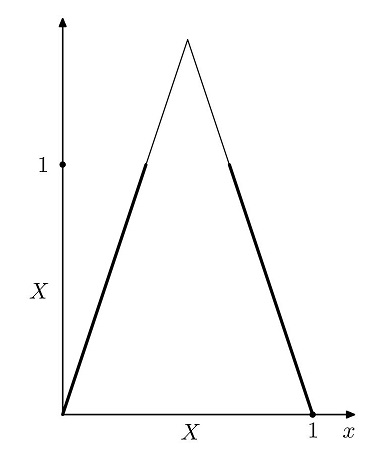
Consider the following example: is given by , (see Fig. 2). Then
In this example we have
and the support of the measure is similar to the Cantor’s set.
A continuous version of Theorem 5 was proved in [11] and applied to study the movement of a point on a circle with random jumps. Nowadays, such a movement is called a piecewise deterministic Markov process, although at the time we did not know this name. We also applied this theorem to some partial differential equations with integral perturbation. Methods presenting in papers [11, 30] are also used in the paper with M.C. Mackey [17] to study the asymptotic behaviour of non-homogeneous age dependent cellular populations. A non-autonomous version of Theorem 5 was proved by A. Lasota and J.A. Yorke [15].
4. Asymptotic behaviour of stochastic semigroups
4.1. Partially integral stochastic semigroups
We will now present methods for studying the asymptotics of stochastic semigroups based on an idea reminiscent of the use of the lower function. It involves estimating a semigroup from below using an integral operator.
A Markov semigroup is called partially integral if there exist and a measurable function , such that
and
Using the theory of Harris operators one can prove many interesting results concerning partially integral stochastic (and substochastic) semigroups.
The basic results have been published in the paper [32], but we will limit ourselves to a few selected later results. In [21] was proved the following result.
Theorem 6.
If a continuous time partially integral stochastic semigroup has a unique invariant density and , then it is asymptotically stable.
4.2. Asymptotic decomposition of a stochastic semigroups
The main problem with applying Theorem 6 is that often it is not easy to find an invariant density. To get around this difficulty, in [22] was devised a method of studying of stochastic semigroups via their asymptotic decomposition. To present this method, from now on we assume additionally that is a separable metric space and is the -algebra of Borel subsets of . We consider stochastic semigroups which satisfy the following condition:
(K) for every there exist an , a , and a measurable function such that and
| (7) |
where . It is clear that stochastic semigroups satisfying condition (K) are partially integral. Now we present the main theorem of [22].
Theorem 7.
Let be a continuous time stochastic semigroup which satisfies (K). Then there exist a countable (possible empty) set , a family of invariant densities with disjoint supports , and a family of positive linear functionals defined on such that
-
(i)
for every and for every we have
(8) -
(ii)
if , then for every and for every compact set we have
(9)
We note that not only the sets , , are disjoint but also their closures are disjoint, which means that the measures have disjoint topological supports [23].
In order to formulate a corollary of Theorem 7, we need an auxiliary notion. A stochastic semigroup is called sweeping from a set if for every
Corollary 1.
Assume that a stochastic semigroup satisfies condition (K) and has no invariant densities. Then is sweeping from compact sets.
This result also holds for discrete time stochastic semigroups.
Theorem 7 allows us also to find conditions guaranteeing that a stochastic semigroup satisfies the Foguel alternative, i.e. it is asymptotically stable or sweeping from all compact sets. An advantage of the formulation of some results in the form of the Foguel alternative is that in order to show asymptotic stability we do not need to prove the existence of an invariant density. It is enough to check that the semigroup is not sweeping from compact sets then, automatically, the semigroup is asymptotically stable. A more comprehensive introduction to the subject of convergence and asymptotic behaviour of semigroups of operators can be found in [3].
4.3. Applications to piecewise deterministic Markov processes
Theorems from Section 4.2 are very useful in the study of stochastic semigroups generated by Markov processes. In the case of diffusion processes, the semigroups describing the evolution of the density of distributions of the process are integral and have continuous and positive kernels. Hence, Theorem 7 can be applied without additional conditions and we immediately obtain the Foguel alternative. Theorem 7 is satisfied by a semigroup induced by any Markov chains because the space is discrete. This semigroup satisfies the Foguel alternative if the chain is irreducible. It turns out that the theorem can also be applied to piecewise deterministic Markov processes (PDMPs). We will now give a definition of a PDMP and explain why such processes lead to partially integral semigroups.
According to a non-rigorous definition by Davis [5], the class of PDMPs is a general family of stochastic models covering virtually all non-diffusion applications. A more formal definition of a PDMP is the following. A continuous time (homogeneous) Markov process is a PDMP if there is an increasing sequence of random times , called jumps, such that the sample paths of are defined in a deterministic way in each interval .
We consider three types of jumps:
-
a)
the process can jump to a new point,
-
b)
at the moment of jump it changes the dynamics which defines its trajectories,
-
c)
changes the dynamics when it hits some surface (a stochastic billiard).
The induced semigroup by a PDMP is generally not integral, but because the jumps are at random moments there is a “blurring” of distributions. For example, from a distribution concentrated at a point we get an absolutely continuous distribution with respect to the Lebesgue measure, which leads to a partially integral semigroup.
Flows with jumps (see Fig. 3) are used in models of population growth with disasters, immune systems [26, 27] and cell cycle models [25, 28].
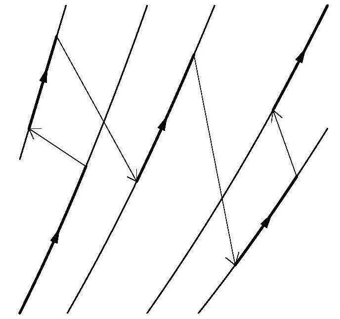
Processes with switching dynamics (see Fig. 4) describe the action of several flows with random switching between them. They are used as models of gene regulatory networks [2, 39]. Depending on the state of activity of the genes occurring in the network, such a model is described by different systems of differential equations. A change in gene activity switches the system.
We also consider processes in which a change in dynamics or a jump in phase space occurs when the process reaches the boundary of the domain or some fixed subset of the phase space. An example of such a process is a stochastic billiard [4, 16, 19]. Similar properties have models of cell cycle and neuron activity [24]. A more comprehensive introduction to PDMPs and there applications can be found in [37, 40].
5. Invariant measures for partial differential equations
5.1. Lasota example
It is hardly known that solutions of simple linear partial differential equations behave in a chaotic way or have interesting ergodic properties. Consider the following equation with the initial condition:
| (10) |
This equation can served as a very simple model of the dynamics of cell maturation. Here is the cell maturity, is the maturation rate. If is the rate of population growth, then .
If the space is finite dimensional, then ergodic properties of semiflows can be successfully investigated by means of Frobenius–Perron operators. But this method is rather difficult to apply in the infinite dimensional space . A. Lasota [8] proposed to apply Theorem 3 to this flow and he proved that if , then there is a continuous ergodic measure on invariant with respect to .
The disadvantage of this method is that the constructed measure has a relatively small support and it is not mixing, and thus we cannot use it to prove the chaotic properties discussed in Sec. 2.3. In particular we are not able to prove that the semiflow has a dense orbit and has the property of sensitive dependence on initial conditions.
Looking for a method to construct invariant measures that have the desired properties, I noticed that it would be more convenient to use a method based on isomorphism of the flow with a translation semiflow and using measure introduced by some stationary process. We will present this method in the next section, but now we only mention that an invariant mixing measure with can be given by the formula , where and is the standard Wiener process. Since problem (10) describes the evolution of distribution of maturity in a cellular population one can prefer to consider the semiflow restricted to the set . In this case the invariant measure on can be induced by the process .
5.2. General approach
Now we consider semiflow generated by the equation of the form
| (11) |
We assume that and are -functions and , for , , , for . Let
This flow was studied in [29, 31] and, among other things, it was proved the following theorem.
Theorem 8.
There exists a probability measure such that:
(a) is invariant with respect to ,
(b) is exact,
(c) .
Draft of the proof.
Let and
let be the left-side shift on the space
defined by .
1. The semiflows
and
are isomorphic, i.e.
the map given by is
a homeomorphism of onto
and
| (12) |
2. Let , , be the Wiener process and for . Then is a stationary Gaussian process with continuous trajectories. Let
The measure is invariant under
and .
Thus the measure is invariant under .
3. Exactness of follows from
the Blumenthal’s zero-one law for the Wiener process; from
the definition of the measure ; and from an equivalent definition of exactness.
4. Positivity of on open sets can be obtained from
the following property of Wiener process:
for continuous functions and . ∎
5.3. Other chaotic models
The method of constructing invariant measures presented in Section 5.2 can be used for semiflows generated by other partial differential equations, although the proofs are no longer as easy as for Eq. (11). We will briefly present other equations studied using this method.
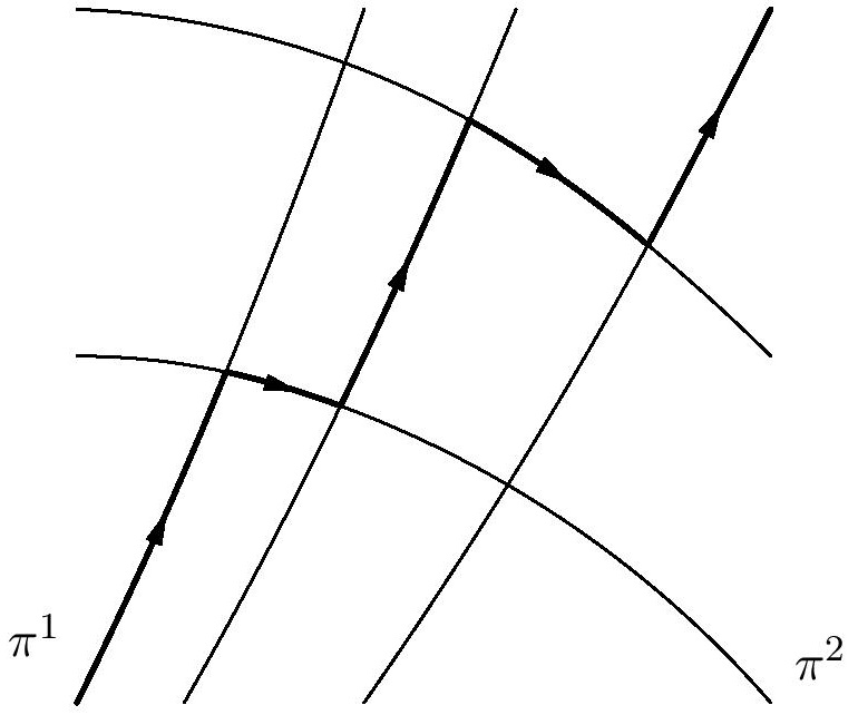
We consider a population of stem cells. These cells live in the bone marrow and they are precursors of any blood cells. They are subjects of two biological processes: maturation and division. Stem cells can be at different levels of morphological development called maturity. The maturity of a cell differs from its age, because we assume that a newly born cell is in the same morphological state as its mother at the point of division. We assume that maturity is a real number . The function describes the density distribution function of cells with respect to their maturity. The maturity grows according to the equation . When one cell reaches the maturity it leaves the bone marrow, then one of cells from the bone marrow splits. This cell is chosen randomly according to the distribution given by the density . It follows from the assumptions that a newly born cell has the same maturity as its mother cell and each cell can divide with the same probability (see Fig. 5).
There is an exterior regulatory system in which the production of erythrocytes is stimulated by the hormone erythropoietin and the system tries to keep the number of erythrocytes on a constant level. We have not added this external regulatory system, thus we consider a pathological case when the exterior regulatory system does not work. The model is described by a nonlinear semiflow induced by the problem
| (13) |
The semiflow is defined on the space of densities. In the paper [34] it was shown that the semiflow generated by the initial problem (13) posses an invariant measure which is mixing and supported on the whole set of all densities.
The second example is the Bell and Anderson model of size structured cellular population given by the equation
| (14) |
where and we put if . In [35] it was shown that if , then there exists a mixing invariant measure supported on the whole space.
The next example is -dimensional model considered in the paper [38]:
In construction of invariant measure we use Lévy -parameter Brownian motion, which is a Gaussian random field, and we show that the semiflow is isomorphic with a translation flow along the radii.
The last example is the heat equation:
| (15) |
with the boundary and initial conditions
| (16) |
Here we construct an invariant mixing measure supported on the phase space .
6. Remarks and Conclusions
6.1. Other mathematical research inspired by biology
I devoted the lecture mainly to presenting some mathematical issues without going too far into discussing their applications to biological models. Finally, I would like to show with the example of A. Lasota and my experience, that the study of biological issues can be inspiring for the development of mathematical methods. 1. Cell cycle modeling has influenced the development of the theory of Markov operators and the study of their asymptotic properties.
2. Structural population models lead to the development of the theory of transport equations, other than those found in physics, and the theory of semigroup operators.
3. The study of population models involves non-trivial nonlinear and non-local partial differential equations with delays [18]. Studying the behavior of solutions to such equations is quite a challenge for mathematicians.
4. Biologists are increasingly using individual-based models, also known as agent-based models. Individual-based models describe a population as a collection of different organisms whose local interactions determine the behaviour of the entire population. The individual description is convenient for computer simulations and the determination of various model parameters, and appropriate limit passages lead to interesting transport equations. For example, the phenotypic model studied in the paper [41] after an appropriate limit passage leads to a transport equation, including the Tjon-Wu equation of the energy distribution of particles in the Boltzmann equation, which was studied by A. Lasota [9].
6.2. To take home
1. Markov operators and semigroups can be used to describe and prove ergodic and chaotic properties of dynamical systems.
2. Markov semigroups describe the evolutions of densities of Markov processes: diffusion processes, piecewise deterministic Markov processes, stochastic hybrid systems (diffusions with jumps).
3. The chaotic properties of dynamical systems generated by partial differential equations can be successfully studied using stochastic processes.
4. Modern biology boldly reaches for mathematical models, and virtually every part of mathematics can be useful in modeling. Due to the random nature of biological phenomena, stochastics plays a major role in this regard.
5. We will conclude with a quote from Sir Rory Collins head of clinical research at Oxford University: “If you want a career in medicine these days you’re better off studying mathematics or computing than biology.”
References
- [1] J. Auslander and J.A. Yorke, Interval maps, factors of maps and chaos, Tôhoku Math. J. II. Ser. 32 (1980), 177–188.
- [2] A. Bobrowski, T. Lipniacki, K. Pichór, and R. Rudnicki, Asymptotic behavior of distributions of mRNA and protein levels in a model of stochastic gene expression, J. Math. Anal. Appl. 333 (2007), 753–769.
- [3] A. Bobrowski and R. Rudnicki, On convergence and asymptotic behaviour of semigroups of operators, Phil. Trans. R. Soc. A. 378 (2020), 20190613 (18 pages).
- [4] F. Comets, S. Popov, G. M. Schütz, and M. Vachkovskaia, Billiards in a general domain with random reflections, Arch. Ration. Mech. Anal. 191 (2009), 497–537.
- [5] M.H.A. Davis, Piecewise-deterministic Markov processes: a general class of nondiffusion stochastic models, J. Roy. Statist. Soc. Ser. B 46 (1984), 353–388.
- [6] R.L. Devaney, An Introduction to Chaotic Dynamical Systems, 2nd edn. Addison-Wesley Studies in Nonlinearity, Addison-Wesley Publishing Company, Redwood City, CA, 1989.
- [7] H.M. Hilden and L.J. Wallen, Some cyclic and non-cyclic vectors of certain operators, Indiana Univ. Math. J., 23 (1974), 557–565.
- [8] A. Lasota, Invariant measures and a linear model of turbulence, Rend. Sem. Mat. Univ. Padova, 61 (1979), 40–48.
- [9] A. Lasota, Asymptotic stability of some nonlinear Boltzmann-type equations, J. Math. Anal. Appl. 268 (2002), 291–309.
- [10] A. Lasota and M.C. Mackey, Chaos, Fractals and Noise. Stochastic Aspects of Dynamics, Springer Applied Mathematical Sciences 97, New York, 1994.
- [11] A. Lasota and R. Rudnicki, Asymptotic behaviour of semigroups of positive operators on , Bull. Polish Acad. Sci. Math. 36 (1988), 151–159.
- [12] A. Lasota and J. Yorke, On the existence of invariant measures for piecewise monotonic transformations, Trans. Amer. Math. Soc. 186 (1973), 481–488.
- [13] A. Lasota and J. Yorke, On the existence of invariant measures for transformations with strictly turbulent trajectories, Bull. Polish Acad. Sci. Math. 25 (1977), 233–238.
- [14] A. Lasota and J. Yorke, Exact dynamical systems and the Frobenius–Perron operator, Trans. Amer. Math. Soc. 273 (1982), 375–384.
- [15] A. Lasota and J. Yorke, When the long time behavior is independent of the initial density, SIAM J. Math. Anal. 27 (1996), 221–240.
- [16] B. Lods, M. Mokhtar-Kharroubi, and R. Rudnicki, Invariant density and time asymptotics for collisionless kinetic equations with partly diffuse boundary operators, Ann. I. H. Poincaré - AN 37 (2020), 877–923.
- [17] M.C. Mackey and R. Rudnicki, Asymptotic similarity and Malthusian growth in autonomous and nonautonomous populations, J. Math. Anal. Appl. 187 (1994), 548–566.
- [18] M.C. Mackey and R. Rudnicki, A new criterion for global stability of cell simultaneous cell replication and maturation processes, J. Math. Biol. 38 (1999), 195–219.
- [19] M. Mokhtar-Kharroubi and R. Rudnicki, On asymptotic stability and sweeping of collisionless kinetic equations, Acta Appl. Math. 147 (2017), 19–38.
- [20] G. Pianigiani and J.A. Yorke, Expanding maps on sets which are almost invariant: decay and chaos, Trans. Amer. Math. Soc. 252 (1979), 351–366.
- [21] K. Pichór and R. Rudnicki, Continuous Markov semigroups and stability of transport equations, J. Math. Anal. Appl. 249 (2000), 668–685.
- [22] K. Pichór and R. Rudnicki, Asymptotic decomposition of substochastic operators and semigroups, J. Math. Anal. Appl. 436 (2016), 305–321.
- [23] K. Pichór and R. Rudnicki, Asymptotic decomposition of substochastic semigroups and applications, Stoch. Dyn. 18 (2018), 1850001.
- [24] K. Pichór and R. Rudnicki, Stability of stochastic semigroups and applications to Stein’s neuronal model, Discrete Contin. Dyn. Syst. Ser. B 23 (2018), 377–385.
- [25] K. Pichór and R. Rudnicki, Applications of stochastic semigroups to cell cycle models, Discrete Contin. Dyn. Syst. Ser. B 24 (2019), 2365–2381.
- [26] K. Pichór and R. Rudnicki, Dynamics of antibody levels: asymptotic properties, Math. Method Appl. Sci. 43 (2020), 10490–10499.
- [27] K. Pichór and R. Rudnicki, Asymptotic properties of a general model of immune status, SIAM J. Appl. Math. 83 (2023), 172–193.
- [28] K. Pichór and R. Rudnicki, Cell cycle length and long-time behavior of an age-size model, Math. Meth. Appl. Sci. 45 (2022), 5797–5820.
- [29] R. Rudnicki, Invariant measures for the flow of a first-order partial differential equation, Ergod. Theory Dyn. Syst. 8 (1985), 437–443.
- [30] R. Rudnicki, Asymptotic properties of the iterates of positive operators on C(X), Bull. Acad. Pol. Sci. Math. 34 (1986), 181–188.
- [31] R. Rudnicki, Strong ergodic properties of a first-order partial differential equation, J. Math. Anal. Appl. 133 (1988), 14–26.
- [32] R. Rudnicki, On asymptotic stability and sweeping for Markov operators, Bull. Acad. Pol. Sci. Math. 43 (1995), 245–262.
- [33] R. Rudnicki, Chaos for some infinite-dimensional dynamical systems, Math. Meth. Appl. Sci. 27 (2004), 723–738.
- [34] R. Rudnicki, Chaoticity of the blood cell production system, Chaos 19 (2009), 043112.
- [35] R. Rudnicki, Chaoticity and invariant measures for a cell population model, J. Math. Anal. Appl. 393 (2012), 151–165.
- [36] R. Rudnicki, An ergodic theory approach to chaos, Discrete Contin. Dyn. Syst. Ser. A 35 (2015), 757–770.
- [37] R. Rudnicki, Models and Methods Mathematical Biology. Part II: Probabilistic Models, (in Polish), Ksiȩgozbiór Matematyczny 4, IMPAN, Warszawa 2022. (Modele i Metody Biologii Matematycznej, Czȩść II: Modele probabilistyczne).
- [38] R. Rudnicki, Ergodic properties of a semilinear partial differential equation, J. Differ. Equ. 372 (2023), 235–253.
- [39] R. Rudnicki and A. Tomski, On a stochastic gene expression with pre-mRNA, mRNA and protein contribution, J. Theor. Biol. 387 (2015), 54–67.
- [40] R. Rudnicki and M. Tyran-Kamińska, Piecewise Deterministic Processes in Biological Models, Springer Briefs in Applied Sciences and Technology, Mathematical Methods, Springer, Cham, Switzerland, 2017.
- [41] R. Rudnicki, P. Zwoleński, Model of phenotypic evolution in hermaphroditic populations, J. Math. Biol. 70 (2015), 1295–1321.