Fabry-Perot superconducting diode
Abstract
Superconducting diode effects (SDEs) occur in systems with asymmetric critical supercurrents yielding dissipationless flow in one direction , while dissipative transport in the opposite direction . Here we investigate the SDE in a phase-biased Josephson junction with a double-barrier resonant-tunneling InAs nanowire nested between proximitized InAs/Al leads with finite momentum Cooper pairing. Within the Bogoliubov-de Gennes (BdG) approach, we obtain the exact BCS ground state energy and from the current-phase relation . The SDE arises from the accrued Andreev phase shifts leading to asymmetric BdG spectra for . Remarkably, the diode efficiency shows multiple Fabry-Perot resonances at the double-barrier Andreev bound states as the well depth is varied. Our also features sign reversals for increasing and high sensitiveness to fermion-parity transitions. The latter enables switchings over narrow phase windows, i.e., , possibly relevant for future superconducting electronics.
I Introduction
Nonreciprocity in superconducting materials [1, 2, 3, 4, 5, 6, 7, 8, 9, 10, 11, 2, 12, 13, 14, 15, 16, 17, 18, 19, 20, 21] is currently a subject of particular interest. It refers to the asymmetry between the forward and reverse critical supercurrents such that . This has been observed in superconducting films [1, 2, 3], Josephson junctions [4, 5, 6, 7, 8], superconductor/ferromagnet multilayers [12, 13], as well as twisted trilayer graphene [9, 10]. Currents in the range , assuming , flow dissipationlessly in one direction (zero resistance), but dissipatively in the opposite direction (non-zero resistance). This is the superconducting diode effect (SDE) [14, 15, 16, 17, 18, 19, 20], conceptually similar to the p-n junction semiconducting diode.
A non-zero SDE generally requires breaking both time-reversal and spatial inversion symmetries [15, 17]. Time-reversal breaking can be achieved via, e.g., exchange fields which displace the Fermi surfaces in a spin-resolved fashion, thus making the Cooper pairs acquire a finite center-of-mass momentum [22, 23, 24, 25, 26, 27, 28]. Inversion asymmetry allows for a non-zero spin-orbit coupling and can result in a Fulde-Ferrell type phase-modulated pairing potential [29, 30, 31, 32]. The momentum can be controlled, e.g., by an external in-plane magnetic field and the spin-orbit interaction, which combined can change the Fermi surface [33, 34, 35, 36, 37, 38, 39, 40], by externally injecting currents [41, 42, 43] into the system and via the intrinsic screening supercurrents through the Meissner effect [11, 44]. Bulk superconductors and Josephson junctions alike can exhibit SDE. As we show next, superconductor-semiconductor hybrids enable proximity superconductivity in a semiconducting matrix, thus providing a unique setting to exploit SDE.
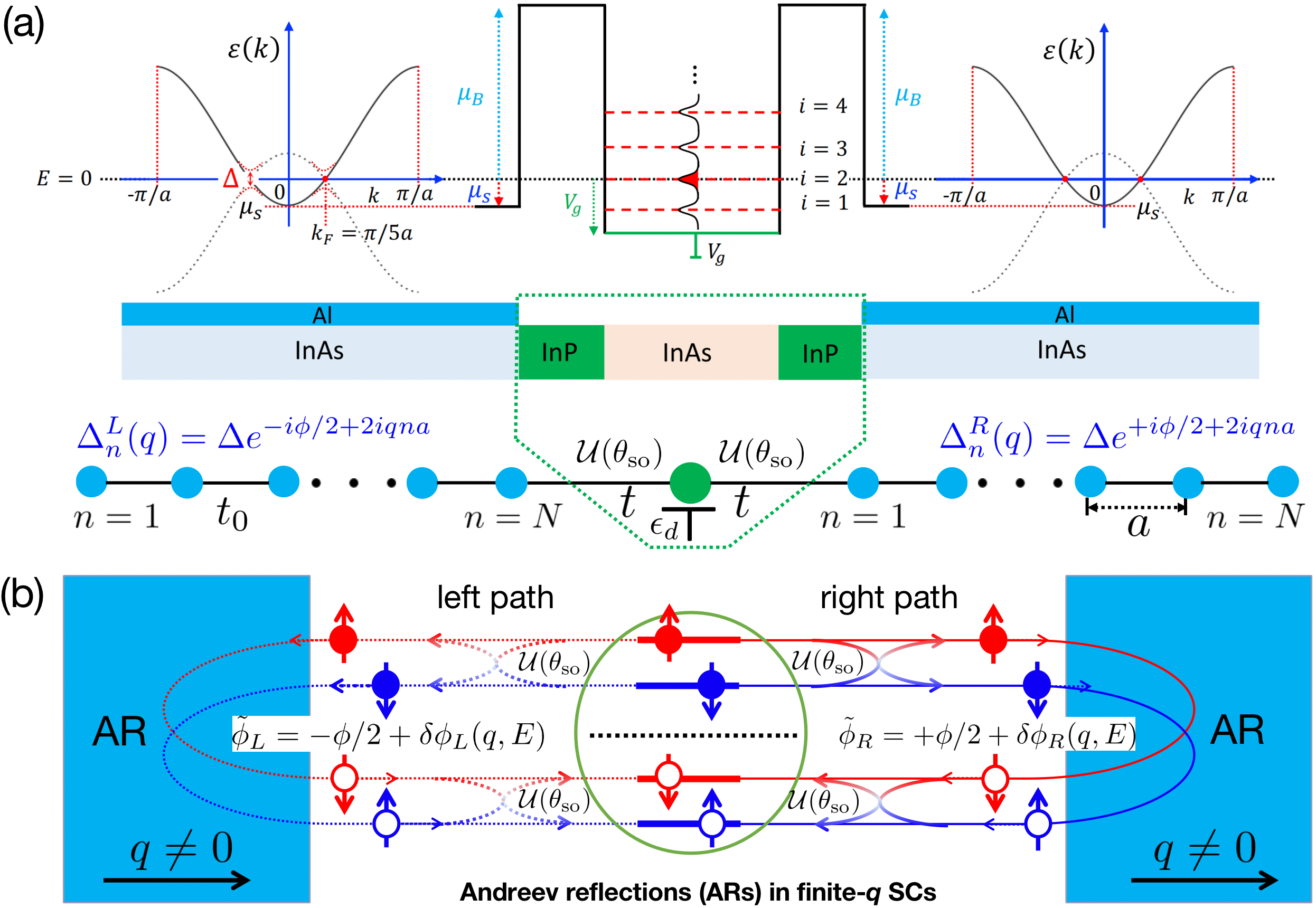
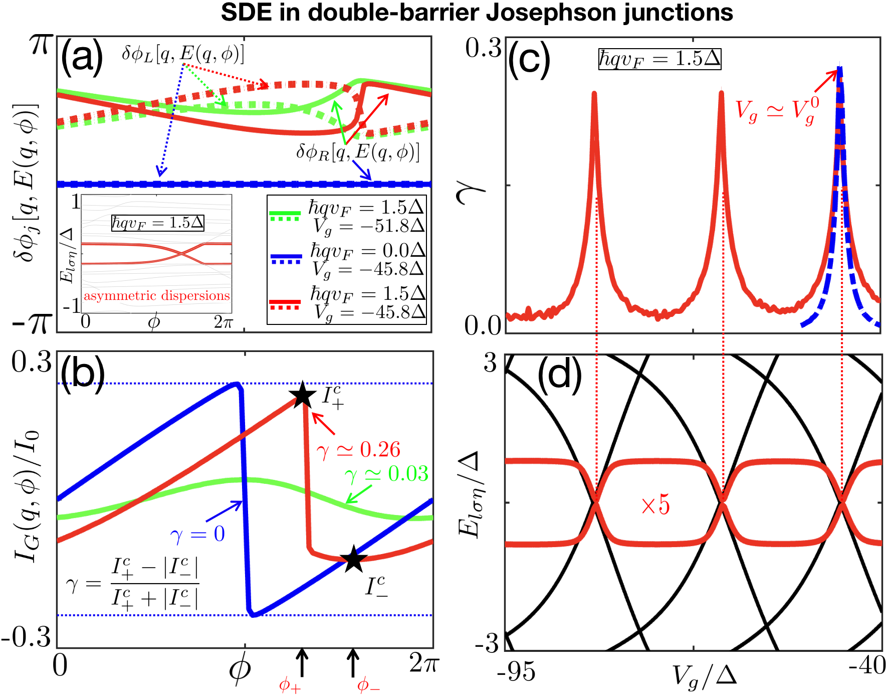
Here we consider a Josephson junction formed by a 1D resonant-tunneling double-barrier InAs semiconducting nanowire placed between two adjacent proximitized InAs/Al superconducting leads [45] with finite momentum Cooper pairing, combining the extraordinary tunability of semiconductors, the remarkable scalability of superconducting circuits, and the compact footprint of quantum dots. Within the Bogoliubov-de Gennes (BdG) formalism, we determine the exact ground-state energy and the accumulated phase shifts Fig. 2(a), due to multiple Andreev reflections, for our phase-biased junction. We also obtain the supercurrent phase relation , from which we extract the depairing supercurrents signaling SDE, Fig. 2(b). The asymmetry about of the phase shifts Fig. 2(a) results in asymmetric dispersions for [inset of Fig. 2(a)] known to originate SDE.
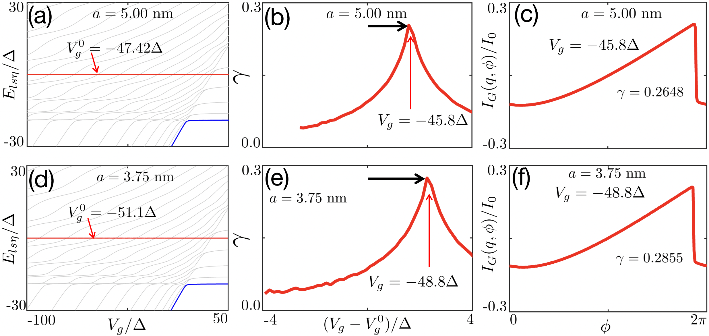
For our resonant-tunneling Josephson junction, we find a sizable SDE with the diode efficiency exhibiting sharp gate-tunable () Fabry-Perot type resonances, peaking at about , Fig. 2(c). These arise from the many zero-energy Andreev bound states [Fig. 2(d), red lines lines] stemming from the ordinary quasi-bound states of the double barrier [Fig. 2(d), black solid lines]. We can further investigate SDE within the simpler single-site quantum dot model for a Josephson junction, Fig. 1(a) (lower part). We find that the SO in the dot-lead tunnel coupling, finite momentum , and Zeeman fields (dot and leads) can substantially affect SDE, thus producing multiple sign reversals in the diode efficiency , Figs. 3 and 4. The Zeeman fields, in particular, can induce fermion-parity (even/odd) transitions of the ground state, which can greatly affect the current phase relation thus significantly changing the SDE, Fig. 3(b). The sharp jumps in vs not only offer signatures for parity changes, but also yield unique switchings within a very narrow phase range, , Fig. 3(b) (green curve). This enables high sensitivity in the SDE tuning, possibly being a resource for superconducting electronics. Furthermore, the dot model yields approximate expressions (via Green functions) for the Andreev bound states, thus providing insight into the crucial role of the phase shifts (see Sec. II.4).
The paper is organized as follows. In Sec. II, we present our model and theory, including the continuum and tight-bind models of double-barrier Josephson junction (Sec. II.1), ground-state supercurrent (Sec. II.2), additional phase shifts in the Andreev reflection of a finite-momentum superconductors (Sec. II.3), as well as single-site quantum dot Josephson junction (Sec. II.4). Section III presents our results and discussions, such as control of SDE via fermion-parity change (Sec. III.1) and tuning SDE via the spin-orbit angle (Sec. III.2). Our paper ends with conclusion and acknowledgement in Sec. IV and Sec. V. The appendices contain detailed information and derivations. Appendix A presents the detailed evolution of the effective Hamiltonian from the continuum (Sec. A.1) to the tight-binding (Sec. A.2) models of the double-barrier Josephson junction, which is then simplified into the single-site quantum dot Josephson junction (Secs. A.3 and A.4). Appendix B and Appendix C provide the detailed derivations of the diagonal Hamiltonian [Eq. (7)] and the ground-state supercurrent [Eq. (10)], respectively. Appendix D presents the additional phase shifts of Andreev reflection in the finite-momentum superconductor, which leads to the microscopic origin of the asymmetric Andreev dispersions discussed in Appendix E. Finally, the investigation of ground state fermion parity changes is presented in Appendix F.
II Model and theory
II.1 From continuum to tight-bind models of double-barrier Josephson junction
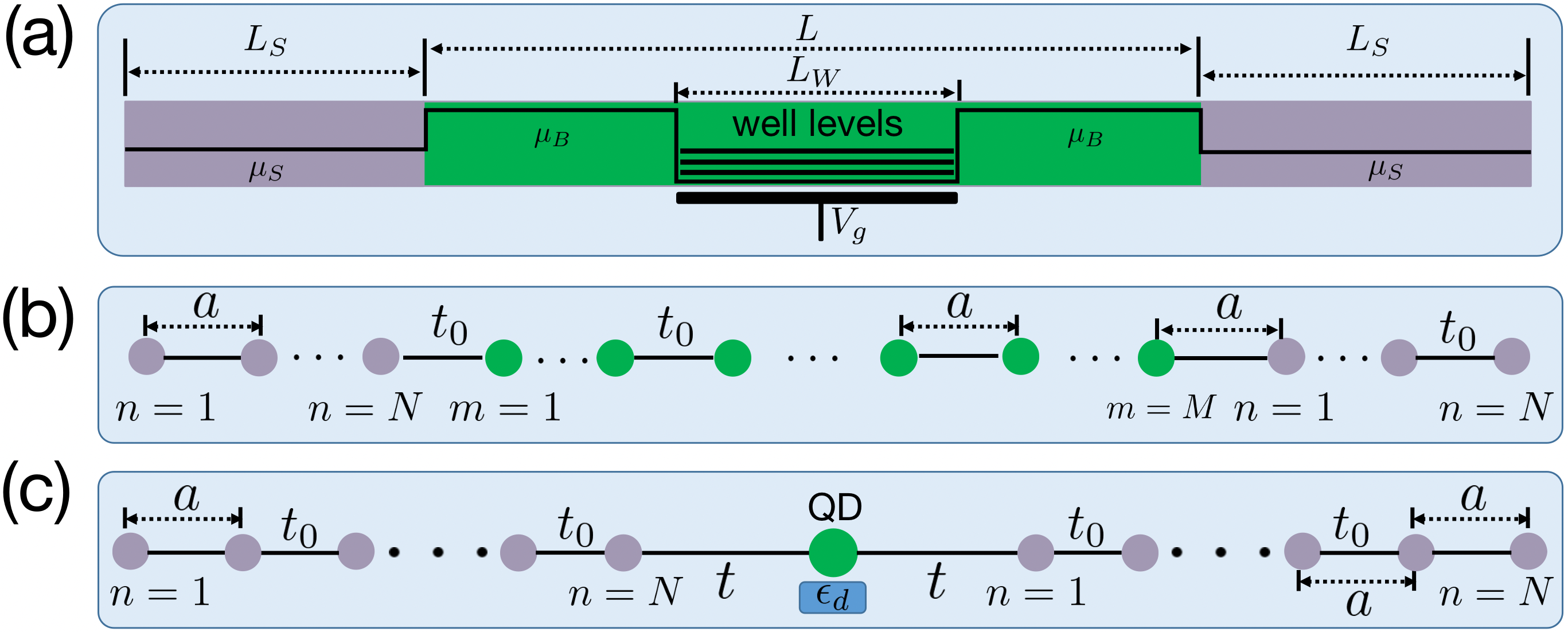
Here, we start with a double-barrier Josephson junction, plotted in Fig. 1(a). The lower panel shows a possible layered structure comprising InAs/Al proximitized superconducting leads with InP barriers and a InAs well [6]. The corresponding BdG Hamiltonian is
| (1) |
where is the electron mass and is the spinor field. The pair potential is zero within semiconductor (green layer) and nonzero within the finite-momentum superconductors (grey layers), i.e.,
| (2) |
where in width of the semiconducting layer. The full chemical potential profile , including the double-barrier structure, is described by
| (3) |
where denotes the well width, the chemical potential of superconductor, the chemical potential of semiconductor, the height of the double barriers, and the electrostatic gate controlling the quantum well depth. For simplicity, we do not consider Zeeman fields and SO coupling in the continuum model; these are included in the simpler single-site quantum dot Josephson junction in Sec. II.4.
By considering the three-point (second derivative) finite difference method with equally spaced discretized points between the end points and , with for , being the (sufficiently small) discretization step, we can approximate the BdG equation of our Hamiltonian (1) by the coupled set of equations
| (4) | ||||
| (5) | ||||
As well known, the three-point second derivative approximation for numerical discretization, e.g., Eqs. (4) and (5), can be formally mapped onto a 1D tight-binding model with nearest-neighbor hopping. More specifically, by making the replacements , , as well as , we can immediately write down the corresponding 1D tight-biding model Hamiltonian
| (6) |
The subscript of electron operator includes the semiconducting (Central) region in addition to the (Left and Right) superconducting leads . The chemical potential define the relevant offsets between the several layers in terms of , , and , as shown by Eq. (3). Here, denotes the respective number of points in the layers, and the total number of sites is given by with and , where is the spacing of the tight-binding mode. The first (last) site () of the semiconductor layer is tunnel coupled to the last (first) site () of the left (right) superconducting lead. The tunnel coupling denotes the nearest-neighbor hopping amplitude in all regions. For the left (right) lead, we assume a Fulde-Ferrell type proximitized order parameter , where and are, respectively, the phase and absolute value of the proximitized gap of the superconducting lead , is the momentum of the Cooper pairs, and is the lattice constant. Below we assume , where is a global flux-tunable phase difference. The finite-momentum Cooper pairs can be realized by, e.g., direct current injection [41, 42, 43], screening currents via the Meissner effect [11, 44], SO interaction + Zeeman field [45], and exchange-mediated Fulde-Ferrel type mechanism [22]. In Appendix A.2.1, we present a detailed explanation and estimation of the mechanism behind the finite-momentum Cooper pairs in our proximitized InAs/Al layer. These pairs can attain significant values of , where represents the Fermi velocity, for experimentally accessible parameters. It is important to note that the momentum of the Cooper pairs should be smaller than the critical dispersing momentum () determined by the closure of the gap in the energy spectra of the continuum quasiparticles. Numerical analysis confirms that , as evidenced by the presence of a clear gap in the energy spectra of the continuum quasiparticles [Fig. 3(a) and the inset of Fig. 2(a)].
II.2 Ground-state supercurrent
The tight-binding Hamiltonian (II.1) is exactly solvable via a (real space) Bogoliubov transformation
| (7) |
where enumerates the dot-lead orbital states and labels the particle-hole degrees of freedom. Here, denotes (pseudo) spin components (if we include spin-orbit coupling in Sec. II.4). The prefactor in Eq. (7) arises from the artificial doubling [46] of the BdG formalism. The quasiparticle eigenenergies and operators are obtained via numerical diagonalization of the BdG Hamiltonian in the -component Nambu spin space ( for all ) and obey particle-hole symmetry and conjugate relation . Hamiltonian (7) is written in the two-quasiparticle representation , with being -independent but dependent on .
Next we obtain the ground state of our system as defined by for all , implying that all positive-energy quasiparticle states are empty in the ground state, i.e., for all . Calculating the ground state of an entangled system is by itself challenging. Further difficulty arises from fermion-parity changes with system parameters. For convenience, we determine the ground state from the effective vacuum state defined by in the orthogonal basis set for all and , with the vacuum energy . This choice of basis suitably guarantees the effective vacuum state has even parity so that the ground state is even for and odd for , [Fig. 3(a)]. Adding all negative-energy quasiparticles [] to the vacuum state , we obtain by construction the ground-state wave function
| (8) |
and, from , the ground-state energy We recast the above as
| (9) |
where we have used . As shown in Appendix C, the ensemble-averaged supercurrent , with being the grand potential function and the temperature [48, 49, 50, 51, 52]. At , [Eq. (9)] and is
| (10) |
where , is the electron charge, , and is the Planck constant. Equation (10) has the great advantage as it enables one to calculate including all negative-only eigenenergies without worrying about parity changes and/or double counting [53, 54, 52].
II.3 Additional phase shifts in the Andreev reflection of a finite-momentum superconductors
Following the same way as Ref. [55], directly diagonalizing the total Hamiltonian (II.4) causes the following reduced determinant equation whose solutions contain exact Andreev levels
| (11) |
The spin degeneracy in Hamiltonian (II.1) halves the dimension of the Hamiltonian matrix and thus is the Hamiltonian matrix of the layer in the Nambu space . The self-energy arises from integrating out the superconducting leads [56]
| (12) |
Here, and are the lowermost and uppermost diagonal blocks of and , respectively,
| (13) |
| (14) |
Each empty square in Eqs. (13) and (14) is a two-by-two matrix, irrelevant to the Andreev levels. Next, we write out , explicitly using their Hermiticity
| (15) |
Hermiticity requires that diagonal Green functions and are real number, which can have different values for the proximitized InAs/Al leads (see Appendix E.2.2). We extract the moduli and phases of the anomalous Green functions by using their polar form
| (16) |
Notably, are additional phase shifts due to the Andreev reflections at the finite-momentum superconducting leads (see detailed explanation in Appendix D). The minus sign in front of in Eq. (15) is added such that when [blue lines in Fig. 2(a)]. Remarkably, the form of the off-diagonal component of the self energy [i.e., Eq. (16)] is quite general. Irrespective of the details of the superconducting leads, their effect on the Andreev reflections are captured by the additional phase shifts that can be numerically calculated.
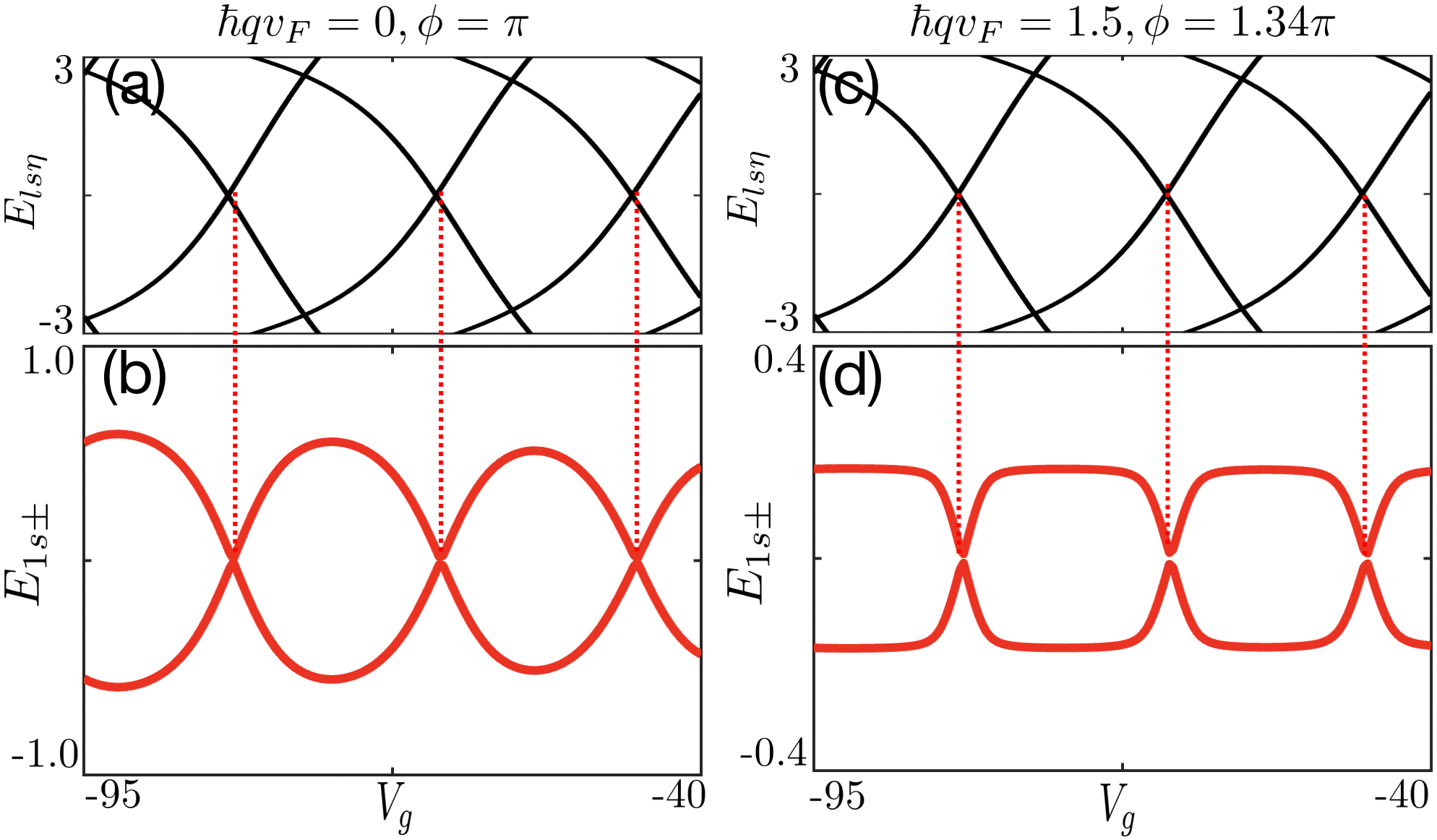
Note that the anomalous Green functions (16) are responsible for the Andreev reflections which couple electrons with holes of opposite spins. As shown in Fig. 1(b), the interference between left- and right-lead Andreev reflections generates phase-tunable Andreev levels and ground-state supercurrent. For finite- leads [red and blue curves in Fig. 2(a)], holes acquire additional phase shifts after the multiply reflections , where the -modulation of the additional phase shifts is introduced by the phase-tunable Andreev levels, e.g., . Notably, these additional phase shifts are asymmetric with respect to , resulting in an asymmetric dispersion [inset of Fig. 2(a)] and a finite SDE [Fig. 2(b)]. Figure 2(b) illustrates vs. [Eq. (10)] for our resonant-tunneling Josephson junction, showing no effect for (blue line) and a sizable SDE for (red and green lines) [1, 14, 21, 9], and reveals that more asymmetric additional phase shifts contribute to larger SDE. Interestingly, the diode efficiency features [Fig. 2(c)] multiple Fabry-Perot resonances due to the many -tunable Andreev bound states [vertical dotted lines in Figs. 2(c) and (d)]. The resonant peaks at in Fig. 2(c) stem from the ordinary zero-energy quasi-bound states of the double-barrier potential [Fig. 2(d), black lines] morphing into Andreev bound states [Fig. 2(d), red lines] due to the superconducting leads. The troughs in Fig. 2(c) have , see green solid line in Fig. 2(b) for . Therefore, we microscopically explain the SDE from the additional phase shifts acquired during the Andreev reflections of finite-momentum superconductors, which exhibits multiple Fabry-Perot resonance.
II.4 Single-site quantum dot Josephson junction
It is important to know that the single-site quantum-dot Josephson-junction model describes well the resonant behavior of ; see, e.g., the peak at [see blue dashed lines in Fig. 2(c)]. In the following analysis, we focus on this simplified single-site quantum dot model, which offers several advantages. Firstly, it allows us to consider the influence of additional parameters such as Zeeman magnetic field and spin-orbit coupling. Moreover, the simplicity of this model enables us to perform analytical calculations, facilitating a better understanding of the underlying physical mechanisms. Below, for simplicity, we only present the 1D tight binding model [11] for a single-site quantum dot coupled to superconducting leads, plotted in bottom panel of Fig. 1(a)
| (17) | ||||
In the presence of the magnetic field, the electron energy in lead is given by , with being the Zeeman energy. The operator annihilates an electron state in the dot having spin component and energy , with and being the dot and Zeeman energies, respectively. The dot energy is assumed to be one of the gate-tunable quasi-bound states , , of the double-barrier potential well. In Figs. 3 and 4, for instance, we take , corresponding to the resonance at in Fig. 2(d). The spin rotation matrix accounts for the spin-orbit induced spin rotation in the tunnelling between the dot and the last (first) site () of the left (right) lead with coupling strength [57, 58, 59, 60, 61]. Noting that is related to the the double-barrier potential, we treat as a fitting parameter to reproduce one of the resonances of the double-barrier Josephson junction.
The natural starting point for studying single-site quantum dot Josephson junction is a superconducting quantum dot described by an effective dot Hamiltonian where the leads are integrated out to generate an order parameter on the dot [62, 63, 64, 65, 66, 67]. Again, we obtain a reduced determinant equation for exact Andreev levels (see detailed derivations in Appendix D.1)
| (18) |
with
| (19) | ||||
where is the spin rotation of the spin-orbit-coupled tunneling in Nambu space. In the absence of the spin degeneracy, and are given by the last and first four-by-four matrix of and , respectively, which are tunnel coupled to the quantum dot
| (20) |
Again, the anomalous Green function is expressed by the polar form, i.e., . In the absence of spin-orbit coupling (), the interference between the left-lead and right-lead Andreev reflections can be captured by
| (21) |
with , where is the additional phase-shift difference from the Andreev reflections in the left and right finite-momentum superconductors. Hereafter, we assume the identical left and right superconducting leads except for the phase of order parameter.
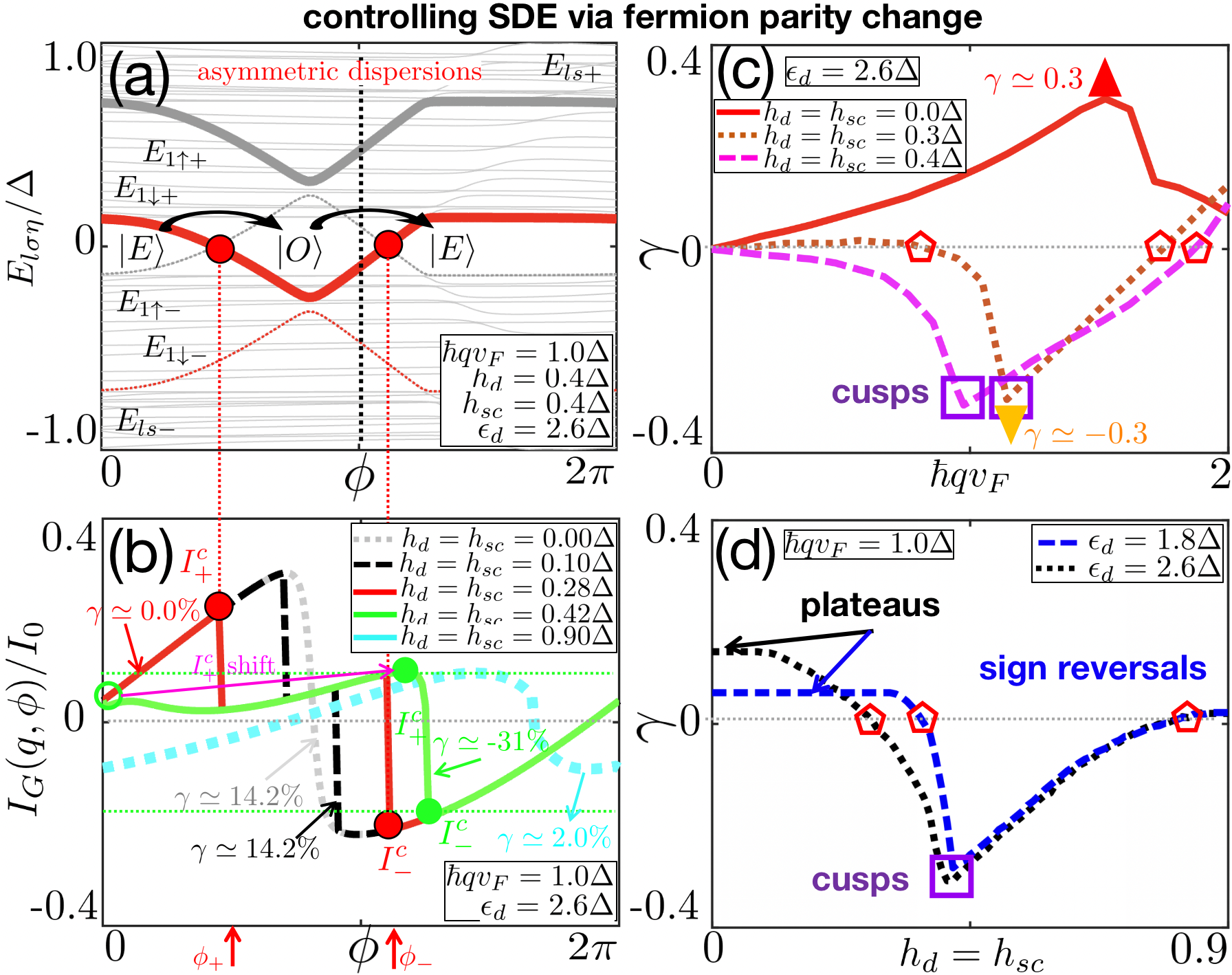
In the absence of Zeeman fields, we have also derived the approximate implicit solution for the Andreev levels of this single-site quantum dot model , where the additional dot energy arises from the renormalization of the lead-dot tunneling coupling (Appendix E.2.2). This clearly shows that the Andreev dispersions are asymmetric about [Fig. 3(a)], due to the asymmetry in [Fig. 2(a)], thus leading to the SDE; here denotes the total dot-lead tunnel rate. Note that above reduces to the known results for . In the presence of Zeeman fields, Fig. 3(a) shows the full BdG spectrum vs. with finite- leads and no spin-orbit coupling in the dot-lead coupling (). The Zeeman fields in the dot and in the leads can cause fermion-parity changes of the ground state due to Zeeman-split negative-energy levels . We find even-odd-even parity transitions at as the subgap levels , cross each at zero energy [see filled red circles in Fig. 3(a)]. In Appendix F.1, we show that , with the functions , , defined following Eq. (146). Parity changes can affect and the SDE as we discuss in Sec. III.1.
III Results and discussions
III.1 Controlling SDE via fermion-parity change
The discontinuities in vs. , see and [red filled circles in Fig. 3(b)], correspond to Andreev levels crossing zero [Fig. 3(a)] and thus signal fermion parity changes. For , these transitions can significantly alter the forward and reverse critical supercurrents , , affecting in turn the SDE [Fig. 3(b)]. For [Fig. 3(b)], we have a finite diode efficiency (gray line). Interestingly, the SDE can be suppressed (red line, ) or enhanced – and even sign reversed (green line, ) – by Zeeman tuning the fermion parity. Note that parity transitions do not affect , when they take place away from the extrema of the current-phase relation ; cf dotted grey line and long-short dashed black line in Fig. 3(b): both have .
Figures 3 (c) and (d) show the diode efficiency as a function of and , respectively. For [red line of Fig. 3 (c)], the maximum efficiency is attained at , which describes a large asymmetry between forward and reverse critical supercurrents . For nonzero fields, shows sign reversals and cusps as increases [Fig. 3(c), see dotted and dashed lines]. Interestingly, for a larger field , becomes fully negative with a cusp () at . Figure 3(d) shows that is initially independent of , because the fermion parity transition does not affect and [see long-short dashed black curve in Fig. 3 (b)]. It then undergoes two sign reversals and exhibits a cusp. The cusp at is due to the shifting closer to as shown in Fig. 3(b) (see arrow connecting the empty and filled green circles). Interestingly, due to this shift, and occur at essentially the same critical phases, i.e., , as shown by the green curve, Fig. 3(b). This should enable phase-tunable SDE devices with high sensitivity over a narrow phase range. It also allows for short switching times between forward and reverse critical currents. The diode efficiency is linear for small [Fig. 3(c)] and its slope can change sign with field. Distinct fields () do not qualitatively change the above results.
III.2 Tuning SDE via the spin-orbit angle
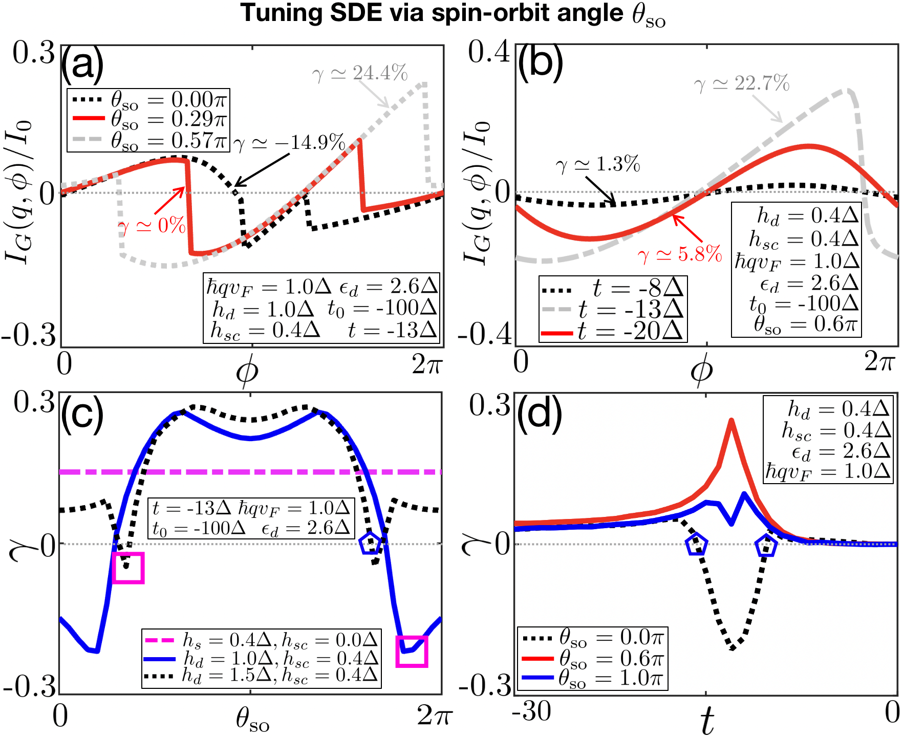
In the presence of spin-orbit interaction in the tunneling between the dot and the leads, spin rotation mixes the spin-dependent Andreev-reflection paths and hence can affect . This couples electrons and holes with opposite and same spins, see gradient arrows in Fig. 1 (b). The spin-rotation unitary matrix accounts for the SO induced rotation in the dot-lead tunneling. Figures 4(a) and (b) show the supercurrent as a function of for different and tunnel coupling amplitude , respectively. For and a vanishing dot Zeeman field and non-zero , Fig. 4 (a), we obtain a sizable SDE with diode efficiency for (black dashed line). As the spin-orbit angle increases, is first suppressed (grey dashed line, ) and then enhanced for (green line, ). Note that varying affects vs. as it significantly alters the fermion parity transition and in turn the forward and reverse critical supercurrents. A similar effect happens when we vary , possibly via an electrostatic gate, as shown in Fig. 4 (b).
The above features are more systematically seen in Figs. 4(c) and (d) showing the diode efficiency as a functions of and , respectively. Interestingly, for , we can rotate the spin basis of the superconducting leads to remove the effect of spin-orbit coupling in the dot-lead tunnel couplings so that the diode efficiency becomes independent of . For finite the spin-orbit significantly modulates the SDE, see the blue curve in Fig. 4(c) with and . For this blue curve we see four sign reversals with increasing , while for a higher dot Zeeman field [red line in Fig. 4 (c)], the diode efficiency is always positive but does show a highly non-linear behavior. Similarly, Fig. 4(d) shows sign reversals and cusps as is varied [cf. Fig. 4(b)].
IV Conclusion
We investigated the SDE in InAs-based resonant-tunneling Josephson junctions with proximitized InAs/Al leads. We find sizable SDE with diode efficiencies showing tunable Fabry-Perot resonances, peaking at . We identify the asymmetry of the phase shifts , due to the multiple Andreev reflections, as the mechanism inducing asymmetric Andreev dispersions and unequal depairing currents . Within a simpler single-site dot model for a Joseph junction, which captures resonant tunneling, we have additionally found that our SDE is highly tunable with exhibiting multiple sign reversals as a function of the SO coupling in the dot-lead tunneling process, Zeeman fields (dot and leads), and finite momentum . Fermion parity transitions can also significantly change SDE. The tunability afforded by our proposed Fabry-Perot superconducting diode should allow the design of new multifunctional devices for future superconducting electronics.
V Acknowledgements
We sincerely thank J. Carlos Egues and Yugui Yao for helpful and sightful discussions. This work was supported by the National Key R&D Program of China (Grant No. 2020YFA0308800).
Appendix A Effective Hamiltonians
In this section discuss the Hamiltonians used to obtain the results in the main text. We first present the continuum model consisting of a semiconducting double-barrier potential sandwiched between two proximitized superconducting leads within the BdG formalism. We then discuss the equivalent lattice tight-binding model describing such a structure in the limit of vanishing lattice parameter taken to be the discretization step (three-point finite differences) of the continuum model. Finally we describe the tight binding model for a Josephson junction with just one resonant level, i.e., a single-site dot coupled to two superconductors. This simpler model captures the essential feature of the continuum description of the double-barrier Josephson junction, i.e., resonant tunneling. It allows the inclusion of additional features in the model (e.g., Zeeman fields in the dot and leads and SO interaction) to more easily investigate the SDE in terms of the corresponding parameters.
A.1 Continuum BdG model for the resonant-tunneling Josephson junction
Figure 5(a) shows the hybrid proximitized-superconductor/semiconductor resonant-tunneling Josephson junction investigated here. The corresponding BdG Hamiltonian is
| (22) |
wher is the electron mass and the spinor field
| (23) |
The pair potential is zero within semiconductor (green layer) and nonzero within the finite-momentum superconductors (grey layers), i.e.,
| (24) |
where in width of the semiconducting layer, [Fig. 5 (a)]. The full chemical potential profile , including the double-barrier structure, is described by
| (25) |
where denotes the well width, the chemical potential of superconductor, the chemical potential of semiconductor, the height of the double barriers, and the electrostatic gate controlling the quantum well depth. The origin is defined at the center of the double barrier potential, Fig. 5(a). For simplicity, we do not consider Zeeman fields and SO coupling in the continuum model; these are included in the simpler single-site model described in the main text. Here, we consider the system size of m and nm, and hence the total number of sites is given by , where and , where is the spacing of the tight-binding mode (Fig. 5).
A.2 Discretized continuum model as a 1D nearest-neighbor tight-binding model
By considering the three-point (second derivative) finite difference method with equally spaced discretized points between the end points and , with for , being the (sufficiently small) discretization step, we can approximate the BdG equation of our Hamiltonian (22) by the coupled set of equations
| (26) |
The pair potential couples the spin-dependent components of the field spinors and . A more familiar form of Eq. (A.2) is
| (27) |
where we have used the discretized versions of the relevant quantities: , and . As well known, the three-point second derivative approximation for numerical discretization, e.g., Eq. (27), can be formally mapped onto a 1D tight-binding model with nearest-neighbor hopping, similar to the one introduced in the main text for the single-site dot. More specifically, by making the replacements
| (28) | ||||
| (29) | ||||
| (30) |
we can immediately write down the 1D tight-biding model corresponding to Fig. 5(b)
| (31) |
Note that the subscript of fermionic electron operator includes the semiconducting (Central) region in addition to the (Left and Right) superconducting leads . The field operator annihilates a spin- electron at position in region . Here denotes the respective number of points in the layers, i.e., and . For definiteness, we index the superconducting leads with (similar) indices and the central semiconducting region with index . The first (last) site () of the semiconductor layer is tunnel coupled to the last (first) site () of the left (right) superconducting lead. The tunnel coupling denotes the nearest-neighbor hopping amplitude in all regions. For the left (right) superconducting lead, we consider the Fulde-Ferrell type order parameter
| (32) |
where is the Cooper-pair momentum of the superconducting lead with global superconducting phase , and is the lattice constant.
A.2.1 Tight-binding dispersions in the normal leads and some estimates
For clarity and definiteness of the parameters used in the main text (e.g., Fermi wave vector and energy), next we show the energy bands for normal leads. In this case, the tight binding bands (left and right leads), assuming periodic boundary conditions with wave vector , are give by
| (33) |
where we have straightforwardly Fourier transformed the first two terms of Eq. (31). The above expression shows that the bottom of the band (we use in the main text) is , while the Brillouin zone edge is . In this case, a half-filled band corresponds to a Fermi wave vector . In our simulations, we are always away from half filling. Because we are interested in InAs-based semiconducting systems, we choose a closer to the bottom of the band, e.g., in Fig. 2. In this case, we can approximate the above dispersion by expanding it to second order in k
| (34) |
We can then define an effective mass
| (35) |
Assuming for InAs-based systems [45], we find meV (this is the value we use in Fig. 2). By using a typical electron density cm-2 in InAs-based wells [45], we can estimate the magnitude of Fermi wave vector for a 2D electron gas, . If we use, instead, for a 1D electron gas and consider cm-1 [68], we obtain nm nm. In our simulations, we take , with lattice parameter nm so that nm-1 (20% of the Brillouin zone) for which the quadratic dispersion is valid. This number is consistent with the above estimates for based on the electron density. We note that the nm used here corresponds to a small enough step so that the numerical solution is converged; in the next subsection we discuss convergence in more detail.
Coherence length . The proximitized InAs/Al is given by superconductor is
| (36) |
Since (eV ), with eV and , we can write
| (37) |
Note that
| (38) |
To estimate the chemical potential of the superconductor, we define the Fermi energy as the zero of energy, i.e.,
| (39) |
Using nm-1, which is consistent with the usual electrons densities in InAs-basel well and wires [68], we find meV from Eq. (39), which is similar to meV the numbers we used to generate Fig. 2 with energy dispersion (33).
Estimate of the parameter . As mentioned in the main text, parametrizes the finite momentum of the Cooper pairs that, in principle, can generate (an anomalous) supercurrent at . Cooper pairs with a finite momentum can arise from, e.g., (i) the interplay of (Rashba) spin-orbit interaction and Zeeman field in InAs-based proximitized 2D electron gases [39, 45], (ii) screening currents (Meissner effect) due to a weak external magnetic field [11, 44], (iii) orbital effects leading to the acquision of an inhomogeneous phase [69], (v) exchange interaction [22], (iv) injected current only [41, 42, 43]. In our proximitized InAs/Al nanowire system, Cooper pairs originating from the Al layer can leak into the InAs region, inducing superconductivity in InAs. When an external magnetic field is applied perpendicular to the InAs/Al nanowire, the Meissner effect leads to the formation of unidirectional edge screening currents, similar to the edge current of quantum Hall effect. These screening currents result in the presence of finite-momentum Cooper pairs that also leak into the InAs nanowire. Consequently, we observe the existence of finite-momentum Cooper pairs in the proximitized InAs. The momentum of these Cooper pairs arising from this mechanism can be estimated using the expression [11]. For a sizable London penetration depth nm [70], a magnetic field of approximately mT is required to generate sizable momentum [44]. Importantly, this momentum is much smaller than the Fermi momentum , i.e., . Here, we have utilized experimentally available parameters, including the order parameter meV, Fermi momentum nm-1, Fermi velocity m/s, and effective mass (consistent with the parameters employed in all figures).
A.2.2 Numerical convergence of the continuum model.
Recall that in the continuum model is the discretization step to be chosen sufficiently small so that the eigenvalue solution is convergent and, in turn, so are all other calculated (physical) quantities. Figures 6 (a), (b), and (c) illustrate the evolution of this convergence (different ’s) for the ground-state supercurrent [Eq. (6) of main text] vs. the phase difference . We obtain a convergent result for sufficiently small spacing nm [Fig. 6 (c)].
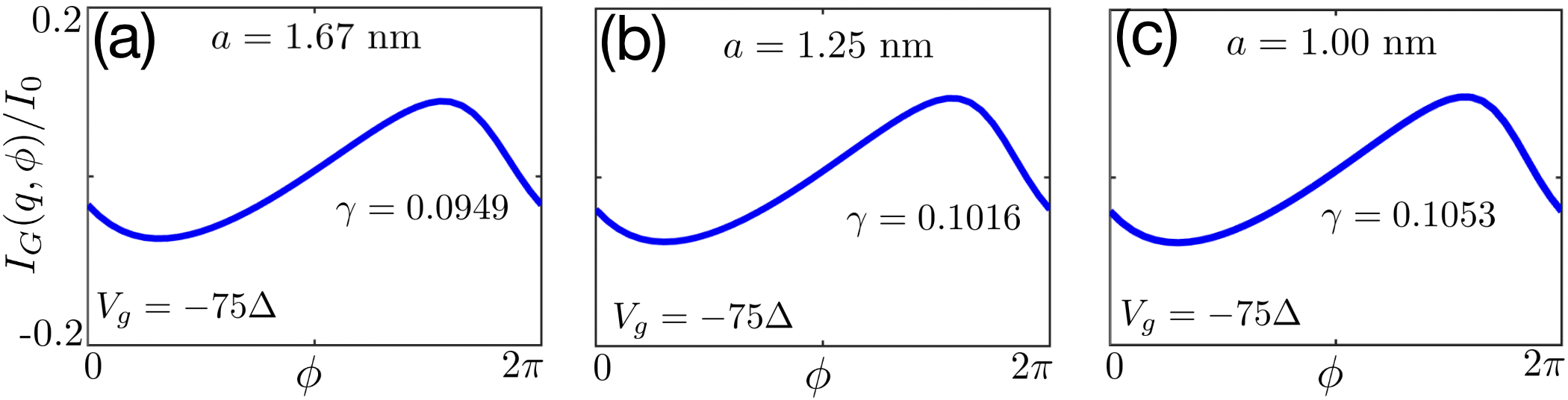
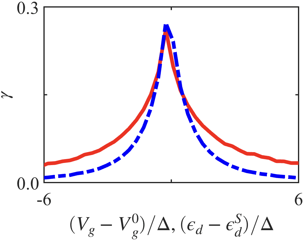
However, the convergent result numerically calculated from the tight-binding model (31) requires huge system sites (see Fig. 6) and hence costs long time for numerical calculations. Figure 7 plots the bare quasi-bound states, diode efficiency, and current-phase relation for smaller spacing. We note that the maximum diode efficiency is shifted to the right-hand side due to the renormalization of effective well bound-state energy from the lead-dot tunneling coupling, as shown by the black arrows in Figs. 7 (b) and (e). This renormalization depends on [Eq. (139)] and hence varies with via [Eq. (28)] when is not small enough. This shift is well-explained in Sec. E. The current phase relations at the maximum diode efficiency are plotted in panels (c) and (f). Though they are not perfect convergent results, all of them qualitatively show same behaviours, the shifted resonant tunneling and current-phase relation. Therefore, in the main text, we use a larger spacing nm, which can capture the main physics in our model.
A.3 Gate-tunable Andreev levels
Here we explore how the gate voltage controlling the well depth tunes the Andreev levels of our hybrid semiconductor-superconductor Josephson junction. Figure 8 shows the dependence of (a) the ordinary quasi-bound states of the double-barrier potential well in the absence of superconductivity and (b) the corresponding Andreev bound states of our Josephson junction for and . Figure 8(c) (repeated on the right panel for convenience) is identical to Fig. 8(a), while Fig. 8(d) is similar to Fig. 8(b) but for finite momentum and . For the Andreev levels touch each other as the superconducting gap closes at and oscillate as a function of . Interestingly, gap closing is now periodic in and happens whenever one of the -tunable quasi-bound states of the well crosses zero [vertical red dashed lines in (a),(b)]. For this gap closing takes place at because the Andreev spectrum is asymmetric for . Similarly to the case, Andreev levels are still highly tunable for and successively cross the zero-energy baseline as the well depth is varied [vertical dashed lines (c) and (d)]. Unlike the case, the Andreev levels ) feature flat regions as a function of due the avoided crossing between tunable quasi-bound state of the well and the gap edge of the finite-momentum superconducting lead; cf. solid red lines in (d) and (b).
A.4 From a multi-level double-barrier quantum well to a single-site quantum dot
As mentioned in the main text and at the beginning of this section, we would also consider a simpler 1D tight binding model describing a single-site quantum dot Josephson junction as a means to further investigate SDE considering additional parameters. This is illustrated in Fig. 5(c). The single-site dot model retains just one of the resonances of the continuum model, which is selected by choosing to coincide with one of the double-barrier well quasi-bound levels. Below, for completeness, we reproduce the 1D tight biding model for the single-site dot coupled to superconducting leads shown in Eq. (1) of the main text,
| (40) |
Physically, the tunnel coupling between the quantum dot and superconducting leads is related to the the double-barrier potential [Eq. (25)] of the continuum model. Here we treat as a fitting parameter to reproduce one of the resonances of the continuum model. Figure 9 shows the resonance peak in the diode efficiency obtained via the continuum model (red solid line) and the single-site quantum dot model (blue dotted line). The parameters used in both simulations are listed in tables 1 and 2. The spin rotation matrix is responsible for accounting for the spin rotation induced by spin-orbit coupling () during the tunneling process between the quantum dot and the last (first) site () of the left (right) lead. Spin-orbit coupling exists in both the semiconducting quantum dot and the proximitized InAs/Al leads, creating an effective magnetic field that leads to a momentum-dependent spin rotation of itinerant electrons. In our work, the purpose of the single-site quantum dot Josephson junction is to obtain approximate expressions for the Andreev levels using Green functions. This approach allows us to gain insight into the important role played by the phase shifts (refer to Sec. II.3). To achieve this objective, we incorporate the effect of spin-orbit coupling on the Andreev levels in a simple manner, treating it as a spin rotation during the tunneling process between the quantum dot and the superconducting leads. It is worth noting that the Andreev levels are derived from the reduced determinant equation [Eq. (18) and Eq. (94)], where the degrees of freedom associated with the superconducting leads are integrated out to generate a self-energy term that captures the overall influence of the superconducting leads on the Andreev levels. Interestingly, the form of the self-energy [Eq. (19)] is quite general and does not depend on the specific details of the superconducting leads. As a result, this spin rotation approach effectively encapsulates the effects of spin-orbit coupling from both the semiconducting quantum dot and the proximitized InAs/Al leads on the Andreev levels.
| 0.5 meV | -50 meV | 2000 | -19 meV | 5 nm | 0.03 | 0.45 m | 0.15 m | 9 meV | -23 meV |
| 0.5 meV | -50 meV | 2000 | -19 meV | 5 nm | 0.03 | -6.5 meV | 1.3 meV |
Appendix B Derivation of the Hamiltonian [Eq. (7)] in the main text
In this section, we write out the Bogoliubov-de-Gennes (BdG) Hamiltonian, corresponding to in Eq. (II.4), in Nambu-spin space and detail the steps to formally derive Eq. (2) in the main text.
B.1 Generalized Nambu field operator and the BdG Hamiltonian
Let us rewrite the total Hamiltonian [Eq. (1) in main text] in the Nambu space of the hybrid quantum-dot/superconducting-lead system described by the field operator
| (41) |
where and , denote the field operators for dot and superconducting leads, respectively. More explicitly, we have
| (42) |
where concatenates vertically. Using the generalized Nambu field operator above, we can straightforwardly recast [Eq. (1), main text] in the form
| (43) |
where the BdG Hamiltonian matrix is given by
| (47) |
and
| (48) |
is a -independent constant (recall that is the site energy, Eq. (1) in the main text). The factor of 1/2 in Eq. (43) arises from the artificial doubling in the BdG formalism [46]. The quantum dot is described by the non-interacting Hamiltonian
| (49) | ||||
where and are Pauli matrices acting within the Nambu and spin spaces, respectively. The Hamiltonian describes the superconducting leads ,
| (50) |
with
| (51) |
| (52) |
denotes the dot-lead tunnel coupling amplitude, and
| (53) |
where
| (54) |
and the finite- superconducting pairing gap
| (55) |
For simplicity, in what follows, apart from distinct phases , , we assume otherwise identical left and right superconducting leads. The tunnel-coupling matrix between the quantum dot and the left and right leads are, respectively,
| (56) |
| (57) |
where the unitary matrix accounts for the spin-orbit (SO) effect in the tunneling processes (left and right) and is given by
| (58) |
with describing the spin rotation due to the spin-orbit coupling in the tunneling between the quantum dot and superconducting leads.
By numerically diagonalizing the BdG matrix (47) we can construct the -dependent Bogoliubov (quasiparticle) operators as unit vectors in the Nambu space (42), i.e.,
| (59) |
where is the th component of in Eq. (42) and is the -th eigenvector that diagonalizes the BdG Hamiltonian; the Bogoliubov operators obey the conjugation relation
| (60) |
We can now recast the total Hamiltonian (43) in the form of Eq. (2) in the main text,
| (61) |
Note that in the above the quasi-particle eigenenergies depend only on the phase difference and satisfy,
| (62) |
due to particle-hole symmetry. To see that the eigenenergies depend on the phase difference , let us do the transformation , and in Eq 1 (main text). The pair potential then transforms as while the tunnel coupling between the dot and left (right) superconducting lead transforms as (). Thus, the eigenenergies depend on only the phase difference [note that a term does not appear in the transformed Hamiltonian.]
In the main text, we use the orthogonal basis set as this choice makes it straightforward to determine the ground-state wave function and energy . Using Eqs. (60) and (62), we can replace all with in the Hamiltonian (61) to obtain its form in this basis,
| (63) |
where
| (64) |
is the -dependent energy of the vacuum state . The form in Eq. (63) is also convenient for the calculation of the ensemble-averaged supercurrent (Sec. (C.2)).
Appendix C Derivation of Eq. (4) (main text) for the supercurrent
For completeness, in this section, we derive the supercurrent in Eq. (6) of the main text following Ref. [71, 72].
C.1 Current definition
Quite generally, in terms of the time evolution of the electron number operator in the left lead , we can define current as
| (65) |
where is given in Eq. (1) in the main text and (see below) is its tunnel coupling part. The angle bracket in Eq. (65) denotes either (i) the expectation value in the ground state [e.g., Eq. (3) in the main text for our problem] at zero temperature () or (ii) the grand-canonical ensemble average for non-zero , is the charge of the electron and is the reduced Plank constant. Here we use the subindex “’ in as our focus in the main text is the ground-state () supercurrent. Equivalently, we can define current from the electron number operator in the right lead ,
| (66) |
Using
| (67) | |||
which follows from the self-consistency condition of the order parameter, Eqs. (65) and (66) become
| (68) |
To calculate the commutators in Eq. (68), we first do the transformation and in Eq. (1), main text, which leads to
| (69) | |||
and
| (70) | ||||
| (71) | ||||
| (72) |
| (73) | |||
we find the identity
| (74) |
Using [Eq. (68)], we can write the above as
| (75) |
Hence the current (65) becomes
| (76) |
where we have explicitly written out the and dependencies of [there is also, in principle, a temperature dependence (not indicated) in the case we are considering a thermal average (Sec. C.2)]. Since we are dealing with a superconducting system with no voltage applied, we will hereafter refer to in (76) as supercurrent.
C.2 Thermal average of the supercurrent in the grand-canonical ensemble
Even though we are interested in the zero-temperature limit () in the main text, here we calculate the supercurrent in Eq. (76) by performing an ensemble average in the grand-canonical ensemble. As we see below, besides being instructive, this provides, as a bonus, an alternative way to obtain the ground-state energy of our system.
The grand potential function is defined as
| (77) |
with being the grand partition function. More explicitly, using in Eq. (63), we have
| (78) |
The ensemble-averaged supercurrent [Eq (76)] can be expressed as
| (79) |
with
| (80) |
Note that the pre-factor appears naturally in the supercurrent (C.2), obtained quite generally from (65) or (66).
C.2.1 limit of ): ground-state energy
In the () we have
| (81) |
Interestingly, in this limit the grand potential [Eq (80)] reduces to the ground-state energy [Eq. (5) in the main text], i.e.,
| (82) |
where is defined in Eq. (64). Note that the above result, more than just yielding the correct limit, provides an alternative way to derive the ground-state energy . In the main text, we derived from the exact ground-state wave function [Eq. (3)] via . As mentioned in the main text, since , we can replace all positive energies in (82) [and in (64)] with negative eigenenergies to obtain
| (83) |
where is the constant defined in Eq. (48), being independent of and . Note that the form of in (83) is particularly convenient to calculate the ground-state supercurrent (see below) as its -dependence is solely included in the second term, which involves only negative quasi-particle eigenenergies.
C.2.2 limit: ground-state supercurrent
Appendix D Additional phase shifts in finite- superconductors
In this section, we define the additional phase shifts , central to our discussion and plotted in Figs. 1(b) and 1(c) of the main text, in terms of the matrix elements of the anomalous Green functions of the finite-momentum superconducting leads. To this end, below we focus on an effective description of the quantum dot in which the effect of the leads are accounted for via a self energy. We derive a general expression for the self energy that incorporates the phase shifts via the superconducting lead (anomalous) Green functions. As we will see later on, these phase shifts (via the self energy) provide a simple mechanism to understand (i) the finite--induced asymmetry of the Andreev dispersions [Sec. (E)], crucial to the SDE, and (ii) the fermion parity changes in the ground state [Sec. (F)]
D.1 Defining an effective dot Hamiltonian and self energy
A simpler starting point for studying Andreev bound states in our hybrid quantum-dot/superconducting-lead system is to consider an effective quantum dot Hamiltonian in which the leads have been integrated out thus giving rise to a self energy, which, as we will see below, emulates a pair potential in the quantum dot [62, 63, 64, 65, 66, 67]. To this end, we note that the diagonalization of the BdG matrix (47) results in the determinantal equation,
| (89) |
To find the Andreev (subgap) levels we can use the identity for determinants of block matrices comprised of four matrices , and [56],
| (90) |
where is assumed to be invertible. By comparing Eqs. (89) and (90) we can make make the identifications: , , , and
| (93) |
Now we have to guarantee that the blocks (i.e., block ) are invertible. As it turns out, this is the case for Andreev eigenenergies (i.e., for in-gap ’s). In this case, Eq. (89) [via Eq. (90)] reduces to
| (94) |
where we have introduced the self energy
| (95) |
Note that the determinantal Eq. (94) can be viewed as stemming from the effective quantum-dot 4x4 Hamiltonian,
| (96) |
in which the superconducting leads have been eliminated thus giving rise to the self energy (D.1). Interestingly, this self-energy emulates a pair potential in the quantum dot [via , see Eqs. (50)and (53)].
Here we derive an expression for the dot self energy (D.1) making more explicit the contributions from the left and right leads. By using Eqs. (56) and (57), Eq. (D.1) becomes
| (97) |
The quantum dot is coupled to the last site of the left superconducting lead and the first site of the right superconducting lead, as shown by the first and second lines of Eq. (D.1), respectively, and hence only the last block of and the first block of participate in the calculation of the self-energy (D.1). More explicitly, below we specify the lowermost and uppermost 4x4 diagonal blocks of , denoted by and ,
| (98) | ||||
| (99) | ||||
Each empty square in Eqs. (98) and (99) is the matrix
| (100) |
In the upper and lower diagonal 2x2 blocks of above, the triangles denote couplings between only same spins, while in its off-diagonal 2x2 blocks Cooper pairing couples only opposite spins, see Eq. (53). Substituting Eqs. (98) and (99) into (D.1), we obtain the general expression for the self energy
| (101) |
The first and second terms on the right-hand side of (D.1) correspond to the contributions from the left and right leads, respectively.
D.2 Additional phase shifts
Here we write out the blocks , [Eqs. (98) and (99)], explicitly making use of their hermitian properties. By introducing diagonal and off-diagonal matrix elements we can write
| (102) |
where we have omitted the , , and dependencies of the matrix elements for simplicity. The off-diagonal functions correspond to anomalous matrix elements of the superconducting leads. Note that all Green functions in Eq. (102) [also in Eqs. (98) and (99)] have a magnetic field dependence [see, Eqs. (50), (53) and (54)]; whenever discussing non-zero effects, we should make the substitution in Eq. (102) to make the dependence explicit. As usual, hermiticity requires that the diagonal Green functions () be real numbers.
The anomalous Green functions , on the other hand, can in principle be complex, where . To extract the moduli and phases of , we use their polar form
| (103) |
where denote their phases. By comparing the numerically determined with Eq. (103), we can determine the moduli and phases . The minus sign in front of in Eq. (102) is added so that when .
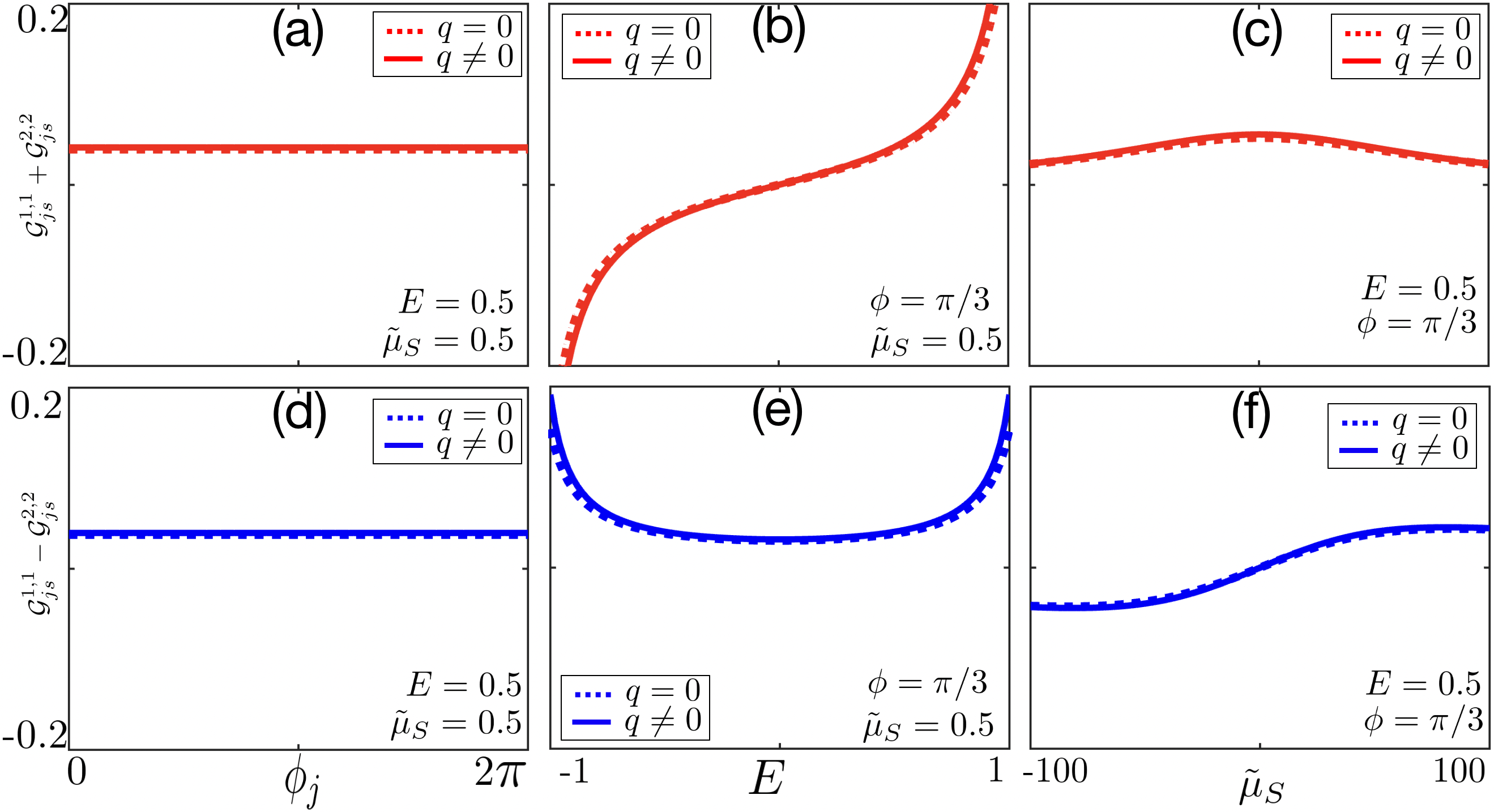
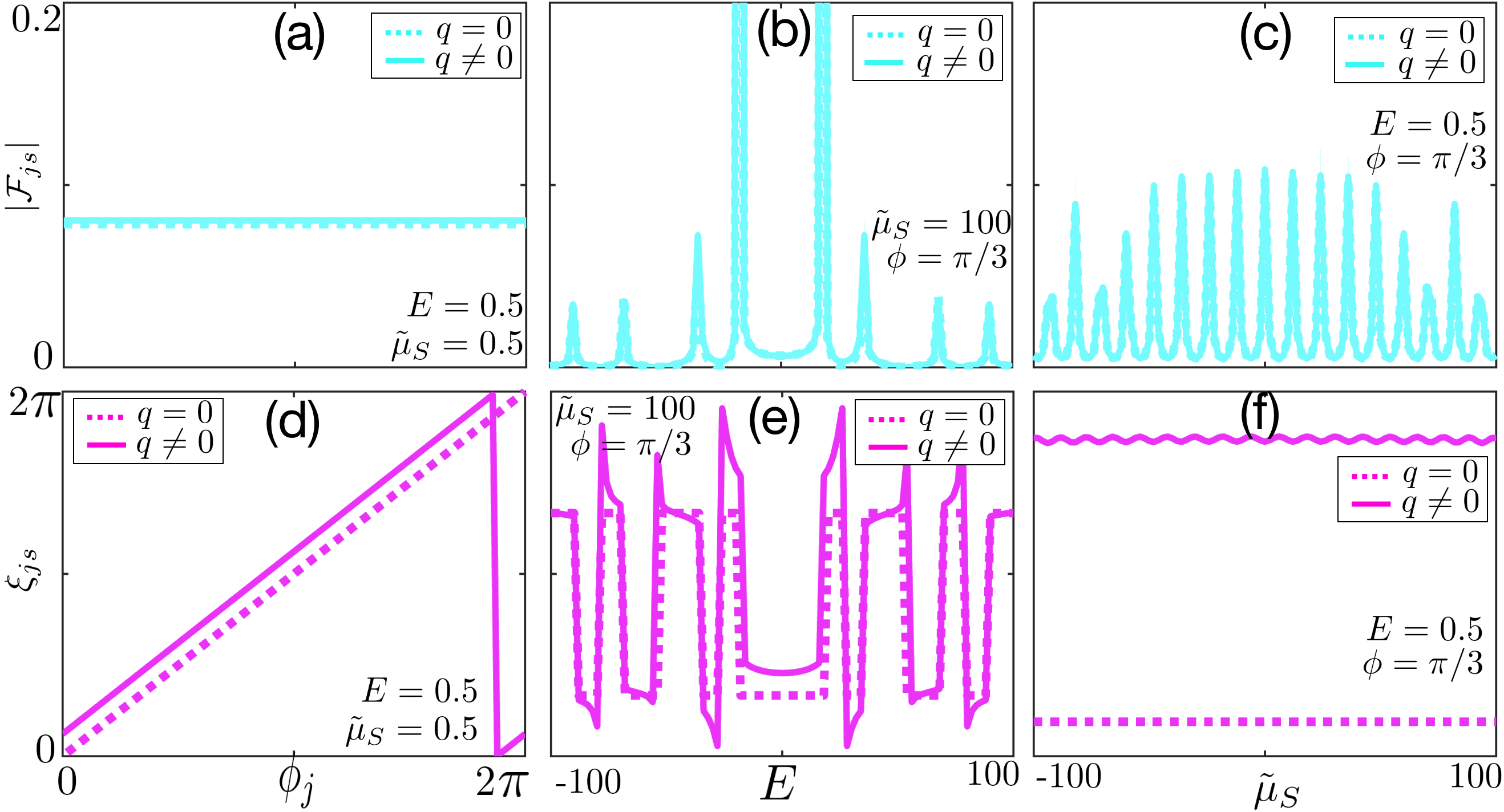
Figure 10 (a) shows as a function of phase for different values of . Figures 10 (b) and (c) are similar to Fig. 10 (a) but as a function of the energy and , respectively. Panels (d), (e), and (f) correspond to (a), (b), and (c) but for . Note that the Green and [i.e., ] are independent of for both and , as shown in Fig. 10(a) and Fig. 10(d), respectively. From Figs. refAFIGG (b) and (e) we see that is an odd function of but is an even function of . While is an even function of [Figs. 10 (c)], is an odd function of [Figs. 10 (f)]. Figs. 11 (a), (b), and (c) correspond to Figs. 10 (a), (b), and (c) but for . Figures 11 (d), (e), and (f) correspond to (a), (b) and (c) but for . From Fig. 11(a), we see that the moduli of the anomalous Green functions are independent of . It becomes even functions of and , as shown in Figs. 11(b) and (c). Their phases are linear in [Figs. 11(d)] for and . These phases are independent of for , while strongly energy dependent for , as shown in Fig. 11(e). Thus, we suggest the ansätz
| (104) |
where are additional phase shifts due to the Andreev reflections in the finite-momentum superconducting leads. These phase shifts, as it turns out, do not explicitly depend on . As we will see in the next section, the additional phase shifts
| (105) |
play an important role in giving rise to asymmetric Andreev dispersions, which, in turn, underlie the SDE in our Andreev QD setup.
To obtain a more compact and convenient form for further calculations involving , let us define the operation
| (106) |
where denotes a generic matrix. Using this notation and Eq. (104), we can now recast the blocks in Eq. (102) as
| (107) | ||||
where we have defined the functions
| (108) |
| (109) |
| (110) |
In the above we have explicitly put in the dependence on the magnetic field in the arguments of the functions , and ; note that these are real functions, being independent of , see Fig. 10 and Fig. 11.
Appendix E Origin of the asymmetric Andreev dispersions for finite
To gain some insight into how the finite-momentum of the Cooper pairs affects the Andreev reflections, and, in particular, how it leads to asymmetric dispersions, below we look in some detail at the simpler case with no Zeeman fields () and no spin-orbit coupling ().
E.1 Self energy for
First of all let us write out the self energy for this case in terms of the matrix elements of the superconducting lead Green functions. Substituting Eq. (107) into the self-energy (D.1), we obtain
| (111) |
where we have defined,
| (112) | ||||
The above describes the interference between the Andreev reflections in the left-lead and right-lead paths [Fig. 1(b), main text] and can be rewritten as
| (113) | ||||
with , where is the flux-tunable phase difference between the left and right superconducting leads and is the additional phase-shift difference between the left and right phase shifts arising from the Andreev reflections in the left and right finite-momentum superconductors. Remarkably, the form of the off-diagonal component of the self energy [i.e., Eq. (113)] is quite general. Irrespective of the details of the superconducting leads, their effect on the Andreev reflections are captured by the additional phase-shift difference that can be numerically calculated.
E.2 Andreev dispersions for
By substituting the self energy (111) into Eq. (94), we can determine the Andreev in-gap states from the secular equation
| (114) |
where dropped out. Equation (E.2) can be formally solved as an implicit solution for the Andreev eigenenergies ,
| (115) |
with . From the compact implicit equation above we can obtain the Andreev levels, e.g, iteratively. Note that . Here, the phase shifts obey particle-hole symmetry, i.e., , as shown by Fig. 11 (e).
Note that , and are complicated functions and can only be calculated numerically. To have some analytical result, let us perform the transformation of the fermionic lead operators
| (116) |
with
| (117) |
The above corresponds to a change of basis in the leads, i.e., from the original site (position) representation to the k-space representation. Substituting Eq. (116) into the superconducting lead Hamiltonian (c.f., Eq. (1) in the main text)
| (118) | ||||
we obtain
| (119) |
where we have use the identity (117). In the limit of , we can omit the third line of Eq. (E.2) for simplicity and therefore the lead Hamiltonian (E.2) becomes diagonal in space. We denote the -space version of the Nambu space of the superconducting leads by adding a superscript to ,
| (120) |
The transformation (116) does not change the many-body Hamiltonian of our system [(43)] but it does change the representation of the Bogoliubov Hamiltonian , (47). As a matter of fact, only does note change; all the other blocks of , i.e., , , , and do change. Below we add a superscript in all these matrices so as to emphasize the k-space representation used in the leads.
| (121) |
with
| (122) |
where
| (123) |
is the energy spectrum of the lead . The tunnel-coupling matrix between the quantum dot and the left and right leads in the Nambu basis (120) are, respectively,
| (124) |
| (125) |
where the tunneling matrix is given by Eq. (51). Note that the real-space coupling between the dot and the last (first) site of the left (right) lead, translates into a -independent tunnel coupling matrix in the -space representation of the leads. Following the same procedure as in Eqs. (89-94), we obtain the self-energy of the Andreev quantum dot
| (126) | ||||
We emphasize that the above self energy is exacly the same as the one calculated in the real-space site representation, Eq. (D.1). This is so because we performed the change of basis (k-space) only on the leads. Substituting Eqs. (121) and (122) into the self-energy (126), we obtain
| (127) | ||||
Note that is diagonal in space [see Eq. (121)]. The huge matrix calculation of the above self-energy can be written as a summation over
| (128) | ||||
| (131) |
where is the Pauli matrix in Nambu space. Let us define the Green functions as follows
| (134) | ||||
| (135) |
where . The self-energy (128) then becomes
| (136) |
E.2.1 Zero Cooper pair momentum: symmetric dispersions
Here, for simplicity, we first consider the case with zero Cooper pair momentum .
The summation over momenta in each element of the self-energy (136) can be replaced by integration as follows
| (137) |
where is the density of states of superconductor per spin. Then, Eq. (136) reduces to
| (138) |
with
| (139) |
We have and , where and is the density of states of superconducting leads at the Fermi energy for each spin species and is assumed to be -independent for simplicity. Then, the Andreev levels (115) becomes
| (140) |
Obviously, Andreev levels at [Eq. (140)] is a symmetric dispersion, i.e., . As a result, if we find a critical forward supercurrent at , we can always obtain a critical reverse suppercurrent at with the same magnitude, i.e., . Note that the superconducting lead-quantum dot tunneling coupling renormalizes effective dot energy , superconducting proximity effect with effective pair potential , as well as Andreev levels [it appears in the denominator of the Andreev levels (115)]. In weak tunneling and low energy limit (), the renormalization effects from become independent of , and the above Andreev level reduces to . Thus, we obtain better agreement for smaller as shown by the red lines in Figs. 12 (a).
E.2.2 Finite Cooper-pair momentum : asymmetric dispersions
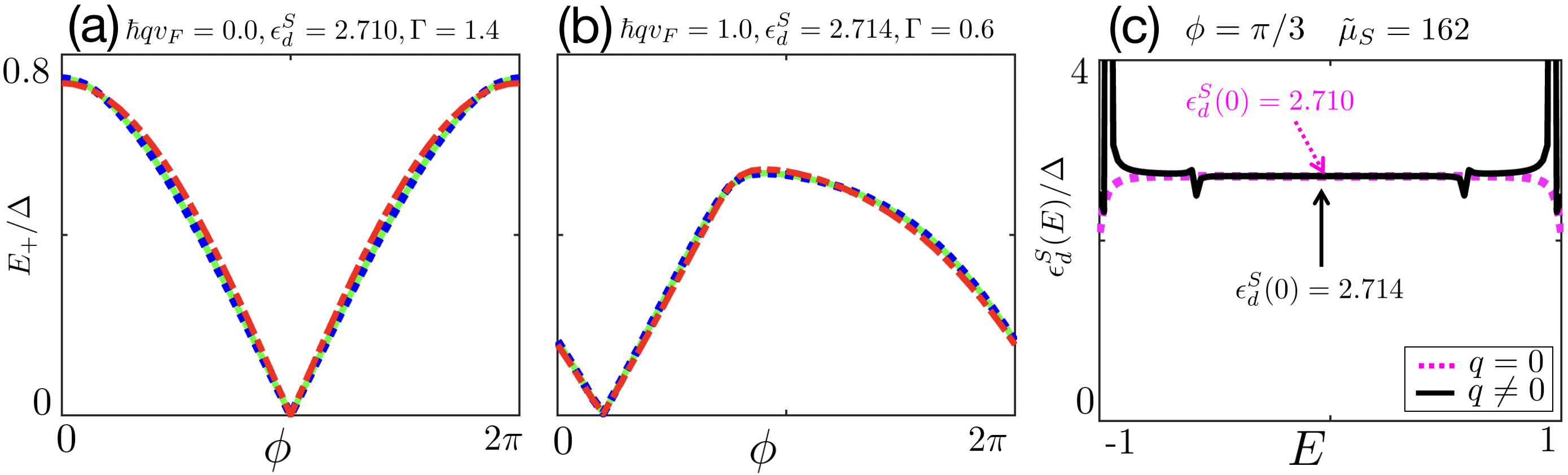
For , the -dependent additional phase difference results in the asymmetric dispersion [Fig. 2 (a) in the main text] thus giving rise to the superconducting diode effect [see Fig. 2 (c) in the main text]. To see how the asymmetric -dependence of the additional phase difference gives rise to asymmetric dispersions, let us consider the weak tunneling and low energy case () for simplicity in which we assume i) ) is independent of the inside the finite-momentum superconductor gap [Fig. 12 (c)], ii) , and iii) that eliminate the -dependence of the renormalization effects in both effective pair potential and Andreev level. Equation (115) then reduces to , which is plotted by the red lines of Fig. 12 (b). Numerically, we can obtain the exact -dependence of via the diagonalization of the BdG Hamiltonian (47). To calculate the additional phase difference for each phase difference , we have to substitute , , and into Eqs. (98) and (99) and then determine the additional phase shifts of the Andreev reflections in the left and right superconductors, i.e., and . We find that the additional phase difference is an asymmetric function of for [see Fig. 1 (c) in the main text] and therefore we obtain asymmetric dispersions with respect to , i.e., (see Fig. 12). Our fitting agrees with the results obtained from the numerical diagonalization of the BDG Hamiltonian (47).
Appendix F Ground state Fermion parity changes
In this section, we derive a condition for the ground-state fermion parity changes in our system in the presence of both Zeeman fields and . We discuss the cases with and without SO interaction.
F.1 Zero SO interaction () and ,
Here the secular equation (94) for the Andreev states in the dot reads
| (141) | ||||
The above equation can be obtained from Eq. (E.2) by a replacement () in the quantum dot (superconducting leads). The function renormalizes both Andreev levels and its spin splitting. Thus, Eq. (141) reduces to
| (142) | ||||
with
| (143) |
| (144) |
Therefore, we have obtained a compact implicit equation from which we can easily obtain the Andreev levels explicitly by iterations
| (145) |
The fermion parity changes happen at and hence we obtain the condition for it to occur
| (146) |
where we have , , , and , where we remove the dependence because , , , and are even function of (Figs. 10 and 11). Equation (146) helps explain how fermion parity changes can modify the SDE in the absence of spin-orbit coupling, Fig. 2 in the main text.
F.2 Nonzero SO interaction () and ,
In the presence of spin-orbit interaction, spin-up and spin-down electrons mix via tunneling matrix [Eq. (58)]. Substituting the Green function (107) and the tunneling matrix (58) into the self-energy (D.1), we obtain
| (147) |
The normal contributions are given by
| (148) |
| (149) |
Then, the anomalous contributions are given by
| (150) |
Here we are interested in the zero energy Andreev bound state, . Then, Eqs. (F.2-F.2) reduce to
| (151) | ||||
| (152) | ||||
| (153) | ||||
where we have used the fact that , , , and are even function of . Then, we reach
| (154) |
| (155) |
| (156) |
Solving the reduced determinantal equation (94) at , we find
| (157) |
These are the phase values at which fermion parity changes occur for the case with spin-orbit interaction and Zeeman magnetic fields, Fig. 3 of the main text.
References
- Ando et al. [2020] F. Ando, Y. Miyasaka, T. Li, J. Ishizuka, T. Arakawa, Y. Shiota, T. Moriyama, Y. Yanase, and T. Ono, Nature 584, 373 (2020).
- Bauriedl et al. [2022] L. Bauriedl, C. Bäuml, L. Fuchs, C. Baumgartner, N. Paulik, J. M. Bauer, K.-Q. Lin, J. M. Lupton, T. Taniguchi, K. Watanabe, et al., Nat. Commun. 13, 1 (2022).
- Shin et al. [2021] J. Shin, S. Son, J. Yun, G. Park, K. Zhang, Y. J. Shin, J.-G. Park, and D. Kim, arXiv preprint arXiv:2111.05627 (2021).
- Bocquillon et al. [2017] E. Bocquillon, R. S. Deacon, J. Wiedenmann, P. Leubner, T. M. Klapwijk, C. Brüne, K. Ishibashi, H. Buhmann, and L. W. Molenkamp, Nat. Nanotechnol. 12, 137 (2017).
- Pal et al. [2022] B. Pal, A. Chakraborty, P. K. Sivakumar, M. Davydova, A. K. Gopi, A. K. Pandeya, J. A. Krieger, Y. Zhang, S. Ju, N. Yuan, et al., Nat. Phys. 18, 1228 (2022).
- Baumgartner et al. [2022] C. Baumgartner, L. Fuchs, A. Costa, S. Reinhardt, S. Gronin, G. C. Gardner, T. Lindemann, M. J. Manfra, P. E. Faria Junior, D. Kochan, et al., Nat. Nanotechnol. 17, 39 (2022).
- Wu et al. [2022] H. Wu, Y. Wang, Y. Xu, P. K. Sivakumar, C. Pasco, U. Filippozzi, S. S. Parkin, Y.-J. Zeng, T. McQueen, and M. N. Ali, Nature 604, 653 (2022).
- Turini et al. [2022] B. Turini, S. Salimian, M. Carrega, A. Iorio, E. Strambini, F. Giazotto, V. Zannier, L. Sorba, and S. Heun, Nano Lett. 22, 8502 (2022).
- Lin et al. [2022] J.-X. Lin, P. Siriviboon, H. D. Scammell, S. Liu, D. Rhodes, K. Watanabe, T. Taniguchi, J. Hone, M. S. Scheurer, and J. Li, Nat. Phys. 18, 1221 (2022).
- Scammell et al. [2022] H. D. Scammell, J. Li, and M. S. Scheurer, 2D Materials 9, 025027 (2022).
- Davydova et al. [2022] M. Davydova, S. Prembabu, and L. Fu, Sci. Adv. 8, eabo0309 (2022).
- Narita et al. [2022] H. Narita, J. Ishizuka, R. Kawarazaki, D. Kan, Y. Shiota, T. Moriyama, Y. Shimakawa, A. V. Ognev, A. S. Samardak, Y. Yanase, et al., Nat. Nanotechnol. 17, 823 (2022).
- Jiang et al. [2022] J. Jiang, M. Milošević, Y.-L. Wang, Z.-L. Xiao, F. Peeters, and Q.-H. Chen, Phys. Rev. Appl. 18, 034064 (2022).
- Daido et al. [2022] A. Daido, Y. Ikeda, and Y. Yanase, Phys. Rev. Lett. 128, 037001 (2022).
- Yuan and Fu [2022] N. F. Yuan and L. Fu, Proc. Natl. Acad. Sci. 119, e2119548119 (2022).
- Ilić and Bergeret [2022] S. Ilić and F. Bergeret, Phys. Rev. Lett. 128, 177001 (2022).
- He et al. [2022] J. J. He, Y. Tanaka, and N. Nagaosa, New J. Phys. 24, 053014 (2022).
- Legg et al. [2022] H. F. Legg, D. Loss, and J. Klinovaja, Phys. Rev. B 106, 104501 (2022).
- Zhang et al. [2022] Y. Zhang, Y. Gu, P. Li, J. Hu, and K. Jiang, Phys. Rev. X 12, 041013 (2022).
- Tanaka et al. [2022] Y. Tanaka, B. Lu, and N. Nagaosa, Phys. Rev. B 106, 214524 (2022).
- Jiang and Hu [2022] K. Jiang and J. Hu, Nat. Phys. 18, 1145 (2022).
- Fulde and Ferrell [1964] P. Fulde and R. A. Ferrell, Phys. Rev. 135, A550 (1964).
- Larkin and Ovchinnikov [1965] A. Larkin and Y. N. Ovchinnikov, Soviet Physics-JETP 20, 762 (1965).
- Casalbuoni and Nardulli [2004] R. Casalbuoni and G. Nardulli, Rev. Mod. Phys. 76, 263 (2004).
- Bowers and Rajagopal [2002] J. A. Bowers and K. Rajagopal, Phys. Rev. D 66, 065002 (2002).
- Kenzelmann et al. [2008] M. Kenzelmann, T. Strassle, C. Niedermayer, M. Sigrist, B. Padmanabhan, M. Zolliker, A. Bianchi, R. Movshovich, E. D. Bauer, J. L. Sarrao, et al., Science 321, 1652 (2008).
- Mayaffre et al. [2014] H. Mayaffre, S. Krämer, M. Horvatić, C. Berthier, K. Miyagawa, K. Kanoda, and V. Mitrović, Nat. Phys. 10, 928 (2014).
- Kinjo et al. [2022] K. Kinjo, M. Manago, S. Kitagawa, Z. Mao, S. Yonezawa, Y. Maeno, and K. Ishida, Science 376, 397 (2022).
- Matsuda and Shimahara [2007] Y. Matsuda and H. Shimahara, Journal of the Physical Society of Japan 76, 051005 (2007).
- Kaur et al. [2005] R. Kaur, D. Agterberg, and M. Sigrist, Phys. Rev. Lett. 94, 137002 (2005).
- Sigrist et al. [2007] M. Sigrist, D. Agterberg, P. Frigeri, N. Hayashi, R. Kaur, A. Koga, I. Milat, K. Wakabayashi, and Y. Yanase, J. Magn. Magn. Mater. 310, 536 (2007).
- Agterberg and Kaur [2007] D. Agterberg and R. Kaur, Phys. Rev. B 75, 064511 (2007).
- Chen et al. [2018] A. Q. Chen, M. J. Park, S. T. Gill, Y. Xiao, D. Reig-i Plessis, G. J. MacDougall, M. J. Gilbert, and N. Mason, Nat. Commun. 9, 1 (2018).
- Wu et al. [2013] F. Wu, G.-C. Guo, W. Zhang, and W. Yi, Phys. Rev. Lett. 110, 110401 (2013).
- Hart et al. [2017] S. Hart, H. Ren, M. Kosowsky, G. Ben-Shach, P. Leubner, C. Brüne, H. Buhmann, L. W. Molenkamp, B. I. Halperin, and A. Yacoby, Nat. Phys. 13, 87 (2017).
- Zhang and Yi [2013] W. Zhang and W. Yi, Nat. Commun. 4, 1 (2013).
- Chan and Gong [2014] C. F. Chan and M. Gong, Phys. Rev. B 89, 174501 (2014).
- Dimitrova and Feigel’Man [2007] O. Dimitrova and M. Feigel’Man, Phys. Rev. B 76, 014522 (2007).
- Yuan and Fu [2021] N. F. Yuan and L. Fu, Proc. Natl. Acad. Sci. 118, e2019063118 (2021).
- Yuan and Fu [2018] N. F. Yuan and L. Fu, Phys. Rev. B 97, 115139 (2018).
- Levine [1965] J. L. Levine, Phys. Rev. Lett. 15, 154 (1965).
- Hansen [1969] O. Hansen, Phys. Rev. 181, 671 (1969).
- Bardeen [1962] J. Bardeen, Reviews of modern physics 34, 667 (1962).
- Zhu et al. [2021] Z. Zhu, M. Papaj, X.-A. Nie, H.-K. Xu, Y.-S. Gu, X. Yang, D. Guan, S. Wang, Y. Li, C. Liu, et al., Science 374, 1381 (2021).
- Dartiailh et al. [2021] M. C. Dartiailh, W. Mayer, J. Yuan, K. S. Wickramasinghe, A. Matos-Abiague, I. Žutić, and J. Shabani, Phys. Rev. Lett. 126, 036802 (2021).
- Bernevig [2013] B. A. Bernevig, in Topological Insulators and Topological Superconductors (Princeton university press, 2013).
- [47] Supplementary Materials , for detailed derivations of Eqs. (5) and (6), as well as the Andreev reflection in finite momentum superconductors which includes Refs. [45, 68, 39, 11, 44, 69, 22, 41, 42, 43, 46, 71, 72, 62, 63, 64, 65, 66, 67, 56, 6].
- Anderson [1964] P. Anderson, Acad. Press., NY 113 (1964).
- Bagwell [1992] P. F. Bagwell, Phys. Rev. B 46, 12573 (1992).
- Riedel and Bagwell [1998] R. A. Riedel and P. F. Bagwell, Phys. Rev. B 57, 6084 (1998).
- Beenakker [1991] C. Beenakker, Phys. Rev. Lett. 67, 3836 (1991).
- Beenakker et al. [2013] C. Beenakker, D. Pikulin, T. Hyart, H. Schomerus, and J. Dahlhaus, Phys. Rev. Lett. 110, 017003 (2013).
- Bardeen et al. [1969] J. Bardeen, R. Kümmel, A. Jacobs, and L. Tewordt, Phys. Rev. 187, 556 (1969).
- Chtchelkatchev and Nazarov [2003] N. M. Chtchelkatchev and Y. V. Nazarov, Phys. Rev. Lett. 90, 226806 (2003).
- Zhang and et al. [shed] X. Zhang and et al., (to be published).
- Silvester [2000] J. R. Silvester, Math. Gaz. 84, 460 (2000).
- Dell’Anna et al. [2007] L. Dell’Anna, A. Zazunov, R. Egger, and T. Martin, Phys. Rev. B 75, 085305 (2007).
- Hoffman et al. [2017] S. Hoffman, D. Chevallier, D. Loss, and J. Klinovaja, Phys. Rev. B 96, 1 (2017), arXiv:1705.03002 .
- Padurariu and Nazarov [2010] C. Padurariu and Y. V. Nazarov, Phys. Rev. B 81, 144519 (2010).
- González Rosado et al. [2021] L. González Rosado, F. Hassler, and G. Catelani, Phys. Rev. B 103, 035430 (2021).
- Spethmann et al. [2022] M. Spethmann, X.-P. Zhang, J. Klinovaja, and D. Loss, Phys. Rev. B 106, 115411 (2022).
- Meng et al. [2009] T. Meng, S. Florens, and P. Simon, Phys. Rev. B 79, 224521 (2009).
- Kurilovich et al. [2021] P. D. Kurilovich, V. D. Kurilovich, V. Fatemi, M. H. Devoret, and L. I. Glazman, Phys. Rev. B 104, 174517 (2021).
- Rozhkov and Arovas [1999] A. Rozhkov and D. P. Arovas, Phys. Rev. Lett. 82, 2788 (1999).
- Bauer et al. [2007] J. Bauer, A. Oguri, and A. Hewson, J. Phys. Condens. Matter 19, 486211 (2007).
- Meden [2019] V. Meden, J. Phys. Condens. Matter 31, 163001 (2019).
- Fatemi et al. [2021] V. Fatemi, P. Kurilovich, M. Hays, D. Bouman, T. Connolly, S. Diamond, N. Frattini, V. Kurilovich, P. Krogstrup, J. Nygard, et al., arXiv:2112.05624 (2021).
- Degtyarev et al. [2017] V. Degtyarev, S. Khazanova, and N. Demarina, Sci. Rep. 7, 3411 (2017).
- Banerjee et al. [2023] A. Banerjee, M. Geier, M. A. Rahman, C. Thomas, T. Wang, M. J. Manfra, K. Flensberg, and C. M. Marcus, arXiv:2301.01881 (2023), https://doi.org/10.48550/arXiv.2301.01881.
- Fletcher et al. [2007] J. Fletcher, A. Carrington, P. Diener, P. Rodiere, J.-P. Brison, R. Prozorov, T. Olheiser, and R. Giannetta, Phys. Rev. Lett. 98, 057003 (2007).
- Pillet et al. [2010] J. Pillet, C. Quay, P. Morfin, C. Bena, A. L. Yeyati, and P. Joyez, Nat. Phys. 6, 965 (2010).
- Pillet [2011] J.-D. Pillet, Tunneling spectroscopy of the Andreev bound states in a carbon nanotube, Ph.D. thesis, Université Pierre et Marie Curie-Paris VI (2011).