Queues with resetting: a perspective
Abstract
Performance modeling is a key issue in queuing theory and operation research. It is well-known that the length of a queue that awaits service or the time spent by a job in a queue depends not only on the service rate, but also crucially on the fluctuations in service time. The larger the fluctuations, the longer the delay becomes and hence, this is a major hindrance for the queue to operate efficiently. Various strategies have been adapted to prevent this drawback. In this perspective, we investigate the effects of one such novel strategy namely resetting or restart, an emerging concept in statistical physics and stochastic complex process, that was recently introduced to mitigate fluctuations-induced delays in queues. In particular, we show that a service resetting mechanism accompanied with an overhead time can remarkably shorten the average queue lengths and waiting times. We examine various resetting strategies and further shed light on the intricate role of the overhead times to the queuing performance. Our analysis opens up future avenues in operation research where resetting-based strategies can be universally promising.
1 Introduction
Queuing theory is usually considered to be a branch of operations research that mathematically studies the formation, function and other aspects of waiting lines that stretch in front of a service station [1, 2, 3, 4]. Queues are ubiquitous in nature and they appear in a wide range of applications ranging from supermarkets, banks, call-centers [5, 6], telecommunications [7, 8], airplane boarding [9, 10, 11], computer systems [12, 13], emergency services, transport phenomena[14, 15, 16] to gene expression [17, 18, 19, 20, 21] enzymatic and metabolic pathways [22, 23, 24, 25, 26]. Each set-up of a queue has its unique working principle. For example, a teller in the bank or a supermarket may work more or less at a constant rate but this can not be said for the computer servers or living entities like genes or enzymes which may often display more fluctuations in service time [27, 28, 29, 30]. In fact, it is now a well-established fact that the efficiency of a queue depends not only on the rate of the server but it is also extremely sensitive to the stochastic fluctuations in service times. As a result, these fluctuations have profound consequences and quite often they render acute backlogs and delays in queues stalling the work-conditions [13].
There has been a persistent strive to tailor generic strategies that can control and mitigate the adverse effect caused by stochastic service time fluctuations in queues especially the ones that encounter heavy tailed workloads [31]. Various scheduling policies have been developed eg, small jobs are being served first by the server instead of first-come-first-serve. Although this policy can be proven optimal under certain conditions, it is also criticized due to its lack of fairness [13]. Notably, these policies are applicable to queues where the source of service time fluctuations is rather extrinsic i.e, it depends on the variability in the job sizes or the numbers of items as in the supermarkets. However, these policies are not well-equipped to deal with situations where fluctuations in service times are intrinsic to the server itself. This is indeed the case for stochastic optimization algorithms, genes or the enzymes where stochastic fluctuations are intrinsic to the server [32, 33, 34]. Naturally, these policies turn out to be inadequate to be implemented for such scenarios and thus, novel approaches are very much in need.
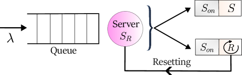
In a recent work [35], we proposed a novel approach, based on resetting or restart, to mitigate the problems caused by service time fluctuations in queuing systems. It was shown that the length of a queue can be significantly shortened by a simple service resetting policy. To understand the resetting mechanism, consider an arbitrary stochastic dynamical process which completes a task in some random time. However, the process can be restarted (i.e, started from scratch) intermittently before the completion of the task and thus it has to begin completely anew and repeat the same task [36, 37, 42, 45, 40, 44, 38, 43, 39, 41, 46, 47, 48]. This procedure repeats itself until the process reaches completion. The completion time will thus depend on the details of the underlying process and the resetting protocol. In a similar vein, consider a single server queue where the server has a task of completing one job at a time. This completion takes a random time – moreover, the source of stochastic fluctuations is considered to be intrinsic. To implement resetting, imagine this server being stopped intermittently and then restarted – thus, jobs whose service has been reset are now assigned fresh service times.
At a first glance one might wonder why restarting from scratch can expedite the completion of a complex random process. Indeed, this has been a quest in statistical physics and stochastic process for the last decade where resetting has been shown to systematically eliminate errand trajectories and find alternative pathways that can be avoid potential obstacles [36, 37, 42, 45, 40, 44, 50, 49, 51, 52, 53, 54]. Unveiling new such trajectories can often fasten the completion in particular when the resetting-free underlying processes possess search time with large fluctuations. This particular observation is quite intriguing as it states that resetting can overturn the high uncertainty due to large fluctuations in the underlying search time, thus converting a drawback into a favorable advantage. No wonder, why such resetting based strategies have been proven to be extremely useful in a wide range of search processes spanning from stochastic optimization [55, 56, 57], first passage processes[58, 61, 59, 60, 62], home-based foraging [63], chemical reactions [64, 65], income dynamics [66, 67] to transport over the last few years.
The goal of this perspective is to first introduce the topics “queues” and “resetting”, review the formulation of a single-server queue with instantaneous service resetting and to bring new insights when the service resetting is not instantaneous but involves an overhead or buffer time. We will discuss the ramifications of this overhead time and its interplay with the service time on the length of the queue or the waiting time. A pedagogic approach has been taken keeping the non-expert readers in mind.
The rest of the paper is structured in the following way. In Sec. 2 “Preliminaries”, we provide a brief overview of the M/G/1 queuing system with general service and Markovian job arrival – this will serve as the prototype model of a queue in this paper. We discuss the Pollaczek-Khinchin formula which gives an estimation of the mean number of jobs in the steady state of the M/G/1 queue, emphasizing the dependency of the latter to the service time variability. In Sec. 3 “Service with resetting”, we formulate the M/G/1 queuing model with service resetting where we associate a refractory time to the overall process. In effect, this ‘modified’ queue is similar to the standard queue with a compounded service time that depends on the resetting and overhead time. With this mapping, we can immediately use the Pollaczek-Khinchin formula in the M/G/1 queue with a modified service time to compute the mean number of jobs. In Sec. 4 “M/G/1 Queues with Poissonian service resetting”, we discuss the effects of Poissonian service resetting (i.e., resetting with a constant rate) on the mean number of jobs in the queue where the calculations simplify in multi-fold. In Sec. 5 “Service at an optimal resetting rate”, we study the mean number of jobs when the service is restarted at an optimal resetting rate under Poissonian resetting. We move on to demonstrate how resetting can reduce the number of jobs depending on the variability of the overhead time. In Sec. 6 “Application”, we illustrate how the general formalism developed so far can be used for the log-normal service time distribution and overhead times with different variability. We conclude in Sec. 7 “Discussion and Summary” with a summary and future perspective. Appendices provide detailed derivations and other technical results to keep the paper self-contained.
In what follows, we use the notations , , , and to denote, respectively, the probability density function, expectation, variance, Laplace transform and coefficient of variation of a non-negative random variable .
2 Preliminaries
Let us consider a single line queuing system where a server serves one job at a time and jobs await to be served in a first come first serve basis. Such a queue is often represented as M/G/1 queue in Kendall’s notation where the notation M stands for the Markovian or memory-less arrival of jobs. Here, we assume that the jobs arrive according to a Poisson process with rate and G stands for the service time of jobs, which can be drawn from a general distribution. We indicate this service time random variable as which is distributed according to . The last notation 1 simply indicates that one job should be served at a time. Notably, we assume that the server needs to wait some overhead time following a reset or a service. This is quite common in a computer software or algorithm where a buffer time is required to initialize and reload the program. Similar situations also appear in natural systems such as the chemical reaction or facilitated diffusion. We denote the overhead time by the random variable . Therefore, the total service time of the underlying process () is defined by the sum of and with the corresponding density . The service rate of this process can be defined as . Furthermore, one can define the utilization parameter that signifies the fraction of time the server works in steady state. To attain the steady state of the system the arrival rate of jobs must be less than the effective service rate so that . Otherwise, for , the number of jobs in the queue will blow up and the length of the queue will increase indefinitely.
The state space of the M/G/1 queue is denoted by the set , where the value of corresponds to the number of jobs in the queue, including the one being served. This number fluctuates in time as the arrival and service are random processes. One key observable in the queuing theory is the mean number of jobs in the system (queue+server) which is given by the famous Pollaczek-Khinchin formula in the steady state [13].
| (1) |
where is the utilization and
| (2) |
is the squared coefficient of variation or the variability in total service time of the underlying process. Several comments can be made here. First, note that the mean number of jobs increases monotonically as a function of the utilization and it diverges as leading to “piling up” of jobs. Secondly, is found to be highly sensitive to the variability in the service time. Namely, if , the second term on the RHS in Eq. (1) becomes negative leading to shorter queues. On the other hand, if the service time has large fluctuations namely , the second term adds positive contribution to leading to longer queues. It is thus evident that service time fluctuations are central to the behavior of the M/G/1 queue, and their effect in other queuing systems can also be anticipated in a similar way.
The mean waiting time of a job in the queue, i.e., the time elapsed from arrival to the end of service, is proportional to via Little’s law [13]. This results in
| (3) |
which again crucially depends on fluctuations in service time similar to the mean number of jobs. The fluctuations in service time can both be intrinsic and extrinsic to the server. If a server serves jobs of different sizes with constant rate, then the service time is extrinsic to the server and it will be dictated by the job size. As in supermarkets, the service time for the customers at the billing counter is determined by the number of items each customer buys. On the other hand, the fluctuation in the service time can also be intrinsic to the server itself. The catalytic reaction can be an example of this where to catalyze chemical reaction an enzyme takes different time between turnover cycle though the substrate and product molecule are chemically identical. We refer to [35] for a detailed discussion on the origin of service time fluctuations in queues.
3 Service with resetting
When service time fluctuations are intrinsic to the server in a queue, a service resetting can be implemented in the following way. Again we recall the M/G/1 queue where the jobs are being served one at a time. Consider the server that starts at time zero and, if allowed to take place without interruptions, completes after a random time . The service, however, is restarted at some random time following which service renews. Denoting the random service time of the compound process by it can be seen that
| (4) |
where is a random time drawn from a general distribution which accounts for the time delay that may occur prior to either service completion or resetting and is an independent and identically distributed copy of . To understand this equation, observe that when service occurs before restart, . However, if service is restarted at a time , then a new service time is drawn, and service restarts following the overhead time . In that case, we simply have . Thus, it can be seen that Eq. (4) forms a renewal structure. As shown in [35], here the service mechanism can be understood as a first passage process which is intermittently subjected to the resetting strategy. A comprehensive framework for first passage under resetting was developed in [68, 40]. We review this method partially in the (A) and only present the key results here. To this end, note that Eq. (4) can be recast in the following way
| (5) |
where is the minimum of and and is an indicator random variable which takes the value one when and zero otherwise. Eq. (5) can be used to compute the moment generating function of which we keep to the Appendix. The first and second moments however can be computed directly by taking expectations on both sides of Eq. (5). Performing the averages, one finds
| (6) | ||||
| (7) |
where is the probability of service being completed prior to restart, and stands for the conditional restart time given that restart occurred prior to service. Finally, recall that the variance in the service time is given by . Given the distribution of the resetting times and service times, it is straightforward task to compute both the moments in Eq. (6) and Eq. (7), as we will show explicitly in the next section.
4 M/G/1 Queues with Poissonian service resetting
There are numerous possible ways in which service and resetting mechanisms can mix and match. One such resetting mechanism namely the Poissonian resetting has been extensively studied in the recent past [36, 37, 58, 69, 68, 40, 61, 59, 46, 38, 41]. As the name suggests, here the number of resetting events in a given time interval is distributed according to the Poisson distribution. More on the technical ground, if the resetting occurs at a rate , the mean number of resetting events in time is given by and the resetting time is drawn from an exponential distribution i.e., . The mean and second moment of the service time can then be derived using Eq.s (6) and (7) (see (B) for the derivation)
| (8) | ||||
| (9) |
where is the Laplace transform of the service time , evaluated at the restart rate . The utilization of this queue is then given by , and the squared coefficient of variation of the service time is .
Under resetting mechanism, one notices that the queue service time is now modified to . Henceforth, one can replace with , and with , in Eq. (1) to compute the mean queue length under resetting. This yields
| (10) |
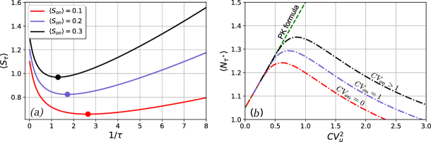
Similarly, the mean waiting time in the system can be derived from Little’s law [70, 13], yielding an analogous result to Eq. (3). To demonstrate the effect of resetting in a M/G/1 queue in the presence of a overhead time, we consider Fig. 2(a) as an illustrative example (details will be discussed in Sec. 6). Commencing from a service time distribution, service resetting has been introduced and the mean service time is plotted against the resetting rate for various overhead time distribution. We note that initially decreases, obtaining a minima at an optimal resetting rate before increasing further, as evident from the figure. The emergence of the optimal resetting rate is quite noteworthy as resetting does not only lower the mean service time but also renders a global minimum time. The next section is dedicated to a detailed analysis of and how it is connected to the generic service and overhead time.
5 Service at an optimal resetting rate
The optimal resetting rate that minimizes the mean service time can be obtained by setting
| (11) |
Substituting the expression for from equation (8) into Eq. (11), we find
| (12) |
where refers to the derivative of as a function of . Using from the above expression in Eq. (9) for the second moment , and simplifying further one arrives at the following relation for the variability of an optimally restarted process [68]
| (13) |
where is the variability of the overhead time and furthermore we have rewritten in terms of the -metrics in the following way
| (14) |
The relation in Eq. (13) is completely universal since it does not depend on the specific choice of the underlying service time and the overhead time. Our next goal is to understand how the mean queue length in Pollaczek-Khinchin formula would change with optimal resetting.
The mean length of the queue for the optimally restarted process is then given by the Pollaczek-Khinchin formula in Eq. (10) with the substitution . This results in
| (15) |
Now we can use the universal relation (13) for the optimally restarted process in above to find
| (16) |
where we have also used the fact that . Eq. (16) suggests that the mean queue length depends crucially on the variability of the overhead time. In the following section, we identify a few such different cases based on .
So far in the analysis, we have assumed that there exists a finite optimal resetting rate. But it is worthwhile to ask under what conditions this is guaranteed. Skipping details of the proof from C, we note that the general criteria that ensures the existence of an optimal reads
| (17) |
which again crucially depends on .
5.1 Resetting with no overhead
We first recap the scenario when there is no overhead time in the system. Thus, the service restarts immediately. This was well studied in [35]. In this case, and thus Eq. (8) and 9 simply reduce to [35]
| (18) | ||||
| (19) |
Moreover, the universal relation (13) simply becomes . As a result, the mean queue length turns out to be
| (20) |
which satisfies the following inequality . Thus, the mean number of jobs in the queue can be reduced by resetting service at an optimal rate. Moreover, the criterion for a finite reduces to . We refer to [35] for more details.
5.2 Overhead time with
We now consider a scenario when the overhead times are sampled from a distribution which is narrowly dispersed i.e., . Denoting the queue length by , one finds
| (21) |
where the second term in the above equation gives a negative contribution so that . The general condition in Eq. (17) suggests that for the case , one should have . This is a sufficient (but not necessary) condition that guarantees that a finite should exist.
Now, if a non-zero finite exists, we should have which essentially implies where recall and . Finally, noting that is a monotonically increasing function of , it becomes explicit that . Collecting all the pieces together we arrive at the following hierarchical inequality
| (22) |
which will always holds as long as and thus service resetting will certainly help to alleviate the queue. Since the criterion is not a necessary one, a finite optimal resetting rate may exist (resulting in a reduction in the queue length) even before (see C.1 for additional discussion). This analysis effectively shows that service resetting can reduce the mean queue length even in the presence of finite overhead times.
5.3 Overhead time with
Next, we turn our attention to the marginal case when . In this case, the second term in Eq. (16) vanishes and the mean queue length, denoted by , becomes
| (23) |
A simple manipulation then shows
| (24) |
where we have used the similar line of rationale as in the previous case and further argued that for the existence of a finite (see C.2 for additional discussion).
5.4 Overhead time with
Finally, we consider a scenario where the overhead times are drawn from a distribution which is broadly dispersed so that . In this case, we have
| (25) |
where the second term is strictly positive. However, in this case, condition does not guarantee as was done in the previous subsections. However, one can do a more careful analysis to show that there exists a sufficient (not necessary) condition that can reassure the inequality . This modified criterion reads (see C.3 for details)
| (26) |
Since is a control parameter in this problem, we can impose the above condition to see a reduction in the mean queue length under service resetting.
6 Application
To demonstrate the power of our approach, we consider a M/G/1 queue whose service times are distributed according to a log-normal distribution – a well-known service time distribution in the queuing literature [71, 72]. We will study the effect of resetting on this server for different overhead time distributions. We start with the following form of the log-normal distribution
| (27) |
for , where and . The mean and variance of the service time in this case are given by
| (28) | |||||
| (29) |
such that
| (30) |
which is independent of . In the previous sections, we have discussed the general results when the overhead time is drawn from some arbitrary distributions and furthermore illustrated the role of its variability . In what follows, we will focus on three representative cases with different but keeping fixed. Finally, we discuss the scenario when the latter condition is also relaxed.

6.1 Case I:
We start with the case when i.e., the overhead time distribution is sharply peaked around its mean so that . In this case, variability of the underlying process can be expressed as
| (31) |
In Fig. 2(a), we plot the mean service time as a function of resetting rate for different values of fixing and . A minimum of is obtained at an optimal resetting rate which varies with . Our next goal is to understand the behavior of mean queue length as a function of . To vary , we keep and fixed but modulate in Eq. (31). For each , we first optimize as a function of , compute the optimal resetting rate , and then plugin the mean service time and the variability at this optimality into Eq. (21). Note that the existence of an optimal resetting rate is not guaranteed for any as was discussed in Sec. (C.1). Clearly, for , one finds and thus the plots for the underlying and reset process overlap with each other. However, as becomes finite, we can clearly see a deviation from the underlying PK formula and one observes as pointed out in Sec. C.1. The bottom curve in Fig. 2(b) shows how the mean queue length dramatically goes down as one gradually increases .
6.2 Case II:
Next, we turn our attention to the case where is drawn from an exponential distribution, such that where is the rate parameter of the distribution. This implies and so that . Therefore, the of the underlying process can be expressed as
| (32) |
As before, we keep fixed at 0.5 and choose to be the control parameter to vary . Similar optimization procedure is followed to obtain for different and then is finally substituted into Eq. (23). For , we find . However, as we increase , a clear deviation i.e., is observed. Here, behaves as a sharp boundary where the transition occurs. The middle curve in Fig. 2(b) summarizes this behavior.
6.3 Case III:
Finally, to demonstrate the effect of resetting for , we consider the Weibull distribution , where is the shape parameter and is the scale parameter of the distribution. In this case, the mean and variance of the overhead time are given by
| (33) | |||
| (34) |
where is the Gamma function of order . If is set to , becomes and thus becomes independent of . The variability of the the underlying process can then be expressed as
| (35) |
We choose so that is fixed at . Performing the same optimization procedure, keeping and fixed, as done in the previous subsections, we can show when the condition (26) is satisfied. As also evident from Fig. 2(b), the deviation from the PK formula occurs only at a higher in this case.
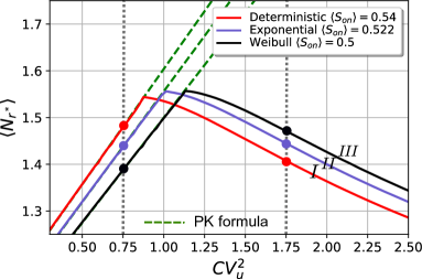
Thus, resetting has more pronounced effect on the queue that experiences larger fluctuations in the overhead time albeit having a smaller .
6.4 Mean queue length for different
So far we have assumed different while keeping fixed to estimate the mean queue length. Here, we relax this condition and study a combined effect when both of them are varied. Recall from the PK-formula that mean queue length increases linearly with when optimal resetting rate is fixed at zero so that . Similarly, for a fixed , one would expect that the length of the queue should be proportional to i.e., for a large overhead time, the queue will also be longer. For instance, take a fixed in Fig. 3 and vary . It is evident from the left vertical dashed line that the mean queue length increases with an increasing . The coloured circles represent the respective values of the queue length for the cases with different as shown in Fig. 3. Thus, here, one has
| (36) |
How can we compare between the queue lengths for different under optimal Poisson resetting? It turns out that the mean length of a queue with a higher can be reduced more dramatically with the introduction of resetting compared to an another queue with a lower if the former has a lower . This can be seen again from Fig. 3 as we set for which is non-zero and thus we are in the resetting-dominated regime. We can immediately note that the change in the order of the curves for namely
| (37) |
where the following order for the variability and the mean is maintained. In Fig. 3, we provide technical details that lead to this observation. While here we make this observation for the log-normal service time distribution, we believe that similar conclusions should hold for other service time distributions.
7 Discussion and Summary
Designing strategies that can optimize the number of jobs in a queue is an integral part of queuing theory. In particular, the key issue is to harness the large stochastic fluctuations in service times that can have deleterious effects in the performance of a queue. This has been alluded on various occasions in queuing theory in the context of computing workloads where the service time distributions have high variability. One such example arises in the UNIX process lifetime measurements [13, 73]. In this perspective article, we review an interesting recent development which aims to address performance improvement of systems with high-variability workloads (see [35, 74] and also [75]). We show that service resetting can be a useful strategy to mitigate these problems. In particular, we consider a M/G/1 queue system where the jobs arrive at a constant rate and the server has two components: its own service time accompanied by an overhead/buffer time. The service is intermittently subjected to resetting and we have studied the ramifications of resetting protocols on the performance of the queue. We develop a renewal theory for the service time under resetting with overhead time and show how the modified service can be incorporated into the famous Pollaczek-Khinchin formula that provides an estimation of the mean length of the mean number of jobs in the queue.
Our analysis unveils three possible scenarios for the overhead time distribution: narrowly dispersed, marginally dispersed and broadly dispersed. In all these cases, we show that an optimally engineered resetting mechanism can either match or outperform the efficiency of the queue than the one without resetting. Specifically, we have shown that resetting can dramatically reduce queue lengths when applied to servers that have high variability in the underlying service time. As such, resetting can alleviate the detrimental affect of large fluctuations by not only shortening the mean service time but also reducing the relative stochastic fluctuations around this mean, hence providing a two-fold advantage.
In the main text, we have only discussed the effects of Poissonian resetting. However, the general formalism developed therein can also be used to investigate other resetting strategy namely sharp or deterministic resetting [76, 40, 77]. Here, resetting is being conducted stroboscopically after a fixed time. This is strongly motivated from the earlier studies in the resetting community where sharp resetting has been proven to be a dominant strategy within the vast space of stochastic restart strategies irrespective of the underlying process that is being restarted. To see the effect of this resetting strategy, we first assume that the resetting occurs after every units of time so that
| (38) |
Using Eqs. (6) and (7), one can immediately obtain the the mean and the second moment of the service time under sharp resetting Eq. (D)
| (39) | ||||
| (40) |
where is the survival probability associated with the service. In simple words, it estimates the probability that the service has not occurred till time i.e., . For the log-normal service time as defined in Sec. 6, the survival probability can be computed
| (41) |
The mean queue length under sharp resetting can be obtained by substituting the metrics of the modified service time into Eq. (10)
| (42) |
where and is the variability of the service time under resetting. As before, we can find the optimal resetting time by setting . Combining with this optimal relation, we plot the mean queue length as a function of the underlying service time variability for different overhead time distributions in Fig. 4(b). It is seen that resetting can reduce the number of jobs in a queue regardless of the specific choice for .
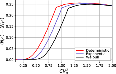
It is moreover interesting to compare the mean queue length under optimal Poisson and sharp resetting. To this end, we first recall from the theory of first passage under resetting that the mean completion time under optimal sharp resetting is always smaller or equal than that obtained under optimal Poissonian resetting. Here too, we find that the mean service time with overheads also respects the same relation (see Fig. 4(a)). Finally, we plot the difference between two optimally restarted queue lengths namely as a function of the underlying service time variability for overhead times with in Fig. 5. Quite remarkably, we find that this difference strictly stays positive which essentially implies that the mean number of jobs in the queue can be reduced further by resetting service at an optimal time rather than at an optimal rate. This observation is of practical importance since it reveals additional benefits in the performance modeling that can be gained by applying sharp resetting.
The formalism developed herein for the service time with overheads and resetting is not restricted to the M/G/1 queue, but in principle, can also be applied to other queues such as the G/G/1 queue where the arrivals are not necessarily Markovian [13]. Similar renewal methods can also be employed to analyze queues when the service time of the job has two components; one intrinsic component is the server slowdown and job’s inherent size being the other extrinsic component [74]. Similar to [35] and as shown here, resetting was shown to be a useful protocol to reduce the mean queue length. It will be interesting to study different trade-offs due to the overhead times in the above-mentioned queuing set-ups. There are many open frontiers with respect to the resetting based task assignment policies. Take for example a M/G/n queue that consists of a single queue but servers. When a server completes a job, it takes up the next job that is available at the head of the queue [13]. It is possible to apply resetting protocols independently to the individual servers as long as the ‘modified service’ is applied to the same job. However, in a more naturalistic scenario, it is possible that a fraction of servers needs to be reset simultaneously. This renders a correlated queuing system and one can not readily apply the formalism developed here. These possible extensions to multiserver queues, farms and networks are open for future research.
Concluding, we believe that this perspective has shed light on the feasibility of applying resetting based strategies to the queuing systems. Hopefully, this will bridge a gap between the queuing and the resetting community and also will encourage the researchers to attempt and design more resetting based solutions in queuing systems with potential applications to computer science, randomized numerical algorithms, and active living systems.
8 Acknowledgements
The numerical calculations reported in this work were carried out on the IMSc-1 cluster, which is maintained and supported by the Institute of Mathematical Science’s High-Performance Computing Center. RR gratefully acknowledges support from the IMSc Post-Doctoral Fellowship. AP acknowledges research support from the Department of Science and Technology, India, SERB Start-up Research Grant Number SRG/2022/000080 and Department of Atomic Energy, Government of India.
Appendix A Moment generating function of
In this section, we try to find the general expression for the mean and second moment as written in Eq. (6) and Eq. (7). For that we first find the general Laplace transform or the moment generating function of . Using that one can find all the moments in systematic fashion as we show below. We start by recalling Eq. (4) from the main text
| (43) |
The above equation can also be written in a more compact way as
| (44) |
where is the indicator function which takes the value 1 when and zero otherwise. Thus,
| (45) |
Let us now define as the moment generating function of the random variable , from which all its moments can be easily found. The Laplace transform of Eq. (44) can be given as
| (46) |
where and . We have also used the fact that is an independent and identically distributed copy of and thus independent of . Performing the expectations over the indicator functions, we find
| (47) |
from where one finds
| (48) |
This is an exact expression for the distribution of in Laplace space. This is also the moment generating function from which moment of can be computed directly via
| (49) |
For instance, the first moment reads
| (50) |
which is Eq. (6) with the identification . A similar exercise for the second moment gives
| (51) |
which is identified as the Eq. (7) in the main text. Eq. (49) thus encodes all the information about the higher moments.
Appendix B Moments of the service time for Poissonian resetting
In this section we take the representative case when the resetting times are drawn from an exponential distribution given by
| (52) |
where is the resetting rate. The cumulative function is given by
| (53) |
The distribution of the random variable can be computed by noting
| (54) |
from which one can gets
| (55) |
which can be used to compute all the moments for the random variable .
Mean service time with overheads: To compute the mean, we note that the first term on the numerator in Eq. (6)) can be written as
| (56) |
where . The denominator can be written as
| (57) |
For exponential resetting times and we have
| (58) |
Combining together, we find
| (59) |
which is Eq. (8) in main text.
Second moment of the service time with overheads: To find the second moment for Poisson resetting, we now use Eq. (7). The expectation in the numerator can be computed directly using Eq. (55)
| (60) |
In the above derivation we have used the following property . Next, to calculate we need to use the density of the conditional time which is given by
| (61) |
Then, can be expressed as
| (62) |
Substituting Eqs. (60) and (62) into Eq. (7), one obtains
| (63) |
which was announced in Eq. (9) in the main text.
Appendix C General discussion on the “resetting induced efficiency criterion” for the mean queue length with different variability
In this section, we elaborate more on the general conditions that were obtained in Sec. (5) to underpin the effect of resetting. We start by deriving the most general criterion that ensures the existence of an optimal . To see this, we introduce an infinitesimal resetting rate and ask under what condition the following inequality holds. Expanding Eq. (8) in the power of and imposing the above condition, we derive a universal relation
| (64) |
that guarantees the existence for an optimal resetting rate [45]. In terms of with the help of Eq. (14) this criterion takes the form
| (65) |
The above equation will be central to our remaining discussion where we study various cases for .
C.1 Case I:
In Eq. (22) in the main text we argued that for the mean queue length can be reduced by introducing resetting when . However, we emphasize that this is not a necessary (albeit sufficient) condition. From Eq. (65) we notice that the RHS is less than one for . This in turn implies a finite optimal value of also can be found under the same condition. This implies that becomes less than for . As a result, for a sufficiently small , one can still have from Eq. (21). In Fig. 3 we indeed find that the deviation occurs at value of which is less than unity.
C.2 Case II:
In this case the RHS of Eq. (65) becomes exactly unity and hence, a finite optimal shows up only when . It is thus evident from Eq. (24) that is both a necessary and sufficient condition for the reduction in the mean queue length. As shown in Fig. 3, the transition point (where ) is exactly found at .
C.3 Case III:
In this case the RHS of Eq. (65) is strictly greater than one. One can thus expect to find an optimal for values of . Thus the condition will be satisfied only when . This is also evident from Fig. 3 where we see that the transition point occurs at .
To derive the criterion (Eq. (26)) as mentioned in the main text we recall the PK formula from Eq. (25) for the optimally restarted process and the same without resetting from Eq. (1)
| (66) | ||||
| (67) |
and impose the condition . For a finite , this would yield
| (68) |
which gives the criterion obtained in Eq. (26) where we have substituted . Finally, we remark that this is a sufficient condition (but not necessary). In other words, one can still find a where this condition is not satisfied but the inequality holds.
Appendix D Moments for sharp resetting times
This section is dedicated to compute the first two moments of the service time under sharp resetting. Here, resetting occurs always after a fixed time interval such that
| (69) |
from which one can see
| (70) |
where is the Heaviside theta function which takes value unity only when and zero otherwise.
Mean service time with overheads: The numerator in Eq. (6) can be computed in the following way
| (71) |
where is the survival probability of the process up to time , which indicates the probability that the service has not yet been completed up to time . The denominator in Eq. (6) is found to be
| (72) |
Substituting Eq. (71) and Eq. (72) in Eq. (6) we obtain the first moment for sharp resetting as
| (73) |
which was announced in Eq. (39).
Second moment of service time with overheads: Following the same procedure as the previous section, we find
| (74) |
The quantity can also be obtained from Eq. (61) directly
| (75) |
Using Eqs. (74) and (75) in Eq. (7), we arrive at the following expression for the second moment of service time with overheads
| (76) |
which is Eq. (40) in the main text.
References
References
- [1] Adan, I., and Jacques R., 2002. Queueing theory. Eindhoven University of Technology. Department of Mathematics and Computing Science. p.104-106.
- [2] Cohen, J.W., 2012. The single server queue. Elsevier.
- [3] Haviv, M., 2013. Queues. New York: Springer.
- [4] Newell, C., 2013. Applications of queueing theory (Vol. 4). Springer Science & Business Media.
- [5] Gans, N., Koole, G. and Mandelbaum, A., 2003. Telephone call centers: Tutorial, review, and research prospects. Manufacturing & Service Operations Management, 5(2), pp.79-141.
- [6] Koole, G. and Mandelbaum, A., 2002. Queueing models of call centers: An introduction. Annals of Operations Research, 113(1), pp.41-59.
- [7] Daigle, J.N., 2005. Queueing theory with applications to packet telecommunication. Springer Science & Business Media.
- [8] Lakatos, L., Szeidl, L. and Telek, M., 2013. Introduction to queueing systems with telecommunication applications (Vol. 388). New York: Springer.
- [9] Bachmat, E., Berend, D., Sapir, L., Skiena, S. and Stolyarov, N., 2009. Analysis of airplane boarding times. Operations Research, 57(2), pp.499-513.
- [10] Bachmat, E., 2019. Airplane boarding meets express line queues. European Journal of Operational Research, 275(3), pp.1165-1177.
- [11] Erland, S., Kaupužs, J., Frette, V., Pugatch, R. and Bachmat, E., 2019. Lorentzian-geometry-based analysis of airplane boarding policies highlights “slow passengers first” as better. Physical Review E, 100(6), p.062313.
- [12] Cooper, R.B., 1981, January. Queueing theory. In Proceedings of the ACM’81 conference (pp. 119-122).
- [13] Harchol-Balter, M., 2013. Performance modeling and design of computer systems: queueing theory in action. Cambridge University Press.
- [14] Helbing, D., 2001. Traffic and related self-driven many-particle systems. Reviews of modern physics, 73(4), p.1067.
- [15] Averin, D.V., 2005. Electrons held in a queue. Nature, 434(7031), pp.285-287.
- [16] Romano, M.C., Thiel, M., Stansfield, I. and Grebogi, C., 2009. Queueing phase transition: theory of translation. Physical review letters, 102(19), p.198104.
- [17] Arazi, A., Ben-Jacob, E. and Yechiali, U., 2004. Bridging genetic networks and queueing theory. Physica A: Statistical Mechanics and its Applications, 332, pp.585-616.
- [18] Gelenbe, E., 2007. Steady-state solution of probabilistic gene regulatory networks. Physical Review E, 76(3), p.031903.
- [19] Jia, T. and Kulkarni, R.V., 2011. Intrinsic noise in stochastic models of gene expression with molecular memory and bursting. Physical review letters, 106(5), p.058102.
- [20] Kumar, N., Singh, A. and Kulkarni, R.V., 2015. Transcriptional bursting in gene expression: analytical results for general stochastic models. PLoS computational biology, 11(10), p.e1004292.
- [21] Jun, S., Si, F., Pugatch, R. and Scott, M., 2018. Fundamental principles in bacterial physiology—history, recent progress, and the future with focus on cell size control: a review. Reports on Progress in Physics, 81(5), p.056601.
- [22] Mather, W.H., Cookson, N.A., Hasty, J., Tsimring, L.S. and Williams, R.J., 2010. Correlation resonance generated by coupled enzymatic processing. Biophysical journal, 99(10), pp.3172-3181.
- [23] Cookson, N.A., Mather, W.H., Danino, T., Mondragón‐Palomino, O., Williams, R.J., Tsimring, L.S. and Hasty, J., 2011. Queueing up for enzymatic processing: correlated signaling through coupled degradation. Molecular systems biology, 7(1), p.561.
- [24] Mather, W.H., Hasty, J., Tsimring, L.S. and Williams, R.J., 2011. Factorized time-dependent distributions for certain multiclass queueing networks and an application to enzymatic processing networks. Queueing systems, 69(3), pp.313-328.
- [25] Evstigneev, V.P., Holyavka, M.G., Khrapatiy, S.V. and Evstigneev, M.P., 2014. Theoretical description of metabolism using queueing theory. Bulletin of mathematical biology, 76(9), pp.2238-2248.
- [26] Kloska, S., Pałczyński, K., Marciniak, T., Talaśka, T., Nitz, M., Wysocki, B.J., Davis, P. and Wysocki, T.A., 2021. Queueing theory model of Krebs cycle. Bioinformatics.
- [27] Kou, S.C., Cherayil, B.J., Min, W., English, B.P. and Xie, X.S., 2005. Single-Molecule Michaelis- Menten Equations. The Journal of Physical Chemistry B, 41(109), pp.19068-19081.
- [28] Moffitt, J.R. and Bustamante, C., 2014. Extracting signal from noise: kinetic mechanisms from a Michaelis–Menten‐like expression for enzymatic fluctuations. The FEBS journal, 281(2), pp.498-517.
- [29] Moffitt, J.R., Chemla, Y.R. and Bustamante, C., 2010. Methods in statistical kinetics. Methods in enzymology, 475, pp.221-257.
- [30] Velonia, K., Flomenbom, O., Loos, D., Masuo, S., Cotlet, M., Engelborghs, Y., Hofkens, J., Rowan, A.E., Klafter, J., Nolte, R.J. and de Schryver, F.C., 2005. Single‐enzyme kinetics of CALB‐catalyzed hydrolysis. Angewandte Chemie, 117(4), pp.566-570.
- [31] Whitt, W., 2000. The impact of a heavy-tailed service-time distribution upon the M/GI/s waiting-time distribution. Queueing Systems, 36(1), pp.71-87.
- [32] Spall, J.C., 2005. Introduction to stochastic search and optimization: estimation, simulation, and control (Vol. 65). John Wiley & Sons.
- [33] English, B.P., Min, W., Van Oijen, A.M., Lee, K.T., Luo, G., Sun, H., Cherayil, B.J., Kou, S.C. and Xie, X.S., 2006. Ever-fluctuating single enzyme molecules: Michaelis-Menten equation revisited. Nature chemical biology, 2(2), pp.87-94.
- [34] Flomenbom, O., Velonia, K., Loos, D., Masuo, S., Cotlet, M., Engelborghs, Y., Hofkens, J., Rowan, A.E., Nolte, R.J., Van der Auweraer, M. and de Schryver, F.C., 2005. Stretched exponential decay and correlations in the catalytic activity of fluctuating single lipase molecules. Proceedings of the National Academy of Sciences, 102(7), pp.2368-2372.
- [35] Bonomo O. L., Pal A. and Reuveni S., 2022. Mitigating long queues and waiting times with service resetting. PNAS Nexus 1, pgac070.
- [36] Evans, M.R. and Majumdar, S.N., 2011. Diffusion with stochastic resetting. Physical review letters, 106(16), p.160601.
- [37] Evans, M.R. and Majumdar, S.N., 2011. Diffusion with optimal resetting. Journal of Physics A: Mathematical and Theoretical, 44(43), p.435001.
- [38] Chechkin, A. and Sokolov, I.M., 2018. Random search with resetting: a unified renewal approach. Physical review letters, 121(5), p.050601.
- [39] Montanari, A. and Zecchina, R., 2002. Optimizing searches via rare events. Physical review letters, 88(17), p.178701.
- [40] Pal, A. and Reuveni, S., 2017. First Passage under Restart. Physical review letters, 118(3), p.030603.
- [41] Pal, A., 2015. Diffusion in a potential landscape with stochastic resetting. Physical Review E, 91(1), p.012113.
- [42] Evans, M.R., Majumdar, S.N. and Schehr, G., 2020. Stochastic resetting and applications. Journal of Physics A: Mathematical and Theoretical, 53(19), p.193001.
- [43] Kumar, A. and Pal, A., 2023. Universal framework for record ages under restart. Physical Review Letters, 130(15), p.157101.
- [44] Pal, A., Eliazar, I. and Reuveni, S., 2019. First passage under restart with branching. Physical review letters, 122(2), p.020602.
- [45] Pal, A., Kostinski, S. and Reuveni, S., 2022. The inspection paradox in stochastic resetting. J. Phys. A: Math. Theor. 55 021001.
- [46] Tal-Friedman, O., Pal, A., Sekhon, A., Reuveni, S. and Roichman, Y., 2020. Experimental realization of diffusion with stochastic resetting. J. Phys. Chem. Lett. 2020, 11, 17, 7350–7355.
- [47] Besga, B., Bovon, A., Petrosyan, A., Majumdar, S.N. and Ciliberto, S., 2020. Optimal mean first-passage time for a Brownian searcher subjected to resetting: experimental and theoretical results. Physical Review Research, 2(3), p.032029.
- [48] Paramanick, S., Pal, A., Soni, H. and Kumar, N., 2023. Programming tunable active dynamics in a self-propelled robot. arXiv preprint arXiv:2306.06609.
- [49] Evans, M.R. and Majumdar, S.N., 2018. Effects of refractory period on stochastic resetting. Journal of Physics A: Mathematical and Theoretical, 52(1), p.01LT01.
- [50] Pal, A., Stojkoski, V. and Sandev, T., 2023. Random resetting in search problems. arXiv preprint arXiv:2310.12057. To appear in the book ‘THE TARGET PROBLEM’ (Eds. D. S. Grebenkov, R. Metzler, G. Oshanin)
- [51] Sar, G.K., Ray, A., Ghosh, D., Hens, C. and Pal, A., 2023. Resetting-mediated navigation of an active Brownian searcher in a homogeneous topography. Soft Matter, 19(24), pp.4502-4518.
- [52] Ray, A., Pal, A., Ghosh, D., Dana, S.K. and Hens, C., 2021. Mitigating long transient time in deterministic systems by resetting. Chaos: An Interdisciplinary Journal of Nonlinear Science, 31(1).
- [53] Jain, S., Boyer, D., Pal, A. and Dagdug, L., 2023. Fick–Jacobs description and first passage dynamics for diffusion in a channel under stochastic resetting. The Journal of Chemical Physics, 158(5).
- [54] Sandev, T., Domazetoski, V., Kocarev, L., Metzler, R. and Chechkin, A., 2022. Heterogeneous diffusion with stochastic resetting. Journal of Physics A: Mathematical and Theoretical, 55(7), p.074003.
- [55] Luby, M., Sinclair, A. and Zuckerman, D., 1993. Optimal speedup of Las Vegas algorithms. Information Processing Letters, 47(4), pp.173-180.
- [56] Thrasher, W. J. and Mascagni, M., 2020. Examining sharp restart in a Monte Carlo method for the linearized Poisson–Boltzmann equation Monte Carlo Methods Appl. 26 223–44
- [57] Blumer, O., Reuveni, S. and Hirshberg, B., 2022. Stochastic resetting for enhanced sampling. The journal of physical chemistry letters, 13(48), pp.11230-11236.
- [58] Kusmierz, L., Majumdar, S.N., Sabhapandit, S. and Schehr, G., 2014. First order transition for the optimal search time of Lévy flights with resetting. Physical review letters, 113(22), p.220602.
- [59] Ahmad, S., Nayak, I., Bansal, A., Nandi, A. and Das, D., 2019. First passage of a particle in a potential under stochastic resetting: A vanishing transition of optimal resetting rate. Physical Review E, 99(2), p.022130.
- [60] Campos, Daniel. and Méndez, Vicenc., 2015. Phase transitions in optimal search times: How random walkers should combine resetting and flight scales. Physical Review E, 92(6), p.062115.
- [61] Pal, A. and Prasad, V.V., 2019. First passage under stochastic resetting in an interval. Physical Review E, 99(3), p.032123.
- [62] Yin, R. and Barkai, E., 2023. Restart expedites quantum walk hitting times. Physical Review Letters, 130(5), p.050802.
- [63] Pal, A., Kuśmierz, Ł. and Reuveni, S., 2020. Search with home returns provides advantage under high uncertainty. Physical Review Research, 2(4), p.043174.
- [64] Reuveni, S., Urbakh, M. and Klafter, J., 2014. Role of substrate unbinding in Michaelis–Menten enzymatic reactions. Proceedings of the National Academy of Sciences, 111(12), pp.4391-4396.
- [65] Biswas, A., Pal, A., Mondal, D. and Ray, S., 2023. Rate enhancement of gated drift-diffusion process by optimal resetting. The Journal of Chemical Physics, 159(5).
- [66] Stojkoski, V., Jolakoski, P., Pal, A., Sandev, T., Kocarev, L. and Metzler, R., 2022. Income inequality and mobility in geometric Brownian motion with stochastic resetting: theoretical results and empirical evidence of non-ergodicity. Philosophical Transactions of the Royal Society A, 380(2224), p.20210157.
- [67] Jolakoski, P., Pal, A., Sandev, T., Kocarev, L., Metzler, R. and Stojkoski, V., 2023. A first passage under resetting approach to income dynamics. Chaos, Solitons & Fractals, 175, p.113921.
- [68] Reuveni, S., 2016. Optimal stochastic restart renders fluctuations in first passage times universal. Physical review letters, 116(17), p.170601.
- [69] Kuśmierz, Ł. and Gudowska-Nowak, E., 2015. Optimal first-arrival times in Lévy flights with resetting. Physical Review E, 92(5), p.052127.
- [70] Nelson, R., 2013. Probability, stochastic processes, and queueing theory: the mathematics of computer performance modeling. Springer Science & Business Media.
- [71] Brown, L., Gans, N., Mandelbaum, A., Sakov, A., Shen, H., Zeltyn, S. and Zhao, L., 2005. Statistical analysis of a telephone call center: A queueing-science perspective. Journal of the American statistical association, 100(469), pp.36-50.
- [72] Gualandi, S. and Toscani, G., 2018. Call center service times are lognormal: A Fokker–Planck description. Mathematical Models and Methods in Applied Sciences, 28(08), pp.1513-1527.
- [73] Harchol-Balter, M., 2000, April. Task assignment with unknown duration. In Proceedings 20th IEEE International Conference on Distributed Computing Systems (pp. 214-224). IEEE.
- [74] Bonomo, O.L., Yechiali, U., and Reuveni, S., 2021. Queues with service resetting, arxiv preprint :2311.07770.
- [75] Bressloff, P.C., 2020. Queueing theory of search processes with stochastic resetting. Physical Review E, 102(3), p.032109.
- [76] Pal, A., Kundu, A. and Evans, M.R., 2016. Diffusion under time-dependent resetting. Journal of Physics A: Mathematical and Theoretical, 49(22), p.225001.
- [77] Bhat, U., De Bacco, C. and Redner, S., 2016. Stochastic search with Poisson and deterministic resetting. Journal of Statistical Mechanics: Theory and Experiment, 2016(8), p.083401.
- [78] Redner, S., 2001. A guide to first-passage processes. Cambridge university press.
- [79] Luby, M., Sinclair, A. and Zuckerman, D., 1993. Optimal speedup of Las Vegas algorithms. Information Processing Letters, 47(4), pp.173-180.
- [80] Gomes, C.P., Selman, B. and Kautz, H., 1998. Boosting combinatorial search through randomization. AAAI/IAAI, 98, pp.431-437.
- [81] Jackson, R.R.P., 1954. Queueing systems with phase type service. Journal of the Operational Research Society, 5(4), pp.109-120.
- [82] Askin, R.G., and Standridge, C.R. 1993. Modeling and analysis of manufacturing systems. John Wiley & Sons Incorporated.
- [83] Kendall, D.G., 1953. Stochastic processes occurring in the theory of queues and their analysis by the method of the imbedded Markov chain. The Annals of Mathematical Statistics, pp.338-354.
- [84] Bonomo, O.L. and Pal, A., 2021. First passage under restart for discrete space and time: Application to one-dimensional confined lattice random walks. Physical Review E, 103(5), p.052129.
- [85] Crovella, M.E. and Bestavros, A., 1996, May. Self-similarity in World Wide Web traffic: Evidence and possible causes. In Proceedings of the 1996 ACM SIGMETRICS international conference on Measurement and modeling of computer systems (pp. 160-169).
- [86] Barford, P. and Crovella, M., 1998, June. Generating representative web workloads for network and server performance evaluation. In Proceedings of the 1998 ACM SIGMETRICS joint international conference on Measurement and modeling of computer systems (pp. 151-160).
- [87] Crovella, M.E., Taqqu, M.S. and Bestavros, A., 1998. Heavy-tailed probability distributions in the World Wide Web. A practical guide to heavy tails, 1, pp.3-26.
- [88] Shaikh, A., Rexford, J. and Shin, K.G., 1999. Load-sensitive routing of long-lived IP flows. ACM SIGCOMM Computer Communication Review, 29(4), pp.215-226.
- [89] Kingman, J.F.C., 1961, October. The single server queue in heavy traffic. In Mathematical Proceedings of the Cambridge Philosophical Society (Vol. 57, No. 4, pp. 902-904). Cambridge University Press.