Algebraic rates of stability
for front-type modulated waves
in Ginzburg Landau equations
Algebraic rates of stability
for front-type modulated waves
in Ginzburg Landau equations
Wolf-Jürgen Beyn111Department of Mathematics, Bielefeld University, 33501 Bielefeld, Germany,
e-mail: beyn@math.uni-bielefeld.de. and Christian Döding222Institute for Numerical Simulation, University of Bonn, 53115 Bonn, Germany,
e-mail: doeding@ins.uni-bonn.de.
April 12, 2024
Abstract. We consider the stability of front-type modulated waves in the complex Ginzburg-Landau equation (CGL). The waves occur in the bistable regime (e.g. of the quintic CGL) and connect the zero state to a spatially homogenous state oscillating in time. For initial perturbations that decay at a certain algebraic rate, we prove convergence to the wave with asymptotic phase. The convergence holds in algebraically weighted Sobolev norms and with an algebraic rate in time, where the asymptotic phase is approached by one order less than the profile. On the technical side we use the theory of exponential trichotomies to separate the spatial modes into growing, weakly decaying, and strongly decaying ones. This allows us to derive resolvent and semigroup estimates in weighted Sobolev norms and to close the argument with a Gronwall lemma involving algebraic weights.
Key words. front-type modulated waves, nonlinear stability, Ginzburg-Landau equation, equivariance, essential spectrum.
AMS subject classification. 35B35, 35B40, 35C07, 35K58, 35Q56.
1 Introduction
The topic of this paper is the stability of front-type modulated waves in complex-valued semilinear parabolic evolution equations of the form
| (1.1) |
where , with , and a smooth nonlinearity is given. A prototypical example of such an equation is the quintic Ginzburg-Landau equation (QCGL) for which is a quadratic polynomial
| (1.2) |
and which we use for illustration. We consider modulated waves of the form
| (1.3) |
which have frequency , velocity , and a profile with a front-like shape, i.e.,
| (1.4) |
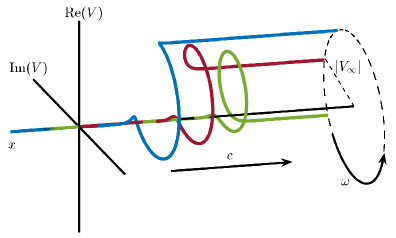
for some , . In Figure 1.1 we illustrate the profile of such a wave and its motion in an frame. The wave belongs to the class of front-type modulated waves as classified by Sandstede and Scheel in [22, Sec. 2.2]. However, it does not asymptote to wave trains in both directions , hence, in a strict sense, does not fall into their category of defects; see [7, Introduction] for a more detailed comparison. Note that we used the term traveling oscillating front (TOF) in [7] to denote this specific type of wave. Waves of the form (1.3) with (1.4) occur in the so called bistable regime, i.e. they connect the stable equilibrium at with the spatially homogeneous state at which belongs to a stable limit cycle of the ODE obtained from (1.1) as . Numerical simulations of such waves are shown in [7, Introduction], and we note that there is numerical and theoretical evidence for their generic occurrence in QCGL (cf. [24]).
The goal of this work is to prove asymptotic stability with asymptotic phase of the solutions to the perturbed problem
Our main result Theorem 2.1 assumes the initial perturbation and its derivative to decay algebraically sufficiently fast, i.e.
| (1.5) |
Then we conclude algebraic decay both in space and time for the perturbed solution as follows:
| (1.6) |
where , . The value is the asymptotic phase which is approached by one order less in time than the shifted profile. In fact, the asymptotics above hold in suitable weighted Sobolev spaces as specified in (2.8), (2.9). The result complements our main theorem from [7] where was allowed to be the sum of an exponentially localized function and of a profile which limits at to a small but nonzero value.
The coupling of algebraic decay rates in space for initial perturbations to algebraic decay rates in time is a well-known phenomenon in stability studies of nonlinear waves. As a general rule, it occurs when the essential spectrum of the linearization touches the imaginary axis at the origin. In the following we discuss some results of this type in the literature and expand on differences and similarities to our work.
One of the most studied topics is the so-called marginal stability of critical fronts in the Ginzburg-Landau equation; see the work of Avery and Scheel [2, 3, 4] and the early contribution [9]. The recent works [3, 4] give a rather comprehensive overview of the development of the theory. Critical fronts typically occur in the cubic Ginzburg-Landau equation and belong to the monostable case. There are several differences when compared to the bistable case above: in addition to translation and gauge invariance which is also present in our case, there is a whole interval of velocities of which only the extreme one is marginally stable; as a result one has to require exponential decay of the invading perturbation which is not needed in our result above. The proofs have several similarities, such as the algebraically weighted resolvent estimates via suitable contours, but differ in technical details, such as the additive decomposition used in (1.6) when compared to the polar coordinate ansatz used in [4]. We also mention that the time rates for the critical fronts in [4] are shown to be optimal while the threshold in (1.5), (1.6) is open for improvement. However, we expect, as a general phenomenon, that the spatial rate for the initial data in (1.5) splits into a spatial rate and a temporal rate for the perturbed solution in (1.6).
Next we mention the work of Kapitula [17, 15] who derives a stability result w.r.t. the -norm for a version of (1.1) with a specific form of the nonlinearity and a small imaginary part of the diffusion coefficient ; see [15, Theorem 7.2]. The analysis proceeds via the associated Evans function and algebraic time estimates are restricted to a particular parameter set ( in [15, Theorem 7.2]), while exponential weights are required for the general case. Moreover, the decomposition of the dynamics is slightly different from ours and some technical arguments of the algebraic estimates need to be corrected; see Lemma 3.5 and Remark 3.6 for more details.
In the following we give a rough outline of the subsequent sections and emphasize the major mathematical arguments. In Section 2 we list the assumptions and formulate our main result Theorem 2.1 in algebraically weighted Sobolev spaces. In Section 3 we analyze in detail the spectrum of the operator obtained by linearizing about the wave (1.3) in a co-moving frame. Our assumptions lead to quadratic contact of the essential spectrum with the imaginary axis (Figure 3.1) and we use the theory of exponential trichotomies (Appendix A) to handle the separation of spatial modes on the positive axis into a weakly and a strongly exponentially decaying part. This serves as a suitable preparation for the resolvent estimates (Proposition 3.7) which hold in a crescent-like domain of the complex plane (Figure 3.1). In the ensuing sections we derive algebraic decay rates for the semigroup generated by the linearized operator (Theorem 4.1) and decompose the nonlinear dynamics into an equation along the shifted profile and orthogonal to it (Lemma 5.1, Eq.(6.1)). Using remainder estimates in algebraically weighted Sobolev norms (Lemma 5.2) and a Gronwall lemma adapted to algebraic integral kernels (Lemma 6.2) allows us to conclude nonlinear stability (Theorem 6.3).
2 Assumptions and main results
Instead of working with the complex-valued equation (1.1) it is convenient to analyze the corresponding real-valued system as a classical reaction diffusion equation. With , , , and , we rewrite (1.1) equivalently as
| (2.1) |
where
| (2.2) |
A front-type modulated wave of (2.1) is then given by a particular solution of the form
where and the profile satisfies
| (2.3) |
Here the asymptotic rest state is given by . Next, it is natural to transform (2.1) into a co-moving frame by setting , so that solves (2.1) if and only if solves
| (2.4) |
Then the profile becomes a stationary solution of (2.4), i.e.,
| (2.5) |
To obtain the stability of the stationary solution of (2.4), we study the long time dynamics of the perturbed initial value problem
| (2.6) |
where the initial perturbation is small in a suitable sense. The stability behavior or long time dynamics of the solution of (2.6) strongly depends on the norm in which is measured. Before making this precise, let us collect our basic assumptions for the system (2.6).
Assumption 1.
The coefficient and the function satisfy
Assumption 2.
There exists a front-type modulated wave solution of (2.1) with profile , speed , frequency , and asymptotic rest state such that
Recall that one can multiply the wave by a phase factor so that the rest state has this particular form.
Assumption 3.
The coefficient and the function satisfy
The linearization of (2.6) at the profile is given by the operator
| (2.7) |
In general, we consider as a linear operator on a Banach space defined on a domain and write if is a closed and densely defined linear operator. A simple example is so that with . In any case, for we denote its resolvent set by
and its spectrum by . The spectrum is subdivided into the point spectrum
and the essential spectrum . Let us denote by the nullspace of .
Assumption 4.
For the operator from (2.7) with there is such that holds for all . Moreover,
Indeed, we show that is spanned by . However, it turns out that is not Fredholm of index so that and does not belong to an eigenvalue in .
In order to specify the smallness of the perturbation in (2.6), we introduce the algebraic weight function of linear growth
Further, let us define associated algebraically weighted Lebesgue spaces for arbitrary :
| (2.8) |
and Sobolev spaces for
| (2.9) | ||||
With theses preparations we state our main result.
Theorem 2.1.
Let Assumption 1-4 be satisfied and let be given with . Then there exist constants , such that the following statements hold for all initial perturbations which satisfy : The initial-value problem (2.6) has a unique global solution which can be represented as
for suitable and . Further, there is an asymptotic phase with such that the following estimates hold for :
| (2.10) |
where for , .
In Remark 6.4 we explain in detail how the value of the exponent arises from the interaction of linear and nonlinear terms.
3 Spectral analysis of the linearized operator and resolvent estimates
In this section we discuss the spectral properties of the linearized operator from (2.7) considered as an operator on the algebraically weighted space for some . We will derive sharp estimates of the solution to the resolvent equation
| (3.1) |
where with suitable and where lies in various subdomains of .
3.1 Resolvent estimates for large -values and the dispersion set
We begin with collecting basic properties of proved by standard estimates.
Lemma 3.1.
Proof.
As a next step we characterize the essential spectrum of . In [7] the essential spectrum of was determined for in exponentially weighted -spaces. In general, there is a well developed spectral theory for second order differential operators on the real line in the context of traveling waves; we quote [16] and [21] as general references. It is well known that the Fredholm properties of and therefore its essential spectrum is invariant under algebraic weights of the underlying -space. In particular, the essential spectrum of coincides with the essential spectrum of . This is a consequence of the invariance of the Fredholm index under compact perturbation [12, Chapter IX] and can be shown along the lines of [7, Lemma 3.2]. Another compact perturbation argument shows that the operator is Fredholm for in the set
| (3.3) | ||||
with Fredholm index . The matrices refer to the limits at of the matrix in the corresponding first order system; see (3.4) below. Hyperbolicity means that there are no eigenvalues on the imaginary axis and denote the dimension of the stable subspaces of for (see e.g. [16, Lemma 3.1.10]). Analyzing the eigenvalue problem for then yields with the dispersion set
With these results in mind, the following theorem is a consequence of [7, Theorem 3.5].
Theorem 3.2.
Proof.
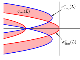
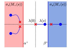
In Figure 3.1 we show the essential spectrum and the dispersion set for the QCGL with parameters and , , in (1.2). In general, the dispersion set consists of four curves in which lie in the complement of the rounded sector pointed at zero. One of the curves in is critical; it touches the imaginary axis at the origin in a quadratic fashion so that . As we will see later, this is due to the fact that one of the (spatial) eigenvalues of (denoted by later in this section) crosses the imaginary axis when crosses the critical curve from right to left. Thus, the appearance of eigenfunctions in the non-empty kernel as well as the essential spectrum touching the imaginary axis prevent uniform bounds of the resolvent to hold for near the origin and for functions in which solve (3.1) with . But, as we will show, restricting the class of right hand sides to a codimension subspace of for some allows for such uniform bounds and sharp resolvent estimates close to the origin, but to the right of the dispersion set.
3.2 Spectral analysis via dichotomies and trichotomies
In this subsection we characterize dichotomies and trichotomies of the first order system for equivalent to (3.1) and given by
| (3.4) | ||||
By we denote the solution operator of (3.4) which is analytic in , i.e., the function , solves the initial value problem , for , . The notion of dichotomies and trichotomies that we use throughout the paper is recalled in Appendix A. These properties will be crucial for the resolvent estimates in the subsequent sections.
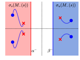
The first step is to analyze the eigenvalues of the limiting matrices from (3.3). In particular, when moves from to some , the eigenvalues of move as sketched in Figure 3.2: has two stable and two unstable eigenvalues which do not cross the imaginary axis while has two stable eigenvalues, an unstable one that stays real positive, and then a critical real one which moves from zero to the right. Since we allow multiple eigenvalues for the groups of two it is convenient to work with invariant subspaces and spectral subsets rather than eigenvectors and eigenvalues (a viewpoint stressed in the monograph [23] when compared to the classical reference [18, Ch.2]). The following lemma deals with a specific perturbative situation which needs a separate proof.
Lemma 3.3.
Let Assumption 1-3 be satisfied. Then there exist and such that the following statements hold for :
-
(i)
The matrix is hyperbolic with stable subspace of dimension and unstable subspace of dimension . The corresponding spectral projectors , of rank are analytic in and satisfy
(3.5) -
(ii)
The spectrum of can be decomposed into three subsets with associated spectral projectors , , which are of rank , , respectively, and which depend analytically on . They satisfy the estimates
(3.6) The central projector is of the form where , and holds. Further, satisfies
(3.7) The eigenvalue is simple and analytic in , and it has the properties
-
(a)
for ,
-
(b)
, , ,
-
(c)
if .
-
(a)
Proof.
Lemma B.1(i) applies to since and have a positive lower spectral bound due to Assumption 1. Hence is hyperbolic with two-dimensional stable and unstable subspace and corresponding projectors , . Then there is a norm in such that
This property persists for small with Riesz projectors analytic in and given by
| (3.8) |
where are semicircles with sufficiently large radius enclosing the stable and unstable subsets and parameterized by
In particular, there exist and such that we have for
| (3.9) |
Taking powers for with this norm and filling the gaps by continuity then leads to the estimate (3.5) using the equivalence of norms and .
The proof of (ii) is somewhat more involved. By Assumption 2 we have so that has a simple eigenvalue with eigenvector and another simple eigenvalue . Using further , Lemma B.1(ii) ensures that has a two-dimensional stable subspace, a one-dimensional unstable subspace and a one-dimensional critical subspace which belongs to the zero eigenvalue. The critical right eigenvector and left eigenvector of are given by
| (3.10) |
The spectral projectors of rank and of rank can be continued analytically for as in (3.8). Similarly, the rank projector is continued analytically by
if and are chosen such that the curves and do not overlap. For the stable and the unstable projection we obtain contraction as in (3.9) and then the exponential estimates (3.6). Another method of determining the unique central projector is via the analytic implicit function theorem applied to the mapping
| (3.11) |
for which holds. The derivative w.r.t.
is invertible since is a simple eigenvalue of . The local solution , of satisfies and solves the eigenvalue problem
| (3.12) |
From a suitable adjoint system we obtain analytic left eigenvectors normalized by . Setting , where , then leads to the representation with . The estimate (3.7) follows directly from this representation.
Assertion (a) follows since the real implicit function theorem equally applies to from (3.11) when restricted to . By uniqueness we then have for as well as . We differentiate (3.12) at and find using (3.10)
| (3.13) |
Multiplying by yields , hence . Moreover, solving (3.13) for and using Assumption 3 yields where
Differentiating (3.12) twice at and multiplication by leads to
hence . Finally, we establish (c) by using the Taylor expansion
| (3.14) |
Since we have for and some . This implies for real . Otherwise and we can write where . In the following we consider where is still to be determined. We insert into (3.14) and obtain
If we find for sufficiently small
Since there exists a constant such that
In case we obtain for small and suitable
Finally, this leads to
which finishes the proof. ∎
Using the roughness theorems [10, Proposition 4.1] and Theorem A.1 we establish analogous estimates for the variable coefficient operator from (3.4).
Lemma 3.4.
Let Assumptions 1-3 be satisfied, let , , be given by Lemma 3.3, and take any with . Then the following statements hold for and sufficiently small:
-
(i)
The operator has an exponential dichotomy on with data
where for each the projectors depend analytically on and have rank . -
(ii)
The operator has an exponential trichotomy on with data
where is given by Lemma 3.3 (ii) and the projectors have rank and . The exponents satisfy and the following estimates hold:(3.15)
Proof.
By [7, Theorem 2.5] there are such that we have for
Then the first assertion is a consequence of Lemma 3.3 and [10, Proposition 4.1]. For the second assertion recall the ordinary exponential trichotomy of on . Let be the left and right eigenvectors of associated with the eigenvalue from Lemma 3.3. Then solves and solves the adjoint system on . Further, the central projector is given by and the functions and are constant w.r.t. . By [7, Theorem 2.5] there exist such that for all
Applying Theorem A.1 we conclude that has an ordinary exponential trichotomy on and we can choose the exponents , arbitrarily close to such that the estimates (3.15) hold. ∎
3.3 Resolvent estimates for the linearized operator
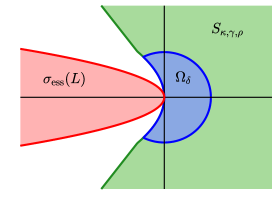
In this subsection we study the resolvent equation (3.1) of the linearized operator for right hand sides with suitable and for in a suitable neighborhood of the origin. This neighborhood has the shape of a crescent (see Figure 3.1) with a parabolic section determined by the value of from the rounded sector in Theorem 3.2 and by from Lemma 3.3(ii)(c). We assume w.l.o.g. and define the -crescent by
| (3.16) |
In the following we take sufficiently small and we recall that by the definition of . We aim to show uniform bounds of the resolvent for w.r.t. suitable norms. Since the essential spectrum of touches the imaginary axis quadratically at the origin (Theorem 3.2) a singularity of the resolvent of occurs at . In particular, this prevents us from showing uniform bounds for the resolvent on for . Instead, we assume a stronger decay of the right hand side in (3.1), i.e., for some , and show uniform bounds in of the resolvent as an operator from to . In addition, we resolve the order of the singularity caused by the essential spectrum in dependence on when . The approach uses the exponential dichotomy and exponential trichotomy of the first order operator from Lemma 3.4 and the following estimates.
Lemma 3.5.
The following statements hold:
-
1.
For every and with either or there exists such that for all and :
(3.17) The estimate (3.17) still holds in case and .
-
2.
For every there is such that for all and
(3.18) -
3.
For every and there exists such that for all and :
(3.19)
Remark 3.6.
Lemma 3.5 is an extension and a correction of [17, Lemma 3.2], [15, Lemma 3.3]. The extension concerns and to be noninteger in (3.17), (3.19), the new estimate (3.18), and the use of the weight function which avoids a case-by-case analysis of and . The correction concerns the estimate (3.19) which is claimed there to hold with for all . For our estimate is an improvement, while for it corrects a flaw in [17, Lemma 3.2]. Let us further note that the forthcoming estimates will use counterparts of (3.17) and (3.19) on which are obtained by reflection.
Apart from the singularity of the resolvent caused by the essential spectrum, another difficulty appears since has a nontrivial kernel caused by the translation invariance of (2.1). Roughly speaking, there is an "eigenvalue" hidden in the essential spectrum at the origin. The strategy then is to
split the space , into and into its orthogonal complement. In this way
we obtain uniform resolvent estimates on the complement while simultaneously keeping track of the singular growth of the resolvent on .
Proposition 3.7.
Let Assumption 1-4 be satisfied and let . Then there exists and for every , a constant such that the system (3.4) has a unique solution for all and . This solution satisfies the estimates
| (3.20) | |||||
| (3.21) |
where the map is given by
and is the unique bounded solution of the adjoint system
| (3.22) |
If with then , can be continuously extended by some which solves (3.4) for and which satisfies .
Remark 3.8.
Writing is a slight abuse of notation since is only bounded. However, the integral of exists for and holds; see (3.34).
Proof.
Step 1: Dichotomies and Trichotomies
In the following we frequently use the dichotomy resp. trichotomy of on resp. provided by
Lemma 3.4. Let us further note that the -derivatives of solutions inherit the exponential estimates by Cauchy’s theorem, i.e., for and sufficiently small , we have for
| (3.23) |
and for
| (3.24) |
Analogous estimates hold for the complementary projectors. In the following we prove the assertion for . Let be matrices such that , and define for
By Lemma 3.4 the matrix functions
| (3.25) |
solve the homogenous equation (3.4) and satisfy the exponential estimates
Further, by Assumption 4 we have , hence there exist with
There also exists some with , . The solution operator of the adjoint is given by
It has an exponential dichotomy with data
and, likewise, it has an exponential trichotomy with data
| (3.26) |
Step 2: The simple eigenvalue
From we have
where we abbreviate . In view of (3.26) the space of bounded solutions of the system (3.22) is one-dimensional and spanned by . Further, satisfies the estimate
| (3.27) |
In the following we show that is a simple eigenvalue of , i.e. and . Assuming the contrary, there exist such that
With these data the function defined by
is continuous at . Moreover, it satisfies the inhomogenous variational equation obtained by differentiating for w.r.t. at :
| (3.28) |
Rewriting this for the first part of shows and . Finally, the exponential estimates (3.23) and (3.24) imply exponential decay of the -derivatives and then of and its first derivative due to (3.28). Thus we find that is a generalized eigenfunction of that belongs to the eigenvalue . This contradicts Assumption 4.
Now we can normalize such that holds. Then Keldysh’s Theorem (see e.g. [6, Theorem 2.4]) gives a representation of the inverse near . There exists and an analytic function such that
| (3.29) |
Using (3.28) and integration by parts the normalization is rewritten as follows:
Step 3: Construction of the solution
Let us define for two Green’s functions via
So far, we have worked with , but from now on we restrict to . First consider particular solutions of the inhomogeneous equation (3.4) on
| (3.30) | ||||
where are given by (3.25) and are determined to ensure continuity of at , i.e.
With (3.29) we write the solution for as
| (3.31) |
For the principal term we use and the definition of :
Inserting this into (3.30) and using leads to the following expression for
| (3.32) | ||||
In a similar way we obtain for
| (3.33) | ||||
Step 4: Estimates for
We show (3.20) and (3.21) for on by estimating term by term in
(3.32). The estimates of on via the terms in (3.33) are
somewhat simpler (because of the dichotomies) and are therefore omitted here.
For the first term in (3.32) we note that holds for all due to the
exponential decay and due to (3.27). This leads to
| (3.34) |
For the second term we have from (3.23) that holds for and yields
For the third term in (3.32) we first estimate as follows:
where we used that and are uniformly bounded for and ; see (3.23), (3.24). This gives for the third term in (3.32) the estimate
| (3.35) |
The fourth term in (3.32) involves the stable projector . We use (3.19), the Cauchy-Schwarz inequality, and Fubini’s theorem, to obtain
Next we estimate the last term in (3.32) which is the critical term since it involves the central projector through . We decompose it into
Since for all we obtain by using (3.17) with and instead of , Cauchy-Schwarz inequality, and Fubini’s theorem
| (3.36) | ||||
If we can replace by in (3.36) and obtain
| (3.37) | ||||
It is here that we need the stronger norm . Collecting the estimates above we infer (3.21) for on in case . If we have only with then we modify the estimate of the critical term from (3.37) by using (3.17), (3.18), and (3.15):
where the last inequality uses the estimate from Lemma 3.3 (ii) b), c) for . Together with the estimates above this proves (3.20) for on in case . Combining this with the corresponding estimates on proves our assertions (3.20) and (3.21) for .
Step 5: The case
Let us reconsider steps 3 & 4 in case with and let . Then we have and
(3.31) shows that
is continuous at . Moreover, the term drops out from the definition of in
(3.32), (3.33) and the subsequent estimates (3.35)-(3.37) still hold for and . Continuity of the integral expressions (3.32), (3.33) at
follows from the uniform bounds (3.21) and the pointwise convergence of the integrands via Lebesgue’s theorem.
∎
As a consequence of Proposition 3.7 we obtain an estimate for the solution of the resolvent equation (3.1) in a sufficiently small -crescent .
Corollary 3.9.
Let Assumption 1-4 be satisfied and let . Then there exist and for every , a constant such that the equation has a unique solution for all and . This solution satisfies the estimates
| (3.38) | |||||
| (3.39) |
Here is the projector given by
and is the unique bounded solution of the adjoint system
| (3.40) |
If with then , can be continuously extended by some which solves and which satisfies the estimate .
Proof.
By a straightforward calculation we find that the equation
holds if and only if . Setting and taking (3.4) into account yields
where appears in the first component. By (3.22) the normalization is
Hence, Proposition 3.7 shows that (3.40) has a unique bounded solution. Further, the setting transfers the estimate (3.21) to our assertion (3.39). This one uses the estimate of the projector which is analogus to (3.34):
This completes the proof. ∎
Corollary 3.9 suggests to introduce the following subspaces for
This leads to the decompositions and . Further, holds since for we have and
Remark 3.10.
In fact, one can show that the operator with domain is a closed operator from to and Fredholm of index ; cf. [11, Sec. 5.3]. Taking the subspaces into account then implies that the operator is invertible.
4 Semigroup estimates
In this section we use the estimates from Corollary 3.9 to construct and prove algebraic decay of the semigroup generated by . From Lemma 3.1 and Theorem 3.2 we conclude that the operator from (2.7) lies in , is a sectorial operator, and generates an analytic semigroup denoted by . Moreover, Assumption 4 guarantees the spectral bound at zero, hence there exists such that for the following estimates hold
| (4.1) |
Note that (4.1) is not sharp for large in the sense that in fact we have the bounds and for arbitrary . However, for simplicity we chose so that is fixed.
The essential spectrum of touching the imaginary axis at the origin prevents the semigroup to have exponential decay.
Instead, we use the sharp resolvent estimates of the previous sections to show algebraic decay of the semigroup for
initial data from a proper subspace.
Theorem 4.1.
Proof.
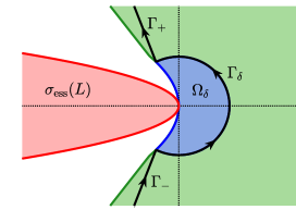
We first prove (4.2) for the case : Define oriented contours running upwards and running counterclockwise in the complex plane (see Figure 4.1 (left)).
where and with from Lemma 3.1. If we choose sufficiently small we have
By further taking and sufficiently small, we can ensure, by Assumption 4 and Theorem 3.2, that the concatenated contour satisfies for and that there is no spectrum of to the right of in the complex plane.
Using the sectorial estimates from Lemma 3.1, standard semigroup theory (see e.g. [14, 20, 19]) implies that
defines an analytic semigroup on satisfying (4.1) for any and all , . The boundary of the closure is given by the contour with the parabolic curve (see Figure 4.1 (right))
If holds, then by Corollary 3.9 the function , has a continuous extension to which we write as . In this sense the integral
| (4.3) |
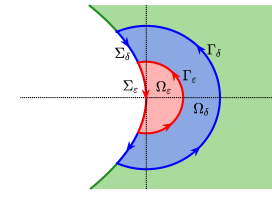
exists in . We show that it vanishes although is not contained in an open domain of analyticity of the resolvent 111Note that is not a removable singularity in the classical sense which requires analyticity to hold in a pointed neighborhood.. For that purpose, let be the -crescent according to (3.16) for . Since the resolvent is analytic in an application of Cauchy’s integral theorem and of the uniform estimates from Corollary 3.9 imply
| (4.4) |
as . Using Corollary 3.9 and (4.4) this gives for and for a generic constant
Further, for we have due to
| (4.5) | ||||
Using the exponential bounds (4.1) for we conclude for ,
| (4.6) |
If is an arbitrary integer, i.e. , we can apply (4.6) -times to obtain
Replacing by yields the first estimate in (4.2) for . The second one follows analogously from the second estimate in (4.6).
Let us now consider the case for arbitrary and assume . We decompose with and . If , the estimate (4.2) immediately follows by our previous observations and the inclusion . So let . Using the resolvent estimate (3.38) from Corollary 3.9 we observe that the integral (4.3) exists even in since we can estimate:
Further, the estimate (3.38) from Corollary 3.9 now yields for and a generic constant
With (4.5) and the exponential bounds (4.1) this yields for and
We obtain the first estimate in (4.2) as follows:
As before, the second estimate in (4.2) for the general case follows by similar arguments. This completes the proof. ∎
5 Decomposition of the dynamics and nonlinearities
We decompose the solution of the perturbed co-moving system (2.6) into
| (5.1) |
so that describes a motion along the group orbit and describes a perturbation perpendicular to the nullspace of the adjoint operator spanned by from Corollary 3.9. We follow the lines of [7, 8] to show that the decomposition (5.1) is unique as long as the solution stays close to the profile and further derive a system of evolution equations that determines the dynamics of and . We define the maps
| (5.2) |
and
| (5.3) |
Lemma 5.1.
Proof.
First note that for every the function is continuous in and decays exponentially at due to Assumptions 1, 2 and [7, Thm. 2.5]. Therefore, is well-defined and continuously differentiable due to Corollary 3.9 and satisfies and . Thus the assertion for is a consequence of the inverse function theorem. Similarly, is continuously differentiable and satisfies with which is invertible due to the decomposition . Hence, by the inverse function theorem, is a local diffeomorphism and one concludes the identity (5.4) by applying to the equation . ∎
Assuming that (2.6) has a solution , for some such that for all , i.e., the solution stays in the region where exists, we find unique and such that
and the decomposition (5.1) holds for all . In this case, we have and we can set the initial values for and as
| (5.5) |
If for we insert (5.1) into (2.6) and obtain
where we used for all by the equivariance of the stationary co-moving equation (2.5). This leads to
| (5.6) |
with the nonlinear remainder
Recall the projector from Corollary 3.9 and define the continuous linear map
Since we can assume w.l.o.g. that for all so that the inverse of , exists and is given by
| (5.7) |
Note that is continuously differentiable w.r.t. . Applying first and then to (5.6) and using , we obtain a system of evolution equations for and
| (5.8) | |||||
| (5.9) |
with from (5.5) and the nonlinear remainders
| (5.10) | ||||
| (5.11) |
Next we derive Lipschitz estimates for the nonlinearities in (5.10), (5.11).
Lemma 5.2.
Proof.
We denote by a generic constant and choose so small such that and with from Lemma 5.1 so that the remainders are well-defined. The main idea for handling the different algebraic rates is to use the following estimates for all that are simple consequences of standard Sobolev embeddings ():
| (5.17) |
and due to Assumption 1, 2 and [7, Thm. 2.5]
| (5.18) | ||||
In fact, the remainders are quadratic so that we can frequently make use of the estimates (5.17), (5.18) in the following. We abbreviate and obtain, since is smooth due to Assumption 1,
The estimate for the derivative follows by similar arguments and by using so that (5.12) holds. For (5.13) we estimate, using the exponential convergence of at from [7, Thm. 2.5],
Again the estimate of the derivative follows analogously and one infers (5.13). The estimates (5.14), (5.15), (5.16) follow from (5.12) and (5.13) and using the boundedness of from Corollary 3.9 and the smoothness of from (5.7); see [11] for more details of the estimates. ∎
6 Nonlinear stability
In this section we prove our main result, Theorem 2.1. Assuming suffciently small initial perturbation w.r.t. sufficiently high algebraic rates we prove stability of the solution of the decomposed system (5.8), (5.9) which then lead to the stability of the original system (2.6). More precisely, we work the corresponding integral equations of (5.8), (5.9), reading as follows:
| (6.1) | ||||
Using the semigroup estimates from Theorem 4.1 and the Lipschitz estimates from Lemma 5.2 we show global existence of a solution and algebraic decay of the perturbation in (6.1) by applying a Gronwall argument. The transformation (5.1) then leads to the stability of the original system (2.6).
As a first step we establish the existence of a local (mild) solution of (6.1) by a standard contraction argument using the exponential estimates of the semigroup from (4.1). Since the proof is rather standard and fully analogous to the proof of [7, Lemma 7.1], it is omitted here.
Lemma 6.1.
Next we extend the local solution from Lemma 6.1 to a global solution such that the perturbation decays algebraically. For this we use the following Gronwall estimate involving algebraic integral kernels.
Lemma 6.2.
Suppose , and such that
and let for some satisfying
Then for all there holds
Proof.
We estimate for
where we used the bound for all . Now let
and note that follows from . Now assume . Then and our assumptions imply
This is a contradiction, so that follows, and our assertion is proved. ∎
Now we are in the position to prove the analogue of our main result for the -system (6.1).
Theorem 6.3.
Proof.
Recall the constants from (4.1), from (4.2) and from Lemma 5.2. Choose such that
| (6.6) |
We abbreviate and let
Then Lemma 6.1 with and implies . Using Theorem 4.1 and Lemma 5.2 (with and ) we estimate for all
Thus the Gronwall estimate in Lemma 6.2 (with ) implies due to (6.6)
| (6.7) |
This yields, due to and (6.6), for all
| (6.8) | ||||
Next we show . Assuming the contrary, , then the estimates (6.7), (6.8) imply
Setting and we can apply Lemma 6.1 to the system (6.1) with initial values and obtain a solution on such that and for all . Then the concatenated functions
define a solution of (6.1) on with and for all . This contradicts the definition of , so that follows. The estimate (6.3) is a consequence of (6.7). For (6.4) we estimate with Lemma 5.2 and (6.7) the integral
| (6.9) | ||||
Thus, the asymptotic phase
exists and (6.4) holds due to (6.9). The estimate (6.5) is a simple consequence of (6.4). Next we show the regularity of the solution . From Lemma 5.2 one infers , so that . Now let for . Then is Lipschitz continuous since with Lemma 5.2 we have for all
for some . In particular, is Hölder continuous with index , i.e., , and for arbitrary
The standard theory of parabolic equations, e.g. [1, Theorem 1.2.1] and [14, Theorem 3.2.2], now implies that is the unique solution of (5.8), (5.9) in the class (6.2) and that holds for every . This completes the proof. ∎
Remark 6.4.
Let us recall the restriction on the values of and that determines the required algebraic decay of the initial perturbation in Theorem 6.3. Roughly speaking, Theorem 4.2 guarantees an algebraic decay of the semigroup for arbitrary . Then the Gronwall Lemma 6.2 gives an algebraic decay of in of one degree less, i.e., . This is caused by the semigroup which involves an integration in time and hence costs another degree. The convergence of the shift to the asymptotic phase needs an additional integration in time, so that . This requires and therefore . To ensure the assumptions for the Gronwall argument in the proof of Theorem 6.3 we need which leads to . Summarizing, the weakest possible condition on the initial data is to make small so that Theorem 6.3 applies with and sufficiently small.
Proof of Theorem 2.1.
Let be such that by Lemma 5.1 the map (resp. ) exists and is diffeomorphic on (resp. on ), i.e., we may choose so small such that (resp. ). Let
and let such that for all . Next we choose such that every solution of (5.8), (5.9) from Theorem 6.3 satisfies and for all . We restrict the size of the initial perturbation to
Set so that we have
This implies so that the solution of (5.8), (5.9) with initial value from Theorem 6.3 and the asymptotic phase satisfy (2.10). Then the function
belongs to and satisfy (2.6) by the computation in Section 5. It remains to show the uniqueness of . We note that for all we have by Theorem 6.3
Let be another solution of (2.6) on for some and let
Then there are solving (5.8), (5.9) on with initial value and such that for all . But then and on by the uniqueness of . Assuming , we have for
Thus and on . This finishes the proof. ∎
Acknowledgements
This paper is an extended version of parts of the second author’s PhD Thesis [11]. His present work was funded by the Deutsche Forschungsgemeinschaft (DFG, German Research Foundation) under Germany’s Excellence Strategy – EXC-2047/1 – 390685813. The work of the first author was funded by the Deutsche Forschungsgemeinschaft (DFG, German Research Foundation) – SFB 1283/2 2021 – 317210226.
References
- [1] H. Amann. Linear and quasilinear parabolic problems. Monographs in mathematics. Birkhäuser, Basel, 1995.
- [2] M. Avery and A. Scheel. Asymptotic stability of critical pulled fronts via resolvent expansions near the essential spectrum. SIAM J. Math. Anal., 53(2):2206–2242, 2021.
- [3] M. Avery and A. Scheel. Universal selection of pulled fronts. Comm. Amer. Math. Soc., 2:172–231, 2022.
- [4] M. Avery and A. Scheel. Sharp decay rates for localized perturbations to the critical front in the Ginzburg–Landau equation. J. Dynam. Differential Equations, 36:287–322, 2024.
- [5] W.-J. Beyn. On well-posed problems for connecting orbits in dynamical systems chaotic numerics. Contemporary Mathematics, 172, 131, 1994.
- [6] W.-J. Beyn. An integral method for solving nonlinear eigenvalue problems. Linear Algebra and its Applications, 436, 10, 3839, 2012.
- [7] W.-J. Beyn and C. Döding. Stability of traveling oscillating fronts in complex Ginzburg Landau equations. SIAM J. Math. Anal., 54(5):5447–5488, 2022.
- [8] W.-J. Beyn and J. Lorenz. Nonlinear stability of rotating patterns. Dynamics of Partial Differential Equations, 5(4):349–400, 2008.
- [9] J. Bricmont and A. Kupiainen. Stability of moving fronts in the Ginzburg-Landau equation. Comm. Math. Phys., 159(2):287–318, 1994.
- [10] W. A. Coppel. Dichotomies in stability theory, volume 629 of Lecture notes in mathematics Series: Australian National University, Canberra. Springer, Berlin, 1978.
- [11] C. Döding. Stability of traveling oscillating fronts in parabolic evolution equations. PhD thesis, Department of Mathematics, Bielefeld University, 2019.
- [12] D. E. Edmunds and W. D. Evans. Spectral theory and differential operators. Oxford mathematical monographs. Oxford University Press, Oxford, 2nd edition, 2018.
- [13] J. K. Hale and X.-B. Lin. Heteroclinic orbits for retarded functional-differential equations. Journal of Differential Equations, 65, 2, 175, 1986.
- [14] D. Henry. Geometric theory of semilinear parabolic equations, volume 840 of Lecture notes in mathematics. Springer, Berlin, 1981.
- [15] T. Kapitula. On the stability of travelling waves in weighted spaces. Journal of Differential Equations, 112(1):179–215, 1994.
- [16] T. Kapitula and K. Promislow. Spectral and dynamical stability of nonlinear waves, volume 185 of Applied mathematical sciences. Springer, New York, 2013.
- [17] T. M. Kapitula. Stability of weak shocks in – systems. Indiana University Mathematics Journal, 40, 4, 1193, 1991.
- [18] T. Kato. Perturbation theory for linear operators, volume 132. Springer, Berlin, 1966.
- [19] A. Pazy. Semi-groups of linear operators and applications to partial differential equations, volume 10 of Lecture notes, University of Maryland, Department of Mathematics. College Park, Md., 1974.
- [20] M. Renardy and R. C. Rogers. An introduction to partial differential equations, volume 13 of Texts in applied mathematics. Springer, New York, 2nd edition, 2009.
- [21] B. Sandstede. Stability of travelling waves. In B. Fiedler, editor, Handbook of Dynamical Systems, volume 2, pages 983–1055. Elsevier, 2002.
- [22] B. Sandstede and A. Scheel. Defects in oscillatory media: Toward a classification. SIAM Journal on Applied Dynamical Systems, 3(1):1–68, 2004.
- [23] G. W. Stewart and J. G. Sun. Matrix perturbation theory. Academic Press Inc., Boston, 1990.
- [24] W. van Saarloos and P. Hohenberg. Fronts, pulses, sources and sinks in generalized complex Ginzburg-Landau equations. Physica D, 56(4):303–367, 1992.
Appendix A Roughness of exponential trichotomies
Considering a linear differential operator on an interval and with . Let be the solution operator of , i.e., solves in with . Then the operator is said to have an ordinary exponential trichotomy on with exponents if is there is a constant and projectors , of rank such that and such that for all there hold
In the case we call the data of the ordinary exponential trichotomy. If we speak of a shifted exponential dichotomy and if, in addition, we speak of an exponential dichotomy. There are several results regarding the preservation of an exponential trichotomy (or dichotomy) under suitable perturbations of the matrix-valued function ; see e.g. [10], [13], [5]. We prove a new so called Roughness Theorem for ordinary exponential trichotomies.
Theorem A.1 (Roughness theorem).
Let be a bounded domain, and let , , , have an ordinary exponential trichotomy on for every with data , depending continuously/analytically on . Further assume that is of rank and has the form where on and such that there are with
Let with , for some . Then the perturbed operator has an ordinary exponential trichotomy on with data depending continuous/analytically on and with independent of . In particular, and are given by and where
Proof.
We denote by a generic constant independent on and . It is sufficient to prove the assertion for the interval instead of where is so large that the following condition is satisfied:
| (1.1) |
Consider the shifted operator which has an ordinary exponential trichotomy on with data . Setting , and , we obtain that has a shifted exponential dichotomy on with data and a shifted exponential dichotomy on with data . With the roughness theorem for exponential dichotomies [10, Chap. 4, Prop. 1] implies due to (1.1) that the perturbed operator has a shifted exponential dichotomy on with data
and a shifted exponential dichotomy on with data
Furthermore, it is shown in [5, Prop. 2.4] that the projectors satisfy the estimates
| (1.2) |
In addition, the ranks of the projectors are preserved, i.e., , , for all . This implies, due to , that with codimension equal to so that there is with . Next, we show that can be chosen such that satisfies
| (1.3) |
where and where is the solution operator of .
Consider for the map
| (1.4) | ||||
Due to the assumptions we have so that we have the estimate
| (1.5) | ||||
with independent on . Similarly, we have for the estimate . Since , due to (1.1), is a contraction on so that there exists such that for all . Further, depends continuously/analytically on , since does. Using the definition of from (1.4) one shows that solves on and as in (1.5)
where we used the a-priori bound . Now we have since
since . Assuming we obtain
where we used . This is a contradiction and therefore . This shows, after normalization of , that on and (1.3) holds. Now take such that
Setting , where is the solution operator of the adjoint , we find that is the projector onto satisfying . Moreover, depends continuously/analytically on , since does, and from (1.2) we deduce the estimate for . By assumption and the estimate (1.3) we have that is uniformly bounded from below. This gives
Finally this implies for all
With and we have shown that the operator has an exponential trichotomy on with data
depending continuously/analytically on and some independent on . Now the assertion for follows. ∎
Appendix B A matrix lemma
For a matrix define its lower spectral bound by and note that if .
Lemma B.1.
Let and . Then the block matrix
has the following properties:
-
(i)
If and then is hyperbolic with dimensions .
-
(ii)
If , , if , and if is a simple eigenvalue of then satisfies , , .
Proof.
Note that has an eigenvalue with eigenvector if and only if and . If for some then by multiplication with and taking the real part we find
The condition in assertion (i) guarantees that the prefactor of is negative for all , hence is hyperbolic. In case of assertion (ii) the prefactor vanishes only at . Let us show that is a simple eigenvalue of . Since is a simple eigenvalue of we have for some and . Then one finds that and that holds if and only if . Hence is also a simple eigenvalue of . To determine the dimensions we use a homotopy argument. In case (i) the homotopy connects to , and then connects to . Since the homotopy preserves the conditions no eigenvalue can pass the imaginary axis. The final eigenvalue problem has the eigenvalues both of multiplicity which proves our assertion. In case (ii) we just take the homotopy , and arrive at the eigenvalue problem . Eigenvalues of lead to two eigenvalues . In case we have and are of opposite sign due to . In case we obtain eigenvalues . Hence we have stable, unstable and one central eigenvalue. Since no eigenvalue can pass the imaginary axis during continuation and zero always stays as a simple eigenvalue, the assertion on the dimensions follows. ∎
Appendix C Proof of Lemma 3.5
Proof.
Throughout the following we use the inequality for .
1. Assertion (3.17) follows for , and by
For and we have
For the integral is bounded by . If we set and find for
For we can omit the first integral and obtain the same estimate from the second one.
For the integral is bounded by , while for we split again at and obtain for
If we just estimate by the first integral.
3. We prove (3.19) for . By the substitution , we obtain
We choose with and split the integral at if . With and we find for and
| (3.1) | ||||
Since our assertion follows. If then (3.1) still holds with the first summand omitted and thus . In case we set , , . As above, if then we can omit the first summand in (3.1) and obtain . Otherwise, the estimate (3.1) gives where for . It remains to estimate . If then we have and therefore, . Otherwise we use and find
∎