Generalized Hydrodynamics for the Volterra lattice: Ballistic and nonballistic behavior of correlation functions

Abstract

In recent years, a lot of effort has been put in describing the hydrodynamic behavior of integrable systems. In this paper, we describe such picture for the Volterra lattice. Specifically, we are able to explicitly compute the susceptibility matrix and the current-field correlation matrix in terms of the density of states of the Volterra lattice endowed with a Generalized Gibbs ensemble. Furthermore, we apply the theory of linear Generalized Hydrodynamics to describe the Euler scale behavior of the correlation functions. We anticipate that the solution to the Generalized Hydrodynamics equations develops shocks at $\xi_{0}=\frac{x}{t}$; so this linear approximation does not fully describe the behavior of correlation functions. Intrigued but this fact, we performed several numerical investigations which show that, exactly when the solution to the hydrodynamic equations develops shock, the correlation functions show an highly oscillatory behavior. In view of this empirical observation, we believe that at this point $\xi_{0}$ the diffusive contribution are not sub-leading corrections to the ballistic transport, but they are of the same order.

1 Introduction

In recent years, a lot of effort has been put in describing the hydrodynamic behavior of integrable systems, i.e. dynamical system whose evolution can be explicitly computed in terms of the initial data. Specifically, it has been a big mathematical challenge to fully describe the correlation functions of such integrable models. Recently, physicists have introduced a new theory that aims to describe the behavior of such functions, the so-called Generalized Hydrodynamics [1]. The underline idea of this theory is to obtain a set of hydrodynamic equations describing the macroscopic evolution of the considered medium; those equations also describes the evolution of the correlation functions.

Despite not being fully mathematically rigorous, using this theory H. Spohn was able to describe the behavior of the correlation functions for the Toda lattice [42, 40, 39]. His results were confirmed by comparing the prediction of the generalized hydrodynamics with numerical simulations, see [31].

H. Spohn was able to carry out his computation relay on results from Random Matrix theory (RMT). In particular, he was able to describe the linear approximation of the correlation function of the Toda lattice, enforcing its relation to the so called Real $\beta$ ensemble, a random matrix ensemble whose incluse as a special case the Gaussian $\beta$ ensemble [6], see also [29]. This is not a unique feature of the Toda lattice and the Real $\beta$ ensemble. Indeed, after Spohn breakthrough, several authors enforced this idea in order to describe statistical properties of the dynamical systems at hand. For example, in [20], the authors were able to describe the density of states of the Ablowitz-Ladik lattice in terms of the one of the circular $\beta$ ensemble [26], independently Spohn obtained an analogous result [41]. In [21, 33], the authors obtained a large deviation principle linking the Toda lattice and the Ablowitz-Ladik lattice with the Real $\beta$ ensemble and the Circular $\beta$ ensemble respectively. Another interesting result in this direction is [17], in this paper the authors established connections between the classical Gibbs ensemble for the Exponential Toda lattice and the Volterra lattice with the Laguerre ensemble [6] and the Antisymmetric $\beta$-ensemble [7], respectively. Finally, we want to mention of the work [18], where the authors computed explicitly the correlation function for the short range harmonic chain; they were also able to describe the long time asymptotic of those correlations in great details. Finally, we notice that the theory of Generalized Hydrodynamics has been used also to describe the soliton gas picture for several integrable PDE models, see [8, 9, 10, 5, 16, 2].

In this paper, we consider the Volterra lattice [36] and we compute the susceptibility matrix and the current-field correlation matrix. Furthermore, we apply the theory of Generalized hydrodynamics to describe the Euler scale behavior of the correlation functions. We anticipate that the solution to the differential equations describing the Euler scale dynamics develops shocks for some explicit value $\xi_{0}=\frac{x}{t}$; intrigued by this fact, we perform several numerical experiments to investigate such behavior.

The Volterra lattice, also known as the discrete KdV equation, describes the motion of $2N$ particles on the line with equations

$$\frac{d}{dt}a_{j}\equiv\dot{a_{j}}=a_{j}\left(a_{j+1}-a_{j-1}\right),\qquad j=1,\dots,2N.$$ (1.1)

It was originally introduced by Volterra to study population evolution in a hierarchical system of competing species. It was first solved by Kac and Van Moerbeke in [25] using a discrete version of inverse scattering due to Flaschka [11]. Equations (1.1) can be considered as a finite-dimensional approximation of the Korteweg–de Vries equation. The phase space is $\mathbb{R}_{+}^{2N}$ and we consider periodic boundary conditions $a_{j}=a_{j+2N}$ for all $j\in{\mathbb{Z}}$. The Volterra lattice is a reduction of the second flow of the Toda lattice [25]. Indeed, the latter is described by the dynamical system

$$\dot{a_{j}} =a_{j}\left(b_{j+1}^{2}-b_{j}^{2}+a_{j+1}-a_{j-1}\right), \qquad j=1,\dots,2N,$$ (1.2)

$$\dot{b_{j}} =a_{j}(b_{j+1}+b_{j})-a_{j-1}(b_{j}+b_{j-1}), \qquad j=1,\dots,2N,$$ (1.3)

and equations (1.1) are recovered just by setting $b_{j}\equiv 0$. The Hamiltonian structure of the equations follows from the one of the Toda lattice. On the phase space ${\mathbb{R}}^{2N}_{+}$ we introduce the Poisson bracket

$$\{a_{j},a_{i}\}_{\textrm{Volt}}=a_{j}a_{i}(\delta_{i,j+1}-\delta_{i,j-1})\,$$ (1.4)

and the Hamiltonian $H_{1}=\sum_{j=1}^{2N}a_{j}\,$ so that the equations of motion (1.1) can be written in the Hamiltonian form

$$\dot{a}_{j}=\{a_{j},H_{1}\}_{\textrm{Volt}}\,.$$ (1.5)

An elementary constant of motion for the system is $H_{0}=\prod_{j=1}^{2N}a_{j}$ which is independent of $H_{1}$. The Volterra lattice is a completely integrable system, and it admits several equivalent Lax representations, see e.g. [25, 36]. The classical one reads

$$\dot{L}_{1}=\left[A_{1},L_{1}\right],$$ (1.6)

where

$$\begin{split}L_{1}&=\sum_{j=1}^{2N}a_{j+1}E_{j+1,j}+E_{j,j+1},\\ A_{1}&=\sum_{j=1}^{2N}(a_{j}+a_{j+1})E_{j,j}+E_{j,j+2}\,,\end{split}$$ (1.7)

where we define the matrix $E_{r,s}$ as $\left(E_{r,s}\right)_{ij}=\delta^{i}_{r}\delta^{j}_{s}$ and $E_{j+2N,i}=E_{j,i+2N}=E_{j,i}$. There exists also a symmetric formulation due to Moser [36],

$$\begin{split}\dot{L}_{2}&=\left[A_{2},L_{2}\right]\\ L_{2}&=\sum_{j=1}^{2N}\sqrt{a}_{j}(E_{j,j+1}+E_{j+1,j})\,,\\ A_{2}&=\frac{1}{2}\sum_{j=1}^{2N}\sqrt{a_{j}a_{j+1}}(E_{j,j+2}-E_{j+2,j})\,,\end{split}$$ (1.8)

which assumes that all $a_{j}>0$. Furthermore, as it was noticed in [17], there exists also an antisymmetric formulation for this Lax pair, indeed a straightforward computation yields

Proposition 1.1.

Let $a_{j}>0$ for all $j=1,\ldots,2N$. Then, the dynamical system (1.1) admits an antisymmetric Lax matrix $L_{3}$ with companion matrix $A_{3}$, namely the equations of motion are equivalent to $\dot{L_{3}}=\left[A_{3},L_{3}\right]$ with

$$L_{3} =\sum_{j=1}^{2N}\sqrt{a_{j}}(E_{j,j+1}-E_{j+1,j}),$$ (1.9)

$$A_{3} =\frac{1}{2}\sum_{j=1}^{2N}\sqrt{a_{j}a_{j+1}}(E_{j+2,j}-E_{j,j+2}).$$ (1.10)

In view of the Lax representation $L_{3}\equiv L$, we deduce that $\{Q^{[n]}\}_{n=1}^{N}=\{\mathrm{Tr}\left(L^{2n}\right)\}_{n=1}^{N}$ are constants of motion for the system, or conserved field, i.e. $\frac{{\rm d}}{{\rm d}t}\mathrm{Tr}\left(L^{2n}\right)=0$. We notice that for $k\in{\mathbb{N}}$ $\mathrm{Tr}\left(L^{2k+1}\right)\equiv 0$ in view of the antisymmetric property of the matrix $L$, and that $2H_{1}=Q^{[1]}$.

Since also $H_{0}$ is conserved, we define

$$Q^{[0]}=\frac{1}{2}\ln(H_{0})\,,$$ (1.11)

and the local conserved fields $Q^{[n]}_{j}$ $j=1,\ldots,N$ as

$$Q^{[n]}_{j}=(-1)^{n}L^{2n}_{j,j}\quad n=1,\ldots,N\,,\quad Q^{[0]}_{j}=\frac{1}{2}\ln(a_{j})\,.$$ (1.12)

To compute the correlation functions, we must consider the currents related to the locally conserved field, specifically

$$\frac{{\rm d}}{{\rm d}t}Q^{[n]}_{j}=\frac{(-1)^{n}}{2}\left(L^{2n}_{j,j+2}\sqrt{a_{j}a_{j+1}}-L^{2n}_{j,j-2}\sqrt{a_{j-1}a_{j-2}}\right)\,,\quad n=1,\ldots,N$$ (1.13)

thus defining

$$J_{j}^{[n]}=\frac{(-1)^{n}}{2}\left(L^{2n}_{j,j+2}\sqrt{a_{j}a_{j+1}}+L^{2n}_{j-1,j+1}\sqrt{a_{j-1}a_{j}}\right)\,,\quad n=1,\ldots,N$$ (1.14)

we can rewrite (1.13) as

$$\frac{{\rm d}}{{\rm d}t}Q^{[n]}_{j}=J_{j}^{[n]}-J_{j-1}^{[n]}\,,\quad n=1,\ldots,N$$ (1.15)

we notice that $L^{2n}_{j-1,j+1}\sqrt{a_{j-1}a_{j}}$ is basically a boundary term, that allows us to write (1.13) in a compact form.

For $n=0$ we can define

$$J_{j}^{[0]}=\frac{1}{2}(a_{j+1}+a_{j})\,,$$ (1.16)

and we can cast the evolution for $Q_{j}^{[0]}$ as

$$\frac{{\rm d}}{{\rm d}t}Q^{[0]}_{j}=J_{j}^{[0]}-J_{j-1}^{[0]}\,.$$ (1.17)

Remark 1.1.

We notice that

$$J_{j}^{[0]}=-\frac{1}{2}Q_{j+1}^{[1]}\,,$$ (1.18)

thus also $J_{j}^{[0]}$ is a locally conserved field.

Analogously to the conserved fields, we define the total current $J^{[n]}=\sum_{j=1}^{N}J_{j}^{[n]}$ for $n=1,\ldots,N$.

1.1 Generalized Gibbs Ensemble

We introduce the generalized Gibbs ensemble for the Volterra lattice (1.1) following [17, 32] as

$${\rm d}\mu_{\textrm{Volt}}({\bf a})=\frac{1}{Z_{N}^{\textrm{Volt},1}(\beta,V)}\prod_{j=1}^{2N}a_{j}^{\beta/2-1}\mathbbm{1}_{a_{j}>0}e^{\mathrm{Tr}\left(V(L({\bf a})\right)}{\rm d}{\bf a},\quad\beta>0,$$ (1.19)

where $V\,:\,{\mathbb{R}}\to{\mathbb{R}}$ is a polynomial of the form $V(x)=(-1)^{\ell+1}c_{\ell}x^{2\ell}+\sum_{j=1}^{\ell-1}c_{j}x^{2j}$, $\ell\geq 1$, $c_{\ell}>0$, and

$$Z_{N}^{\textrm{Volt},1}(\beta,V)=\int_{{\mathbb{R}}^{2N}_{+}}\prod_{j=1}^{2N}a_{j}^{\beta/2-1}\mathbbm{1}_{a_{j}>0}e^{\mathrm{Tr}\left(V(L)\right)}{\rm d}{\bf a}<\infty\,.$$ (1.20)

We recover the standard Gibbs ensemble setting $V(x)=x^{2}/2$, in this case the variables $a_{j}$ are independent and identically distributed according to a random variables with probability density function $f_{\beta}(x)$

$$f_{\beta}(x)=\frac{x^{\beta/2-1}e^{-x}}{\Gamma(\beta/2)}\,,$$ (1.21)

which is just a scaled $\chi^{2}$ distribution with parameter $\beta$. In this case, the partition function can be computed explicitly:

$$Z_{N}^{\textrm{Volt},1}(\beta,x^{2}/2)=\Gamma(\beta/2)^{2N}\,.$$ (1.22)

For future computation, it is useful to represent the previous expressions in terms of the variables $\{x_{j}\}_{j=1}^{2N}$ defined as $x_{j}^{2}=a_{j}$, such that $x_{j}\in{\mathbb{R}}_{+},\,j=1,\dots 2N$. In this new set of variables, we can express the Gibbs measure (1.19) and its normalization (1.20) as

$$\begin{split}&{\rm d}\mu_{\textrm{Volt}}({\bf x})=\frac{1}{Z_{N}^{\textrm{Volt},2}(\beta,V)}\prod_{j=1}^{2N}x_{j}^{\beta-1}\mathbbm{1}_{x_{j}>0}e^{\mathrm{Tr}\left(V(L({\bf x}^{2}))\right)}{\rm d}{\bf x}\\ &Z_{N}^{\textrm{Volt},2}(\beta,V)=\int_{{\mathbb{R}}^{2N}_{+}}\prod_{j=1}^{2N}x_{j}^{\beta-1}\mathbbm{1}_{x_{j}>0}e^{\mathrm{Tr}\left(V(L({\bf x}^{2}))\right)}{\rm d}{\bf x}<\infty\end{split},\quad\beta>0,$$ (1.23)

where we defined ${\bf x}^{2}=(x_{1}^{2}.\ldots,x_{2N}^{2})$. Furthermore, we notice that in the case $V(x)=\frac{x^{2}}{2}$, the random variables $x_{j}$ are distributed as $2N$ independent $\chi$-distribution, i.e. their probability density function is of the form $g_{\beta}(x)$

$$g_{\beta}(x)=\frac{x^{\beta-1}e^{-x^{2}}}{2^{-1}\Gamma\left(\frac{\beta}{2}\right)}\,.$$ (1.24)

In this case is possible to compute the partition function as

$$Z_{N}^{\textrm{Volt},2}(x^{2}/2,\beta)=2^{-2N}\Gamma\left(\frac{\beta}{2}\right)^{2N}\,.$$ (1.25)

In this new coordinates, the Lax matrix $L$ (1.9) as

$$L=\sum_{j=1}^{2N}x_{j}(E_{j,j+1}-E_{j+1,j}),$$ (1.26)

The main analytic result of this paper is the explicit computation of the susceptibility matrix $C\in\textrm{Mat}({\mathbb{R}},N+1)$ and the charge-current static correlation matrix $B\in\textrm{Mat}({\mathbb{R}},N+1)$ in terms of the density of states $\sigma_{\beta,V}$ of the Volterra lattice endowed with the probability distribution ${\rm d}\mu_{\textrm{Volt}}$ (1.19). The matrices $C,B$ are defined as

$$C_{m,n}=\lim_{N\to\infty}\frac{1}{2N}\text{Cov}\left({Q^{[n]}};{Q^{[m]}}\right)\,,\quad B_{n,m}=\lim_{N\to\infty}\frac{1}{2N}\text{Cov}\left({Q^{[n]}};{J^{[m]}}\right)\,,\quad m,n=0,\ldots,N\,,$$ (1.27)

where the covariance

$$\text{Cov}\left({f};{g}\right)=\mathbb{E}_{1}\left[{fg}\right]-\mathbb{E}_{1}\left[{f}\right]\mathbb{E}_{1}\left[{g}\right]\,,$$

$\mathbb{E}_{1}\left[{\cdot}\right]$ is the expected value taken with respect to the GGE (1.19) and we adopt the convention that if we evaluate any quantity at time $t=0$, we omit the time dependence. We notice that in [32], the authors showed how to compute the correlation matrix $C$ (1.27) for the Volterra lattice in terms of the Free energy (2.1).

The density of state $\sigma_{\beta,V}$ is the probability distribution on ${\mathbb{R}}$ defined as the weak limit of

$$\lim_{N\to\infty}\sum_{j=1}^{2N}\delta_{-iw_{j}}(x)\rightharpoonup\sigma_{\beta,V}\,,$$ (1.28)

where $-iw_{j}$ are the eigenvalues of the lax matrix $L$ (1.9), and $\delta_{y}(x)$ is the delta function centered at $y$. Specifically, we can prove the following

Theorem 1.2.

Consider the Lax matrix $L$ (1.9) endowed with the GGE (1.19). Define the susceptibility matrix $C$ and the charge-current correlation matrix $B$ as in (1.27). Then,

$$\begin{split}&C_{0,0}=\frac{\kappa^{2}}{2}\langle\sigma_{\beta,V}(\left[1\right]^{\textrm{dr}})^{2}\rangle\,,\\ &C_{0,n}=C_{n,0}=\kappa\langle\sigma_{\beta,V}\left[1\right]^{\textrm{dr}}\left(\left[w^{2n}\right]^{\textrm{dr}}-q_{n}\left[1\right]^{\textrm{dr}}\right)\rangle\,,\quad n=1,\ldots,N\\ &C_{m,n}=2\langle\sigma_{\beta,V}\left(\left[{w^{2m}}\right]^{\textrm{dr}}-q_{m}[1]^{dr}\right)\left(\left[{w^{2n}}\right]^{\textrm{dr}}-q_{n}[1]^{dr}\right)\rangle\,\quad m,n=1,\ldots,N\,.\end{split}$$ (1.29)

$$\begin{split}&B_{0,n}=B_{n,0}=-\frac{1}{2}C_{n,1}\,,\quad n=0,\ldots,N\\ &B_{m,n}=-\frac{2}{\kappa}\langle\sigma_{\beta,V}(v_{\textrm{eff}}-q_{1})\left[{w^{2m}}-q_{m}\right]^{\textrm{dr}}\left[{w^{2n}}-q_{n}\right]^{\textrm{dr}}\rangle\,\end{split}$$ (1.30)

Here $\langle\phi\rangle=\int_{\mathbb{R}}\phi(x){\rm d}x$, $\sigma_{\beta,V}=\partial_{\beta}(\beta\rho_{\beta,V})$, where the derivative is understood in week sense, and $\rho_{\beta,V}$ is the minimizer of the following functional

$$\begin{split}{\mathcal{F}}(\beta,V)[\rho]&=-\frac{\beta}{2}\int\int_{{\mathbb{R}}_{+}^{2}}\ln(|x^{2}-y^{2}|)\rho(x)\rho(y){\rm d}x{\rm d}y-\int_{{\mathbb{R}}_{+}}V(ix)+V(-ix)-\ln(x)\rho(x){\rm d}x\\ &+\int_{{\mathbb{R}}_{+}}\ln(\rho(x))\rho(x){\rm d}x\,,\end{split}$$ (1.31)

here, $V(x)$ is a polynomial of the form $V(x)=(-1)^{\ell+1}c_{\ell}x^{2\ell}+\sum_{j=1}^{\ell-1}c_{j}x^{2j}$, $\ell\geq 1$, $c_{\ell}>0$. The dressing operator $\left[\psi\right]^{\textrm{dr}}$ is defined as

$$\left[\psi\right]^{\textrm{dr}}=(1-\beta T\rho_{\beta,V})^{-1}\psi,\quad T\psi(w)=\int_{{\mathbb{R}}}\ln(|w^{2}-z^{2}|)\psi(z){\rm d}z\,,\quad w\in{\mathbb{R}}\,.$$ (1.32)

$q_{m}$ is the $2m^{th}$ moment of $\sigma_{\beta,V}$, i.e. $q_{m}=\int_{{\mathbb{R}}_{+}}\sigma_{\beta,V}(w)w^{2m}{\rm d}w$, $v_{\textrm{eff}}=\frac{\left[w^{2}\right]^{\textrm{dr}}}{\left[1\right]^{\textrm{dr}}}$ and

$$\kappa=\partial_{\beta}2{\mathcal{F}}_{\textrm{Volt}}(\beta,V)\,,\quad{\mathcal{F}}_{\textrm{Volt}}(\beta,V)=-\lim_{N\to\infty}\frac{1}{2N}\ln\left(Z_{N}^{\textrm{Volt}}(\beta,V)\right)\,.$$ (1.33)

Remark 1.2.

From the explicit expression of $C,B$ the two matrices are symmetric, this is a trivial fact for $C$ due to its structure, but it is not for $B$.

The explicit computation of these two matrices allows us to apply the theory of generalized Hydrodynamics and deduce the behavior of the space-time correlation functions at the Euler scale. Specifically, we argue that defining

$$S^{N}_{m,n}(j,t)=\lim_{N\to\infty}\text{Cov}\left({Q^{[m]}_{j}(t)};{Q^{[n]}_{0}(0)}\right)\,,$$ (1.34)

its approximation on the Euler scale is

$$\lim_{N\to\infty}S^{N}_{m,n}(j,t)\stackrel{{\scriptstyle x=\frac{j}{2N}}}{{\simeq}}{\mathtt{S}}_{m,n}(x,t)\,,$$ (1.35)

where

$${\mathtt{S}}_{m,n}(x,t)=\begin{cases}\vspace{10pt}\frac{\kappa^{2}}{2}\langle\sigma_{\beta,V}\delta(x+t(v_{\textrm{eff}}-q_{1})(\kappa)^{-1})\left((\left[1\right]^{\textrm{dr}})^{2}\right)\rangle\quad m,n=0\,,\\ \vspace{10pt}\langle\kappa\sigma_{\beta,V}\delta(x+t(v_{\textrm{eff}}-q_{1})(\kappa)^{-1})\left[1\right]^{\textrm{dr}}\Xi[w^{n}]\rangle\quad m=0\,,\\ \vspace{10pt}\langle\kappa\sigma_{\beta,V}\delta(x+t(v_{\textrm{eff}}-q_{1})(\kappa)^{-1})\left[1\right]^{\textrm{dr}}\Xi[w^{m}]\rangle\quad n=0\,,\\ 2\langle\Xi[w^{m}]\Xi[w^{n}]\sigma_{\beta,V}\delta(x+t(v_{\textrm{eff}}-q_{1})(\kappa)^{-1})\rangle\quad m,n\neq 0\,,\end{cases}\,.$$ (1.36)

and $\Xi\phi=\left[\phi-\langle\sigma_{\beta,V}\phi\rangle\right]^{\textrm{dr}}$. We anticipate that the function ${\mathtt{S}}_{m,n}(x,t)$ is not continuous for all $(x,t)$; the two main reasons are that the density $\sigma_{\beta,V}$ has support just on the positive real axis, and that the function $T[w^{2}](x)$ (1.32) is even. Intrigued by this fact, we performed several numerical investigation to compare the numerical correlation functions and the prediction obtained from the linearized Generalized Hydrodynamic (GHD). We extensively analyze them in the last section of our paper, here we summarize our findings

• The GHD correctly predict the ballistic scaling of the correlation functions; i.e.

  $$\lim_{N\to\infty}S^{N}_{m,n}(j,t)\sim\frac{1}{t}f\left(\frac{x-{\mathtt{v}}t}{{\mathtt{c}}t}\right)$$

  for some function $f$ and constant ${\mathtt{v}},{\mathtt{c}}$.

• The approximation ${\mathtt{S}}_{m,n}(x,t)$ is not continuous for $\frac{x}{t}=\xi_{0}=\frac{q_{1}-v_{\textrm{eff}}(0)}{\kappa}$

• In a space-time neighbor of the points $(x,t)$ such that $\xi_{0}=\frac{x}{t}$, i.e. where ${\mathtt{S}}_{m,n}(x,t)$ is not continuous, the numerical correlation functions show an highly oscillatory behavior.

The combination of these facts lead us to believe that, in order to obtain a more accurate prediction, one has to consider also some diffusive effect as described in [37]. Specifically, we believe that at the point $\xi_{0}$ the diffusive effects are not a sub-leading correction to the transport dynamics, but they are of the same order. We notice, that this is not the first time that such effect has been noticed, see [38, 35, 28]. Nevertheless, up to our knowledge, this is the first time that such behavior is present in a classical integrable chain at equilibrium.

The manuscript is organized as follows. In section 2, we present the theoretical framework that we exploit to prove Theorem 1.2. Specifically, we recall the results in [32], and we used them to compute the susceptibility matrix $C$ and the charge-current matrix $B$ (1.27) in terms of the free energy (2.1); furthermore, we formally describe the density of states of the model. In section 3, we introduce the Antisymmetric Gaussian $\beta$ ensemble in the high temperature regime; this is a random matrix ensemble introduced by [7], we enforce several results related to this ensemble in order to prove Theorem 1.2. In section 4, we prove Theorem 1.2. In section 5, we apply the theory of generalized hydrodynamics to obtain the linear order approximation of the correlation functions for the Volterra lattice. Finally, in section 6, we describe the numerical results that we obtained and the procedure that we applied.

2 Theoretical Framework

In this section, we recall several known results that we use to prove Theorem 1.2. In particular, we use the results in [32, 21].

2.1 Average Conserved fields

In [32], the authors were able to compute the susceptibility matrix $C$ (1.27) in terms of the free energy of the model, which is defined as

$${\mathcal{F}}_{\textrm{Volt}}(\beta,V)=-\lim_{N\to\infty}\frac{1}{2N}\ln\left(Z_{N}^{\textrm{Volt},2}(\beta,V)\right)\,.$$ (2.1)

Specifically, they were able to prove the following

Corollary 2.1 (cf. [32], Corollary 3.13).

Consider $Q_{j}^{[n]}$ (1.12), the Generalized Gibbs ensemble ${\rm d}\mu_{\textrm{Volt}}({\bf a})$ (1.19), and the free energy ${\mathcal{F}}_{\textrm{Volt}}(\beta,V)$ (2.1). For any fixed $n,m\in\mathbb{N}$ the following holds true

$$\begin{split}&\lim_{N\to\infty}\frac{1}{2N}\mathbb{E}_{1}\left[{Q^{[n]}}\right]=-i\partial_{t}{\mathcal{F}}_{\textrm{Volt}}(\beta,V+(-1)^{n+1}itx^{2n})_{|_{t=0}}\,,\\ &\lim_{N\to\infty}\frac{1}{2N}\mathbb{E}_{1}\left[{Q^{[0]}}\right]=-\partial_{\beta}{\mathcal{F}}_{\textrm{Volt}}(\beta,V)\,\\ &\lim_{N\to\infty}\frac{1}{2N}\text{Cov}\left({Q^{[n]}};{Q^{[m]}}\right)=\partial_{t_{1}}\partial_{t_{2}}{\mathcal{F}}_{\textrm{Volt}}(\beta,V+(-1)^{n+1}it_{1}x^{2n}+(-1)^{m+1}it_{2}x^{2m})_{|_{t_{1}=t_{2}=0}}\,,\\ &\lim_{N\to\infty}\frac{1}{2N}\text{Cov}\left({Q^{[n]}};{Q^{[0]}}\right)=-i\partial_{t}\partial_{\beta}{\mathcal{F}}_{\textrm{Volt}}(\beta,V+(-1)^{n+1}itx^{2n})_{|_{t=0}}\,,\\ &\lim_{N\to\infty}\frac{1}{2N}\text{Cov}\left({Q^{[0]}};{Q^{[0]}}\right)=-\partial^{2}_{\beta}{\mathcal{F}}_{\textrm{Volt}}(\beta,V)\,,\end{split}$$ (2.2)

where the expected value is taken with respect to the Generalized Gibbs ensemble ${\rm d}\mu_{\textrm{Volt}}({\bf a})$ (1.19).

We notice that the result in [32] is not stated in this way, but this form is more suitable for our analysis.

2.2 Currents

To continue our analysis, we have to compute the average of the currents. This is usually a difficult task since we do not have a clear connection between the currents averages and some matrix model or the Gibbs ensemble, as in the case of the local conserved fields. Surprisingly, in this case, as it happened for the Toda lattice , we can compute explicitly these quantities by applying the same kind of idea as Spohn [39], and formalized in [32]. Specifically, we are able to prove the following:

Lemma 2.2.

Consider the Volterra lattice (1.1) endowed with the GGE (1.19), and define the currents $J^{[n]}$ as in (1.14), then for all fixed $n\in{\mathbb{N}}$

$$\lim_{N\to\infty}\frac{1}{2N}\mathbb{E}_{1}\left[{J^{[n]}}\right]=-\frac{1}{2}\int_{0}^{\beta}\partial_{t_{1}}\partial_{t_{2}}{\mathcal{F}}_{\textrm{Volt}}(y,V+it_{1}x^{2}+(-1)^{n+1}it_{2}x^{2n}){\rm d}y\,,$$ (2.3)

where ${\mathcal{F}}_{\textrm{Volt}}(\beta,V)$ is the free energy (2.1).

To prove this lemma, we need a corollary of result from [32] about the exponential decay of spatial correlation functions of local function, which are functions on the phase space ${\mathbb{R}}^{2N}_{+}$ depending on a finite number of consecutive variables. To formally introduce this idea, we need some definitions.

Given a differentiable function $F\colon{\mathbb{R}}^{2N}_{+}\to{\mathbb{C}}$, we define its support as the set

$${\rm supp}\,F:=\left\{\ell\in\{1,\ldots,2N\}\colon\ \ \ \frac{\partial F}{\partial a_{\ell}}\nequiv 0\right\}$$ (2.4)

and its diameter as

$${\rm diam}\left({\rm supp}\,F\right):=\sup_{i,j\in{\rm supp}\,F}{\mathtt{d}}_{2N}(i,j)+1,$$ (2.5)

where ${\mathtt{d}}_{k(i,j)}$ is the periodic distance

$${\mathtt{d}}_{k(i,j)}:=\min\left(|i-j|,\ k-|i-j|\right).$$ (2.6)

Note that $0\leq{\mathtt{d}}_{2N}(i,j)\leq N$.

We say that a function $F$ is local if ${\rm diam}\left({\rm supp}\,F\right)$ is uniformly bounded in $N$, i.e. there exists a constant ${\mathtt{c}}\in{\mathbb{N}}$ such that ${\rm diam}\left({\rm supp}\,F\right)\leq{\mathtt{c}}$, and ${\mathtt{c}}$ is independent of $N$.

Another important class of functions that we consider are the so-called cyclic functions, which are a class of function invariant under left or right shift of the variables. More specifically, for any $\ell\in{\mathbb{Z}}$, and ${\bf x}=(x_{1},x_{2},\ldots,x_{2N})\in\mathbb{R}^{2N}_{+}$ we define the cyclic shift of order $\ell$ as the map

$$S_{\ell}\colon{\mathbb{R}}^{2N}\to{\mathbb{R}}^{2N},\qquad(S_{\ell}x)_{j}:=x_{((j+\ell-1)\mod 2N)+1}.$$ (2.7)

For example $S_{1}$ and $S_{-1}$ are the left respectively right shifts:

$$S_{1}(x_{1},x_{2},\ldots,x_{2N}):=(x_{2},\ldots,x_{2N},x_{1}),\qquad S_{-1}(x_{1},x_{2},\ldots,x_{2N}):=(x_{2N},x_{1},\ldots,x_{2N-1}).$$

One can immediately check that for any $\ell,\ell^{\prime}\in{\mathbb{Z}}$:

$$S_{\ell}\circ S_{\ell^{\prime}}=S_{\ell+\ell^{\prime}},\qquad S_{\ell}^{-1}=S_{-\ell},\qquad S_{0}=\mathds{1},\qquad S_{\ell+2N}=S_{\ell}.$$ (2.8)

Consider now a function $H\colon{\mathbb{R}}^{2N}_{+}\to{\mathbb{C}}$; we denote by $S_{\ell}H\colon{\mathbb{R}}^{2N}_{+}\to{\mathbb{C}}$ the function

$$(S_{\ell}H)({\bf a}):=H(S_{\ell}{\bf a}),\qquad\forall{\bf a}\in{\mathbb{R}}^{2N}_{+}\,.$$ (2.9)

Clearly $S_{\ell}$ is a linear operator. We can now define cyclic functions:

Definition 2.1 (Cyclic functions).

A function $H\colon{\mathbb{R}}^{2N}_{+}\to{\mathbb{C}}$ is called cyclic if $S_{1}H=H$.

It is easy to construct cyclic functions as follows: given a function $h\colon{\mathbb{R}}^{2N}_{+}\to{\mathbb{C}}$ we define the new function $H$ by

$$H({\bf a}):=\sum_{\ell=0}^{2N-1}(S_{\ell}h)({\bf a}).$$ (2.10)

$H$ is clearly cyclic and we say that $H$ is generated by $h$, we remark that these definition were introduced in this context in [15, 19].

Remark 2.1.

According to the previous definition, the conserved field $Q^{[n]}$ and the currents $J^{[n]}$ of the Volterra lattice are cyclic; furthermore, their seed are local functions. Given these properties, we call these seeds $Q^{[n]}_{j}$ local conserved fields and $J^{[n]}_{j}$local currents .

Given these definitions, we can state the following corollary:

Corollary 2.3 (Decay of correlations).

Consider the Volterra lattice (1.1) endowed with the GGE (1.19), and let $I,J:{\mathbb{R}}^{2N}_{+}\to{\mathbb{R}}$ be two local functions with the same support of diameter $k$. Assume that they are integrable with respect to the GGE (1.19). Write $2N=kM+\ell$, and let $j\in\{1,\ldots,M\}$. Then, there exists some $0<\mu<1$ such that

$${\mathbb{E}}_{1}\left[I({\bf a})S_{j}J({\bf a})\right]-{\mathbb{E}}_{1}\left[I({\bf a})\right]{\mathbb{E}}_{1}\left[S_{j}J({\bf a})\right]=O(\mu^{{\mathtt{d}}_{M}(j,0)})\,.$$

With the previous corollary, we can prove Lemma 2.2

Proof of Lemma 2.2.

First, we notice that in view of the cyclic property of the total currents

$$\lim_{N\to\infty}\frac{1}{2N}\mathbb{E}_{1}\left[{J^{[n]}}\right]=\mathbb{E}_{1}\left[{J^{[n]}_{1}}\right]\,.$$ (2.11)

Moreover, we have the following chain of equality

$$\partial_{\beta}\mathbb{E}_{1}\left[{J^{[n]}_{1}}\right]=\text{Cov}\left({J_{1}^{[n]}};{Q^{[0]}}\right)=\sum_{j=1}^{2N}\text{Cov}\left({J_{1}^{[n]}};{Q_{j}^{[0]}}\right)\,.$$ (2.12)

Assume that the following equality holds

$$\lim_{N\to\infty}\text{Cov}\left({J_{1}^{[n]}};{Q^{[m]}_{1}}\right)=\lim_{N\to\infty}\text{Cov}\left({Q^{[n]}_{1}};{J_{2N-j+2}^{[m]}}\right)\,,$$ (2.13)

then we can recast (2.12) as

$$\partial_{\beta}\mathbb{E}_{1}\left[{J^{[n]}_{1}}\right]=\sum_{j=1}^{2N}\text{Cov}\left({Q_{1}^{[n]}};{J_{2N-j+2}^{[0]}}\right)\stackrel{{\scriptstyle\text{Remark}\ref{rem:trick_rem}}}{{=}}-\frac{1}{2}\sum_{j=1}^{2N}\text{Cov}\left({Q_{1}^{[n]}};{Q_{j}^{[1]}}\right)\,.$$ (2.14)

Furthermore, we notice that $\lim_{\beta\to 0}\mathbb{E}_{1}\left[{J^{[n]}_{1}}\right]=0$, thus, applying Corollary 2.1, we deduce the following

$$\lim_{N\to\infty}\frac{1}{2N}\mathbb{E}_{1}\left[{J^{[n]}}\right]=-\frac{1}{2}\int_{0}^{\beta}\partial_{t_{1}}\partial_{t_{2}}{\mathcal{F}}_{\textrm{Volt}}(x,V+it_{1}x^{2}+(-1)^{n+1}it_{2}x^{2n}){\rm d}x\,.$$ (2.15)

So, we have just to show that (2.13) holds. Consider the following chain of equality

$$\begin{split}\text{Cov}\left({J_{j-1}^{[n]}(t)-J_{j}^{[n]}(t)};{Q_{1}^{[m]}(0)}\right)&=-\frac{{\rm d}}{{\rm d}t}\text{Cov}\left({Q_{j}^{[n]}(t)};{Q_{1}^{[m]}(0)}\right)\\ &=-\frac{{\rm d}}{{\rm d}t}\text{Cov}\left({Q_{j}^{[n]}(0)};{Q_{1}^{[m]}(-t)}\right)=-\frac{{\rm d}}{{\rm d}t}\text{Cov}\left({Q_{1}^{[n]}(0)};{Q_{2N-j+2}^{[m]}(-t)}\right)\\ &=\ \text{Cov}\left({Q_{1}^{[n]}(0)};{J_{2N-j+2}^{[m]}(-t)-J_{2N-j+1}^{[m]}(-t)}\right)\,.\end{split}$$ (2.16)

Setting $\partial_{j}f(j)=f(j)-f(j-1)$, we proved that

$$\partial_{j}\left(\text{Cov}\left({Q_{1}^{[n]}(0)};{J_{2N-j+2}^{[m]}(0)}\right)-\text{Cov}\left({Q_{1}^{[m]}(0)};{J_{j}^{[n]}(0)}\right)\right)=0\,.$$ (2.17)

Thus, $\text{Cov}\left({Q_{1}^{[n]}(0)};{J_{2N-j+2}^{[m]}(0)}\right)-\text{Cov}\left({Q_{1}^{[m]}(0)};{J_{j}^{[m]}(0)}\right)$ is independent of $j$, but all the function involved are local function, so we can apply Corollary 2.3 to show (2.13) holds. So we conclude. ∎

2.3 Density of states

Another fundamental quantity to compute the linearized correlation functions is the so called density of states of the matrix $L$. We recall that it is defined as the weak limit of the empirical spectral measures, i.e. as the probability measure ${\rm d}\nu_{\beta}^{V}(x)$ such that for any bounded and continuous function $f$

$$\lim_{N\to\infty}\frac{1}{N}\int_{{\mathbb{R}}_{+}}\sum_{j=1}^{N}f(x)\delta_{w_{j}}(x)=\int_{{\mathbb{R}}_{+}}f(x)d\nu_{\beta,V}(x)\,,$$ (2.18)

where $\pm iw_{j}$ are the eigenvalues of $L$ (1.9), and we assume that the $w_{j}$ are positive and in decreasing order. We notice that since the matrix $L$ (1.9) is anti symmetric the eigenvalues are purely imaginary number and they come in pair, meaning that if $iw_{j}$ is an eigenvalue then also $-iw_{j}$ is also an eigenvalue.

Furthermore, in view of (2.18) and Corollary 2.1, we deduce that

$$\lim_{N\to\infty}\frac{1}{2N}\mathbb{E}_{1}\left[{Q^{[n]}}\right]=-i\partial_{t}{\mathcal{F}}_{\textrm{Volt}}(\beta,V+(-1)^{n+1}itx^{2n})_{|_{t=0}}=\int_{{\mathbb{R}}_{+}}w^{2n}{\rm d}\nu_{\beta,V}\,,\quad\forall\,n\in{\mathbb{N}}\,,n>0\,.$$ (2.19)

3 Antisymmetric Gaussian $\beta$ ensemble in the high temperature regime

The Antisymmetric $\beta$ ensemble is a random matrix ensemble introduced by Dumitriu and Forrester in [7]; it has the following matrix representation

$$Q=\begin{pmatrix}0&y_{1}&&&\\ -y_{1}&0&y_{2}&&\\ &\ddots&\ddots&\ddots&\\ &&\ddots&\ddots&y_{2N-1}\\ &&&-y_{2N-1}&0\end{pmatrix}\,,$$ (3.1)

and the entries of the matrix $Q$ are distributed according to

$${\rm d}\mu_{AG}=\frac{1}{Z^{AG}_{N}({\widetilde{\beta}},V)}\prod_{j=1}^{2N-1}y_{j}^{{\widetilde{\beta}}(2N-j)/2-1}\mathbbm{1}_{y_{j}>0}\exp(\mathrm{Tr}\left(V(Q({\bf y}))\right)){\rm d}{\bf y}\,,$$ (3.2)

here $V(x)$ can be any function that makes (3.2) normalizable, but for our purpose we will consider $V(x)$ polynomial of the form $V(x)=(-1)^{\ell+1}c_{\ell}x^{2\ell}+\sum_{j=1}^{\ell-1}c_{j}x^{2j}$, $c_{\ell}>0$. For $V(x)=x^{2}/2$, it is possible to explicitly compute the partition function $Z_{N}^{AG}({\widetilde{\beta}},x^{2}/2)$ as

$$Z_{N}^{AG}({\widetilde{\beta}},x^{2}/2)=2^{-2N}\prod_{j=1}^{2N}\Gamma\left(\frac{{\widetilde{\beta}}(2N-j)}{4}\right)$$ (3.3)

We are interested in the high-temperature regime for this model, so we set ${\widetilde{\beta}}=\frac{\beta}{N}$, and we rewrite the previous density as

$${\rm d}\mu_{AG}=\frac{1}{Z^{AG}_{N}\left(\frac{\beta}{N},V\right)}\prod_{j=1}^{2N-1}y_{j}^{\beta\left(1-\frac{j}{2N}\right)-1}\exp(\mathrm{Tr}\left(V(Q({\bf y}))\right)){\rm d}{\bf y}\,\,\quad y_{j}\geq 0$$ (3.4)

This regime was introduced in [13], where the authors computed the density of states for this model in the case $V(x)=x^{2}/2$. In this particular regime, the partition function $Z^{AG}_{N}\left(\frac{\beta}{N},x^{2}/2\right)$ read

$$Z^{AG}_{N}\left(\frac{\beta}{N},\frac{x^{2}}{2}\right)=2^{-2N}\prod_{j=1}^{2N}\Gamma\left(\frac{\beta\left(1-\frac{j}{2N}\right)}{2}\right)$$ (3.5)

Theorem 3.1.

Consider the anti-symmetric $\beta$ ensemble in the high temperature regime (3.4) with potential $V(x)=x^{2}/2$. The the density of states $\rho_{\beta,V}(y)$ reads

$$\rho_{\beta,V}(y)={1\over\Gamma\left(\frac{\beta}{2}+1\right)\Gamma\left(\frac{\beta}{2}\right)}{|y|\over|W_{\frac{1-\beta}{2},0}(-y^{2})|^{2}},$$ (3.6)

where $W_{\kappa,\mu}$ is the Whittaker function [4, 13.14].

The relation between this model and the Volterra lattice was underlined in [17, 32]. Specifically, defining the free energy for this model as

$${\mathfrak{F}}_{\textrm{AG}}(\beta,V)=-\lim_{N\to\infty}\frac{1}{2N}Z_{N}^{AG}\left(\frac{\beta}{N},V\right)\,,$$ (3.7)

from [32, Remark 2.16] we deduce the following Corollary

Corollary 3.2.

Consider $Q_{j}^{[n]}$ (1.12), the Generalized Gibbs ensemble ${\rm d}\mu_{\textrm{Volt}}({\bf a})$ (1.19), the free energy ${\mathcal{F}}_{\textrm{Volt}}(\beta,V)$ (2.1), and the free energy ${\mathfrak{F}}_{\textrm{AG}}(\beta,V)$ (3.7), then for any fixed $n,m\in{\mathbb{N}}$ the following holds true

$$\begin{split}&\partial_{\beta}(\beta{\mathfrak{F}}_{\textrm{AG}}(\beta,V))={\mathcal{F}}_{\textrm{Volt}}(\beta,V)\\ &\lim_{N\to\infty}\frac{1}{2N}\mathbb{E}_{1}\left[{Q^{[n]}}\right]=-i\partial_{t}\partial_{\beta}(\beta{\mathfrak{F}}_{\textrm{AG}}(\beta,V+(-1)^{n+1}itx^{2n}))_{|_{t=0}}\,,\\ &\lim_{N\to\infty}\frac{1}{2N}\mathbb{E}_{1}\left[{Q^{[0]}}\right]=-\partial^{2}_{\beta}(\beta{\mathfrak{F}}_{\textrm{AG}}(\beta,V))\\ &\lim_{N\to\infty}\frac{1}{2N}\text{Cov}\left({Q^{[n]}};{Q^{[m]}}\right)=\partial_{t_{1}}\partial_{t_{2}}\partial_{\beta}(\beta{\mathfrak{F}}_{\textrm{AG}}(\beta,V+(-1)^{n+1}it_{1}x^{2n}+(-1)^{m+1}it_{2}x^{2m}))_{|_{t_{1}=t_{2}=0}}\,,\\ &\lim_{N\to\infty}\frac{1}{2N}\text{Cov}\left({Q^{[n]}};{Q^{[0]}}\right)=-i\partial_{t}\partial^{2}_{\beta}(\beta{\mathfrak{F}}_{\textrm{AG}}(\beta,V+(-1)^{n+1}itx^{2n}))_{|_{t=0}}\,,\\ &\lim_{N\to\infty}\frac{1}{2N}\text{Cov}\left({Q^{[0]}};{Q^{[0]}}\right)=-\partial^{3}_{\beta}(\beta{\mathfrak{F}}_{\textrm{AG}}(\beta,V))\,,\end{split}$$ (3.8)

where the expected value is taken with respect to the Generalized Gibbs ensemble ${\rm d}\mu_{\textrm{Volt}}({\bf a})$ (1.19).

3.1 Density of states

The density of states $\rho_{\beta,V}$ for the Anti-symmetric $\beta$ ensemble can be computed explicitly when the potential $V(x)=x^{2}/2$. For general polynomial potential, we can characterize the density of states for this ensemble using a Large Deviation principle (LDP) [3]. This is not surprising, indeed for all the $\beta$ ensembles this is true, see [12]. In our case, the LDP is a corollary of [14, Theorem 1.2] in combination with the result of Dumitriu–Forrester [7], who were able to compute explicitly the joint eigenvalue density of the Anti-symmetric Gaussian $\beta$ ensemble

Theorem 3.3.

Consider the anti-symmetric $\beta$ ensemble (3.2), and let $iw_{j}\,j=1,\ldots,N$ be the first $N$ ordered eigenvalues $w_{1}\geq w_{2}\geq\ldots\geq w_{N}>0$ of the matrix $Q$ (3.1) endowed with the distribution (3.2), where the potential $V(x)$ is such that

$$\lim_{|x|\to\infty}\frac{|V(x)|}{\ln(|x|)}=+\infty\,,$$ (3.9)

then the probability density function (PDF) for $w_{1},\ldots,w_{N}$ is given by

$$\frac{1}{\mathfrak{C}_{N,{\widetilde{\beta}},V}}\prod_{j=1}^{N}w_{j}^{{\widetilde{\beta}}/2-1}e^{\sum_{j=1}^{N}V(w_{j})+V(-w_{j})}\prod_{1\leq j<i\leq N}\left(w_{j}^{2}-w_{i}^{2}\right)^{{\widetilde{\beta}}}d{\bf w}\,.$$ (3.10)

For $V(x)=x^{2}/2$ , one can explicitly evaluate $\mathfrak{C}_{N,\beta/N,x^{2}/2}$ as

$$\mathfrak{C}_{N,{\widetilde{\beta}},x^{2}/2}=\frac{1}{N!}\prod_{j=1}^{N}\frac{\Gamma\left(1+\frac{j{\widetilde{\beta}}}{2}\right)\Gamma\left(\frac{(2j-1){\widetilde{\beta}}}{4}\right)}{2\Gamma\left(1+\frac{{\widetilde{\beta}}}{2}\right)}$$ (3.11)

Furthermore, let $q_{j}$ $j=1,\ldots,N$ be the (positive) first component of the the independent eigenvector corresponding to $iw_{j}$. Then, the vector $(q_{1},\ldots,q_{N})$ has a Dirichlet distribution $D_{N}[({\widetilde{\beta}}/2)^{N}]$ (here $({\widetilde{\beta}}/2)^{N}$ denotes ${\widetilde{\beta}}/2$ repeated $N$ times).

We notice that the previous theorem is stated in [7] just for the case $V(x)=x^{2}/2$, but it is easy to generalize for potential $V(x)$ satisfying condition (3.9). One of the key step of the proof of Dumitriu and Forrester is the explicit computation of the Jacobian of $\Phi\,:\,{\bf y}\to({\bf w},{\bf q})$. Specifically, they proved the following:

$$\prod_{j=1}^{2N}2y_{j}^{{\widetilde{\beta}}j/2-1}d{\bf y}=\left(c_{q}^{{\widetilde{\beta}}}\prod_{j=1}^{N}q_{j}^{{\widetilde{\beta}}-1}d{\bf q}\right)\left(\zeta_{N}({\widetilde{\beta}})\prod_{j=1}^{N}w_{j}^{{\widetilde{\beta}}/2-1}\prod_{1\leq j<i\leq N}\left(w_{j}^{2}-w_{i}^{2}\right)^{{\widetilde{\beta}}}d{\bf w}\right)$$ (3.12)

Where, $c_{q}^{{\widetilde{\beta}}}=2^{N-1}\Gamma\left(\frac{1}{2}{\widetilde{\beta}}N\right)\Gamma\left(\frac{1}{2}{\widetilde{\beta}}\right)^{-N}$ which normalize to $1$ the first term, and $\zeta_{N}({\widetilde{\beta}})$ is given by

$$\zeta_{N}({\widetilde{\beta}})=\mathfrak{C}_{N,{\widetilde{\beta}},x^{2}/2}^{-1}\prod_{j=1}^{2N}\Gamma\left(\frac{{\widetilde{\beta}}j}{2}\right)\frac{1}{N!}\,.$$ (3.13)

We are interested in the high temperature regime for this ensemble, so by setting ${\widetilde{\beta}}=\beta/N$, we deduce the following

Corollary 3.4.

In the same hypotheses as before, let ${\widetilde{\beta}}=\beta/N$, then the probability density function (PDF) for $w_{1},\ldots,w_{N}\in{\mathbb{R}}_{+}$ is given by

$$\frac{1}{\mathfrak{C}_{N,\beta/N,V}}\prod_{j=1}^{N}w_{j}^{\frac{\beta}{2N}-1}e^{\sum_{j=1}^{N}V(iw_{j})+V(-iw_{j})}\prod_{1\leq j<i\leq N}\left(w_{j}^{2}-w_{i}^{2}\right)^{\frac{\beta}{N}}d{\bf w}\,.$$ (3.14)

Furthermore, for $V(x)=x^{2}/2$ , one can explicitly evaluate $\mathfrak{C}_{N,\beta/N,x^{2}/2}$ as

$$\mathfrak{C}_{N,\beta/N,x^{2}/2}=\frac{1}{N!}\prod_{j=1}^{N}\frac{\Gamma\left(1+\frac{j\beta}{2N}\right)\Gamma\left(\frac{(2j-1)\beta}{4N}\right)}{2\Gamma\left(1+\frac{\beta}{2N}\right)}$$ (3.15)

Using the previous result combined with [14, Theorem 1.1] we deduce the following

Theorem 3.5.

Consider the functional ${\mathcal{F}}_{\textrm{AG}}(\beta,V)[\rho]$ defined as

$$\begin{split}{\mathcal{F}}_{\textrm{AG}}(\beta,V)[\rho]&=-\frac{\beta}{2}\int\int_{{\mathbb{R}}_{+}^{2}}\ln(|x^{2}-y^{2}|)\rho(x)\rho(y){\rm d}x{\rm d}y-\int_{{\mathbb{R}}_{+}}(V(ix)+V(-ix)+\ln(|x|))\rho(x){\rm d}x\\ &+\int_{{\mathbb{R}}_{+}}\ln(\rho(|x|))\rho(|x|){\rm d}x\end{split}$$ (3.16)

here $\rho(x)$ is an absolutely continuous measure with respect to the Lebesgue one, has support on the positive real line. The previous functional has a unique minimizer $\rho_{\beta,V}(x)$, which is absolutely continuous with respect to the Lebesgue measure. In particular, $\rho_{\beta,V}(x)$ is the density of states of the Anti-symmetric $\beta$ ensemble in the high temperature regime. Furthermore,

$${\mathfrak{F}}_{\textrm{AG}}(\beta,V)=\frac{1}{2}{\mathcal{F}}_{\textrm{AG}}(\beta,V)[\rho_{\beta}^{V}]+\frac{1}{2}\int_{0}^{1}\ln\left(\frac{\beta}{2}x\right)dx-\frac{\ln(2)}{2}\,.$$ (3.17)

Proof.

First from the definition of Free energy and (3.12) we deduce that

$$\begin{split}{\mathfrak{F}}_{\textrm{AG}}(\beta,V)&=-\lim_{N\to\infty}\frac{1}{2N}\ln\left(Z_{N}^{AG}(\beta/N,V)\right)\\ &=-\lim_{N\to\infty}\frac{1}{2N}\ln\left(\zeta_{N}\left(\frac{\beta}{N}\right)\right)\\ &-\lim_{N\to\infty}\frac{1}{2N}\ln\left(\int_{w_{1}<w_{2}<\ldots<w_{n}}\prod_{j=1}^{N}w_{j}^{\frac{\beta}{2N}-1}e^{\sum_{j=1}^{N}V(iw_{j})+V(-iw_{j})}\prod_{1\leq j<i\leq N}\left(w_{j}^{2}-w_{i}^{2}\right)^{\frac{\beta}{N}}d{\bf w}\right)\,.\end{split}$$ (3.18)

The first term can be explicitly computed as

$$-\lim_{N\to\infty}\frac{1}{2N}\ln\left(\zeta_{N}\left(\frac{\beta}{N}\right)\right)\stackrel{{\scriptstyle\eqref{eq:zeta}}}{{=}}\frac{1}{2}\left(\int_{0}^{1}\ln\left(\frac{\beta}{2}x\right)dx-\ln(2)\right)\,.$$ (3.19)

For the second term, we can apply theorem [14, Theorem 1.1], to deduce that

$$\begin{split}-\lim_{N\to\infty}&\frac{1}{2N}\ln\left(\int_{w_{1}<w_{2}<\ldots<w_{n}}\prod_{j=1}^{N}w_{j}^{\frac{\beta}{2N}-1}e^{\sum_{j=1}^{N}V(iw_{j})+V(-iw_{j})}\prod_{1\leq j<i\leq N}\left(w_{j}^{2}-w_{i}^{2}\right)^{\frac{\beta}{N}}d{\bf w}\right)\\ &=\frac{1}{2}\min_{{\widetilde{\rho}}\in\mathcal{P}({\mathbb{R}}_{+})}{\mathcal{F}}_{\textrm{AG}}(\beta,V)[{\widetilde{\rho}}]\,,\end{split}$$ (3.20)

where $\mathcal{P}({\mathbb{R}}_{+})$ is the space of probability measure with support on the positive real line and

$$\begin{split}{\widetilde{{\mathcal{F}}}}_{\textrm{AG}}(\beta,V)[{\widetilde{\rho}}]&=-\frac{\beta}{2}\int\int_{{\mathbb{R}}_{+}^{2}}\ln(|x^{2}-y^{2}|)\rho(x)\rho(y){\rm d}x{\rm d}y-\int_{{\mathbb{R}}_{+}}(V(ix)+V(-ix)-\ln(x))\rho(x){\rm d}x\\ &+\int_{{\mathbb{R}}_{+}}\ln({\widetilde{\rho}}(x))\rho(x){\rm d}x\,.\end{split}$$ (3.21)

Combining the previous expression with (3.19), we deduce the claim. ∎

Remark 3.1.

We notice that, following the same procedure as in [21, 33], it would be possible to obtain a LDP also for the Volterra lattice, and generalize Corollary 3.2 for a general potential satisfying (3.9).

4 On the way to the matrix $C$ and $B$

From Corollary 3.2, we know that

$$\partial_{\beta}(\beta{\mathfrak{F}}_{\textrm{AG}}(\beta,V))={\mathcal{F}}_{\textrm{Volt}}(\beta,V)\,,$$ (4.1)

which combined with Theorem 3.5 gives

$${\mathcal{F}}_{\textrm{Volt}}(\beta,V)=\partial_{\beta}\left(\frac{\beta}{2}{\mathcal{F}}_{\textrm{AG}}(\beta,V)[\rho_{\beta,V}]\right)+\frac{\ln(\beta)}{2}-\ln(2)\,.$$ (4.2)

For the following computations, it is more convenient to absorb $\beta$ into the measure $\rho$ by setting $\varrho=\beta\rho$, in this way we get the modified functional from $\beta{\mathcal{F}}_{\textrm{AG}}(\beta,V)[\beta^{-1}\varrho]={\mathcal{F}}[\varrho]-\beta\ln\left(\beta\right)$, where

$${\mathcal{F}}[\varrho]=-\frac{1}{2}\int\int_{{\mathbb{R}}^{2}_{+}}\ln(|x^{2}-y^{2}|)\varrho(x)\varrho(y){\rm d}x{\rm d}y-\int_{{\mathbb{R}}_{+}}(V(ix)+V(-ix)-\ln(|x|))\varrho(x){\rm d}x+\int_{{\mathbb{R}}_{+}}\ln(\varrho(x))\varrho(x){\rm d}x\,,$$ (4.3)

which has to be minimized under the condition that

$$\varrho\geq 0\,\qquad\int_{{\mathbb{R}}_{+}}\varrho(x){\rm d}x=\beta\,.$$ (4.4)

We define the unique minimizer ${\widetilde{\varrho}}^{\star}$. Then

$${\mathcal{F}}_{\textrm{Volt}}(\beta,V)=\frac{1}{2}\partial_{\beta}{\mathcal{F}}[{\widetilde{\varrho}}^{\star}]-\ln(2)-\frac{1}{2}\,.$$ (4.5)

The minimizer $\varrho^{\star}$ is characterized by the Euler-Lagrange equation

$$-\int_{{\mathbb{R}}}\ln(|x^{2}-y^{2}|)\varrho^{\star}(y){\rm d}y-(V(ix)+V(-ix))+\ln(|x|)+\ln(\varrho^{\star})+1-\mu(\beta,V)=0\,,$$ (4.6)

where $\mu(\beta,V)$ is a function depending on $\beta,V$.

To obtain the free energy of the Volterra lattice, we differentiate the functional as

$$\begin{split}\partial_{\beta}{\mathcal{F}}[\varrho^{\star}]&=-\int_{{\mathbb{R}}^{2}}\ln(|x^{2}-y^{2}|)\partial_{\beta}\varrho^{\star}(x)\varrho^{\star}(y){\rm d}x{\rm d}y-\int_{{\mathbb{R}}}(V(ix)+V(-ix)-\ln(|x|))\partial_{\beta}\varrho^{\star}(x){\rm d}x\\ &+\int_{{\mathbb{R}}}\ln(\varrho^{\star})\partial_{\beta}\varrho^{\star}(x)+\int_{{\mathbb{R}}}\partial_{\beta}\varrho^{\star}(x)\\ &=-\int_{{\mathbb{R}}^{2}}\ln(|x^{2}-y^{2}|)\partial_{\beta}\varrho^{\star}(x)\varrho^{\star}(y){\rm d}x{\rm d}y-\int_{{\mathbb{R}}}(V(ix)+V(-ix)-\ln(|x|))\partial_{\beta}\varrho^{\star}(x){\rm d}x\\ &+\int_{{\mathbb{R}}}\ln(\varrho^{\star})\partial_{\beta}\varrho^{\star}(x)+1\,.\end{split}$$ (4.7)

By testing (4.6) against $\partial_{\beta}\varrho^{\star}$ we deduce that

$$\partial_{\beta}{\mathcal{F}}[\varrho^{\star}]=\mu(\beta,V)\,,$$ (4.8)

which implies that

$${\mathcal{F}}_{\textrm{Volt}}(\beta,V)=\frac{\mu(\beta,V)}{2}-\ln(2)-\frac{1}{2}\,.$$ (4.9)

Consider now the following chain of equality

$$\partial_{\mu}\varrho^{\star}=\partial_{\mu}(\beta\rho_{\beta,V})=\partial_{\beta}(\beta\rho_{\beta,V})(\partial_{\beta}\mu)^{-1}=\sigma_{\beta,V}\kappa^{-1}\,,$$ (4.10)

where we defined

$$\kappa=2\partial_{\beta}{\mathcal{F}}_{\textrm{Volt}}(\beta,V)=-\mathbb{E}_{1}\left[{\ln(a_{1})}\right].$$

Following Spohn, we define a new measure $\sigma=\sigma_{\beta,V}\kappa^{-1}$, and we notice that $\left\langle\sigma\right\rangle=\kappa^{-1}$.

The measure $\sigma,\varrho^{\star}$ play a crucial role in the computation of the matrices $B,C$, to simplify the notation we drop the upper index $\star$ from $\varrho^{\star}$ . Before proceeding with the computation of such matrices,we have to introduce the following operator

$$T\psi(w)=\int_{{\mathbb{R}}_{+}}\ln(|w^{2}-z^{2}|)\psi(z){\rm d}z\,\quad w\in{\mathbb{R}}\,,$$ (4.11)

and using this operator we can introduce the dressing of a function $\psi$

$$\left[\psi\right]^{\textrm{dr}}=\psi+T\varrho\left[\psi\right]^{\textrm{dr}}\,,\quad\left[\psi\right]^{\textrm{dr}}=(1-T\varrho)^{-1}\psi\,,$$ (4.12)

here $\varrho$ is just a multiplicative operator. We notice that the dressing of any real function according to (4.12) is even. Furthermore, by differentiating the Euler-Lagrange equation with respect to $\mu$ we deduce the following chain of equality

$$\sigma=\left(1-\varrho T\right)^{-1}\varrho=\varrho\left(1-T\varrho\right)^{-1}[1]=\varrho\left[1\right]^{\textrm{dr}}\,,$$ (4.13)

where we used the fact that $\left(1-\rho T\right)^{-1}\rho=\rho\left(1-T\rho\right)^{-1}[1]$ for any measure $\rho$.

Using this notation, we can express the moments of the Volterra lattice as

$$q_{n}=\mathbb{E}_{1}\left[{Q_{0}^{[n]}}\right]=\kappa\langle\sigma w^{2n}\rangle\,,$$ (4.14)

where for any function $f$ we defined $\langle f\rangle=\int_{{\mathbb{R}}_{+}}f(w){\rm d}w$.

The following Proposition contains several properties of the dressing operator and the measure $\varrho$ that we use to compute the matrices $B,C$.

Proposition 4.1.

Consider the measure $\varrho$ defined as the unique minizier of (4.3), the operator $T$ defined in (4.11) and the dressing operator (4.12). Then the following holds true

1. for any function $f$

   $$(1-\varrho T)^{-1}[\varrho f]=\varrho(1-T\varrho)^{-1}[f]\,,$$ (4.15)

2. for any function $f,g$

   $$\langle(1-\varrho T)^{-1}[f]g\rangle=\langle f\left[g\right]^{\textrm{dr}}\rangle\,,$$ (4.16)

3. for any variable $\odot$

   $$\partial_{\odot}\partial_{\mu}\varrho=(1-\varrho T)^{-1}\partial_{\odot}\varrho(1-T\varrho)^{-1}[1]$$ (4.17)

4. for any function $f$

   $$\partial_{\mu}\langle\sigma f\rangle=\langle\sigma\left[1\right]^{\textrm{dr}}\left[f\right]^{\textrm{dr}}\rangle\,.$$ (4.18)

5. Consider the perturbed potential $V(x)\to V(x)+(-1)^{n+1}it_{n}x^{2n}$ then

   $$\partial_{t_{n}}\mu(\beta,V(x)+(-1)^{n+1}it_{n}x^{2n})_{|_{t_{n}=0}}=2iq_{n}\,.$$ (4.19)

6. For any function $\psi$

   $$\partial_{t_{n}}\left((1-T\varrho(V+(-1)^{n+1}it_{n}\lambda^{2n}))^{-1}(\psi)\right)_{|_{t_{n}=0}}=(1-T\varrho)^{-1}\left(T\partial_{t_{n}}\varrho(V+(-1)^{n+1}it_{n}\lambda^{2n})_{|_{t_{n}=0}}\left[\psi\right]^{\textrm{dr}}\right)\,.$$ (4.20)

Proof.

(1) It is equivalent to prove that

$$\varrho f=(1-\varrho T)\left[\varrho(1-T\varrho)^{-1}[f]\right]\,,$$ (4.21)

which follows from straightforward computations.

(2) For any function $y,h$ the following equality holds

$$\langle y(1-T\varrho)h\rangle=\langle h(1-\varrho T)y\rangle\,,$$ (4.22)

which leads to (4.16) setting $y=(1-\varrho T)^{-1}f,\,h=(1-T\varrho)^{-1}g$.

(3) By Differentiating the equality

$$(1-\varrho T)\sigma=\varrho\,,$$ (4.23)

we deduce

$$(1-\varrho T)\partial_{\odot}\sigma=\partial_{\odot}\varrho(1+T\sigma)\,.$$ (4.24)

If we can prove that $(1+T\sigma)=(1-T\varrho)^{-1}$ we conclude.

$$\begin{split}1+T\sigma=1+T\varrho(1-T\varrho)^{-1}[1]=(1-T\varrho)(1-T\varrho)^{-1}[1]+T\varrho(1-T\varrho)^{-1}[1]=(1-T\varrho)^{-1}[1]\,,\end{split}$$ (4.25)

so we conclude.

(4) From the previous relation we deduce the following chain of equality

$$\partial_{\mu}\langle\sigma f\rangle\stackrel{{\scriptstyle\eqref{eq:prop3}}}{{=}}\langle(1-\varrho T)^{-1}\sigma(1-T\varrho)^{-1}[1]f\rangle\stackrel{{\scriptstyle\eqref{eq:prop2}}}{{=}}\langle\sigma\left[1\right]^{\textrm{dr}}\left[f\right]^{\textrm{dr}}\rangle$$ (4.26)

(5) By differentiating the Euler-Lagrange equation (4.6) with respect to $t_{n}$, we deduce that

$$-\int_{{\mathbb{R}}_{+}}\ln(|x^{2}-y^{2}|)\partial_{t_{n}}\varrho(y)_{|_{t_{n}=0}}{\rm d}y+(-1)^{n+1}2ix^{2n}+\frac{\partial_{V}\varrho_{|_{t_{n}=0}}}{\varrho_{|_{t_{n}=0}}}+(-1)^{n}\partial_{V}\mu(\beta,V)_{|_{t_{n}=0}}=0\,,$$ (4.27)

Testing the previous variational equation against $\sigma$ we deduce,

$$(-1)^{n+1}2i\langle w^{2n}\sigma\rangle-\langle\sigma T\partial_{t_{n}}\varrho_{|_{t_{n}=0}}\rangle+\langle(1+T\sigma)\partial_{V}\varrho_{|_{t_{n}=0}}\rangle=\langle\partial_{t_{n}}\mu(\beta,V)_{|_{t_{n}=0}}\sigma\rangle=(-1)^{n+1}\partial_{t_{n}}\mu(\beta,V)_{|_{t_{n}=0}}\kappa^{-1}\,,$$ (4.28)

which leads to the conclusion.

(6) From (4.12) we take the derivative with respect to $t_{n}$, getting that

$$(1-T\varrho)\partial_{t_{n}}\left[\psi\right]^{\textrm{dr}}=T\partial_{t_{m}}\varrho\left[\psi\right]^{\textrm{dr}}\,,$$ (4.29)

which leads to the conclusion. Here, we have omitted the explicit dependence of $\varrho$ from the potential, and the evaluation at $0$. ∎

4.1 The matrix $C$

The aim of this section is to compute the correlation matrix $C$ defined as

$$C_{m,n}=\sum_{j=1}^{2N}\text{Cov}\left({Q_{j}^{[n]}};{Q_{0}^{[m]}}\right)\,.$$ (4.30)

We start with $C_{0,0}$

$$\begin{split}C_{0,0}\stackrel{{\scriptstyle\text{Cor}\ref{cor:mean_cor_gibbs}}}{{=}}&-\partial_{\beta}^{2}{\mathcal{F}}_{\textrm{Volt}}(\beta,V)\stackrel{{\scriptstyle\eqref{eq:free_energy_rel}}}{{=}}-\frac{1}{2}\partial_{\beta}^{2}\mu(\beta,V)=-\frac{1}{2}\partial_{\beta}\kappa\\ &=-\frac{1}{2}\partial_{\beta}\frac{1}{\langle\sigma\rangle}=\frac{\kappa^{2}}{2}\partial_{\beta}\langle\sigma\rangle=\frac{\kappa^{2}}{2}\partial_{\beta}\mu\partial_{\mu}\langle\sigma\rangle\stackrel{{\scriptstyle\eqref{eq:prop4}}}{{=}}\frac{\kappa^{3}}{2}\langle\sigma(\left[1\right]^{\textrm{dr}})^{2}\rangle\end{split}$$ (4.31)

Next we consider $C_{0,n}=C_{n,0}$, from Corollary 2.1 we deduce that

$$\begin{split}C_{0,n}&=\partial_{\beta}\langle\kappa\sigma w^{2n}\rangle=(\partial_{\beta}\kappa)\langle\sigma w^{2n}\rangle+\kappa\partial_{\beta}\langle\sigma w^{2n}\rangle\\ &\stackrel{{\scriptstyle\eqref{eq:c00}-\eqref{eq:prop4}}}{{=}}-\kappa^{3}\langle\sigma(\left[1\right]^{\textrm{dr}})^{2}\rangle\langle\sigma w^{2n}\rangle+\kappa^{2}\langle\sigma\left[1\right]^{\textrm{dr}}\left[w^{2n}\right]^{\textrm{dr}}\rangle\\ &=-\kappa^{2}\langle\sigma(\left[1\right]^{\textrm{dr}})^{2}\rangle q_{n}+\kappa^{2}\langle\sigma\left[1\right]^{\textrm{dr}}\left[w^{2n}\right]^{\textrm{dr}}\rangle=\kappa^{2}\langle\sigma\left[1\right]^{\textrm{dr}}\left(\left[w^{2n}\right]^{\textrm{dr}}-q_{n}\left[1\right]^{\textrm{dr}}\right)\rangle\end{split}$$ (4.32)

Finally, we have to compute $C_{n,m}=C_{m,n}$, from Corollary 2.1 we deduce that

$$C_{n,m}=i\partial_{t_{n}}\langle\kappa\sigma(V-it_{n}w^{2n})w^{2m}\rangle_{|_{t_{n}=0}}=i\frac{\partial_{t_{n}}\kappa_{|_{t_{n}=0}}}{\kappa}q_{m}+i\langle\kappa w^{2m}\partial_{t_{n}}\sigma(V+(-1)^{n+1}it_{n}w^{2n})_{|_{t_{n}=0}}\rangle\,.$$ (4.33)

We have $i\partial_{t_{n}}\kappa_{|_{t_{n}=0}}=-2C_{n,0}$. Regarding the second derivative we use the free energy

$$\begin{split}{\mathcal{F}}[\varrho]&=-\frac{1}{2}\int\int_{{\mathbb{R}}_{+}^{2}}\ln(|w^{2}-\lambda^{2}|)\varrho(w)\varrho(\lambda){\rm d}w{\rm d}\lambda+\int_{{\mathbb{R}}_{+}}(-V(iw)-V(-iw)+2it_{n}w^{2n})\varrho(w)\\ &+\int_{{\mathbb{R}}_{+}}\ln(|w|))\varrho(w){\rm d}w+\int_{{\mathbb{R}}_{+}}\ln(\varrho(w)))\varrho(w){\rm d}w\end{split}$$ (4.34)

so that

$$\begin{split}\dfrac{\delta\mathcal{F}}{\delta\varrho}&=-\int_{{\mathbb{R}}}\ln(|w^{2}-\lambda^{2}|)\varrho(\lambda){\rm d}\lambda-(V(iw)+V(-iw))+2it_{n}w^{2n}+\ln(|w|)+\ln(\varrho)+1-\mu(\beta,V)\\ &=-T\varrho(w)-(V(w)+V(-|w|))+2it_{n}w^{2n}+\ln(|w|)+\ln(\varrho)+1-\mu(\beta,V)=0\,,\end{split}$$ (4.35)

Taking the derivative with respect to $t_{n}$ we obtain the equations

$$2iw^{2n}-T\left(\dfrac{\partial}{\partial t_{n}}\varrho(w)\right)+\dfrac{\dfrac{\partial}{\partial t_{n}}\varrho(w)}{\varrho(w)}-\dfrac{\partial}{\partial t_{n}}\mu(\beta,V)=0$$ (4.36)

so that

$$(1-\varrho T)\left(\dfrac{\partial}{\partial t_{n}}\varrho(w)\right)=\left(\dfrac{\partial}{\partial t_{n}}\mu-2iw^{2n}\right)\varrho(w)$$ (4.37)

Now taking the derivative with respect to $\mu$ we obtain

$$(1-\varrho T)\left(\dfrac{\partial}{\partial t_{n}}\sigma(w)\right)-\sigma T\left(\dfrac{\partial}{\partial t_{n}}\varrho(w)\right)=\left(\dfrac{\partial}{\partial t_{n}}\mu-2i{w^{2n}}\right)\sigma(w)$$

Applying (4.37), we deduce

$$(1-\varrho T)\left(\dfrac{\partial}{\partial t_{n}}\sigma(w)\right)=\frac{\sigma(w)}{\varrho(w)}(1-\varrho T)^{-1}\left(2iq_{n}-2i{w^{2n}}\right)\varrho(w)$$

so that

$$\langle\partial_{t_{n}}\sigma(V+t_{n}w^{2n}){w^{2m}}\rangle =\langle{w^{2m}}(1-\varrho T)^{-1}\left(\frac{\sigma}{\varrho}(1-\varrho T)^{-1}\left(2iq_{n}-2i{w^{2n}}\right)\varrho(w)\right)\rangle$$ (4.38)

$$=-2i\langle\sigma\left[{w^{2m}}\right]^{\textrm{dr}}\left(\left[{w^{2n}}\right]^{\textrm{dr}}-q_{n}[1]^{dr}\right)\rangle\,.$$ (4.39)

So we deduce that

$$C_{n,m}=2\kappa\langle\sigma\left(\left[{w^{2m}}\right]^{\textrm{dr}}-q_{m}[1]^{dr}\right)\left(\left[{w^{2n}}\right]^{\textrm{dr}}-q_{n}[1]^{dr}\right)\rangle\,.$$ (4.40)

4.2 The matrix $B$

The matrix $B$ is the matrix of static covariance between the conserved fields and currents, specifically is defined as

$$B_{n,m}=\lim_{N\to\infty}\frac{1}{2N}\text{Cov}\left({Q^{[n]}};{J^{[m]}}\right)\,.$$ (4.41)

A priori, this matrix is not symmetric, but, as we show in this section, it is.

First, we start by computing $B_{n,0}=\lim_{N\to\infty}(2N)^{-1}\text{Cov}\left({Q^{[n]}};{J^{[0]}}\right)$. From Remark 1.1, we deduce that

$$B_{n,0}=-\frac{1}{2}\lim_{N\to\infty}(2N)^{-1}\text{Cov}\left({Q^{[n]}};{Q^{[1]}}\right)=-\frac{1}{2}C_{n,1}\,.$$ (4.42)

To compute the remaining part of the matrix $B$, we need to express $\mathbb{E}_{1}\left[{J_{0}^{[n]}}\right]$ (2.3) using our new notation

$$\begin{split}\mathbb{E}_{1}\left[{J_{0}^{[n]}}\right]&=-\frac{1}{2}\int_{0}^{\beta}\partial^{2}_{t_{1},t_{2}}{\mathcal{F}}_{\textrm{Volt}}(y,V-it_{1}x^{2}-it_{2}x^{2n}){\rm d}y\\ &=-\frac{1}{4}\beta\partial_{t_{1}}\partial_{t_{2}}{\mathfrak{F}}_{\textrm{AG}}(\beta,V-it_{1}x^{2}-it_{2}x^{2n})=-\frac{1}{2}i\partial_{t_{n}}\langle\varrho(V-it_{n}w^{2n}){w^{2}}\rangle\\ &\stackrel{{\scriptstyle\eqref{eq:time_der}}}{{=}}\langle\varrho\left[{w^{2}}\right]^{\textrm{dr}}({w^{2n}}-q_{n})\rangle\end{split}\,.$$ (4.43)

Defining

$$v_{\textrm{eff}}=\frac{\left[{w^{2}}\right]^{\textrm{dr}}}{\left[1\right]^{\textrm{dr}}}\,,$$ (4.44)

we can recast the previous expression as

$$\mathbb{E}_{1}\left[{J_{0}^{[n]}}\right]=\langle\sigma v_{\textrm{eff}}({w^{2n}}-q_{n})\rangle=\langle\sigma(v_{\textrm{eff}}-q_{1})({w^{2n}}-q_{n})\rangle\,.$$ (4.45)

We can now compute $B_{n,m}$ as follows

$$\begin{split}B_{n,m}&=-i\partial_{t_{n}}\mathbb{E}_{1}\left[{J_{0}^{[m]}}\right]\stackrel{{\scriptstyle\eqref{eq:my_current}}}{{=}}-i\partial_{t_{n}}\langle\varrho(\left[{w^{2}}\right]^{\textrm{dr}}-q_{1}\left[1\right]^{\textrm{dr}})({w^{2m}}-q_{m})\rangle\\ &\stackrel{{\scriptstyle\eqref{eq:prop6}-\eqref{eq:time_der}}}{{=}}-2\langle\varrho({w^{2m}}-q_{m})\left[{w^{2n}}-q_{n}\right]^{\textrm{dr}}(\left[{w^{2}}\right]^{\textrm{dr}}-q_{1}\left[1\right]^{\textrm{dr}})\rangle\\ &-4\langle T\varrho\left[{w^{2m}}-q_{m}\right]^{\textrm{dr}}\varrho\left[{w^{2n}}-q_{n}\right]^{\textrm{dr}}(\left[{w^{2}}\right]^{\textrm{dr}}-q_{1}\left[1\right]^{\textrm{dr}})\rangle\\ &\stackrel{{\scriptstyle\eqref{eq:dressing}}}{{=}}-2\langle\varrho\left[{w^{2m}}-q_{m}\right]^{\textrm{dr}}\left[{w^{2n}}-q_{n}\right]^{\textrm{dr}}(\left[{w^{2}}\right]^{\textrm{dr}}-q_{1}\left[1\right]^{\textrm{dr}})\rangle=-2\langle\sigma(v_{\textrm{eff}}-q_{1})\left[{w^{2m}}-q_{m}\right]^{\textrm{dr}}\left[{w^{2n}}-q_{n}\right]^{\textrm{dr}}\rangle\end{split}\,.$$ (4.46)

From the previous equation, we deduce that $B$ is actually symmetric.

Remark 4.1.

We notice that from our definition of $v_{\textrm{eff}}(w)$, one can deduce the following Collision rate ansatz for the effective velocity

$$v_{\textrm{eff}}=w^{2}+T\sigma[v_{\textrm{eff}}]-v_{\textrm{eff}}T\sigma[1]\,,$$ (4.47)

Proof.

Multiplying the definition of $v_{\textrm{eff}}$ by $\sigma$ we deduce that

$$\sigma v_{\textrm{eff}}=(1-\varrho T)^{-1}[\varrho w^{2}]\,,$$ (4.48)

which also reads

$$(1-\varrho T)[\sigma v_{\textrm{eff}}]=\varrho w^{2}\,.$$ (4.49)

From equation (4.13), we deduce that $\frac{\sigma}{\varrho}=1+T\sigma[1]$ thus

$$v_{\textrm{eff}}(1+T\sigma[1])=w^{2}+T\sigma[v_{\textrm{eff}}]\,,$$ (4.50)

rearranging the previous equation we deduce our claim. ∎

For later computation, the basis of moments that we are considering while computing the matrices $B,C$ is not convenient. For this reason we introduce the space $\mathbb{C}\oplus L^{2}(\sigma,\{1\}^{\perp})$, where by $L^{2}(\sigma,\{1\}^{\perp})$ we denote the space of square integrable function with respect to $\sigma$ such that they are orthogonal to the constant function. Defining the operator $\Xi$ and its aadjoint $\Xi^{*}$ as

$$\Xi\phi=\left[\phi-\langle\kappa\sigma\phi\rangle\right]^{\textrm{dr}}\,,\qquad\Xi^{*}\psi=(1-\varrho T)^{-1}\psi-\kappa\sigma\langle\left[1\right]^{\textrm{dr}}\psi\rangle\,.$$ (4.51)

Using the notation that we have just introduced, we define the following matrix operators

$$\begin{split}&{\mathfrak{C}}=\begin{pmatrix}\frac{\kappa^{3}}{2}\langle\sigma(\left[1\right]^{\textrm{dr}})^{2}\rangle&\kappa\langle\Xi^{*}\kappa\sigma\left[1\right]^{\textrm{dr}}|\\ \kappa|\Xi^{*}\kappa\sigma\left[1\right]^{\textrm{dr}}\rangle&2\Xi^{*}\kappa\sigma\Xi\end{pmatrix}\,,\\ &{\mathfrak{B}}=-\frac{1}{\kappa}\begin{pmatrix}\frac{\kappa^{3}}{2}\langle\sigma(\left[1\right]^{\textrm{dr}})^{2}(v_{\textrm{eff}}-q_{1})\rangle&\kappa\langle\Xi^{*}\kappa\sigma(v_{\textrm{eff}}-q_{1})\left[1\right]^{\textrm{dr}}|\\ \kappa|\Xi^{*}\kappa\sigma(v_{\textrm{eff}}-q_{1})\left[1\right]^{\textrm{dr}}\rangle&2\Xi^{*}\kappa\sigma(v_{\textrm{eff}}-q_{1})\Xi\end{pmatrix}\,.\end{split}$$ (4.52)

In this notation we can recast the matrices $B,C$ as

$$C_{0,0}={\mathfrak{C}}_{0,0}\,,\quad C_{n,0}=C_{n,0}={\mathfrak{C}}_{0,1}[w^{n}]\,,\quad C_{m,n}=C_{n,m}=\langle w^{m};{\mathfrak{C}}_{1,1}[w^{n}]\rangle\,,$$ (4.53)

and analogously for $B$.

5 Linearized Hydrodynamics

In this section, we compute the correlation functions of the Volterra lattice using the theory of Generalized Hydrodynamics. We start by computing the Euler equation for the density. We start from the continuity equation

$$\partial_{t}Q_{j}^{[n]}=-\partial_{x}J_{j}^{[n]}\,,$$ (5.1)

which, by averaging on a GGE with slowly varying parameters, become

$$\partial_{t}\langle Q_{j}^{[n]}\rangle_{\epsilon}=-\partial_{x}\langle J_{j}^{[n]}\rangle_{\epsilon}\,,$$ (5.2)

where by $\langle\cdot\rangle_{\epsilon}$ we denote the parameter with slow variation, and by $\partial_{x}\cdot$ the discrete spatial derivative.

After a normalization procedure, which still needs some rigorous justification, the previous equation implies that the density $\sigma$ and the normalization $\kappa$ evolve according to the following system of quasi-linear equations

$$\partial_{t}\kappa=\partial_{x}q_{1}\,,\qquad\partial_{t}(\kappa\sigma)+\partial_{x}((v_{\textrm{eff}}-q_{1})\sigma)=0\,,$$ (5.3)

at Euler scale.

As in the case of Toda lattice, the previous equations can be put in linear form by the following change of coordinates

$$\varrho=\sigma(1+T\sigma)^{-1}[1]\,,$$ (5.4)

in this new variable the equations reads (5.3)

$$\kappa\partial_{t}\varrho+(v_{\textrm{eff}}-q_{1})\partial_{x}\varrho=0\,,$$ (5.5)

the proof is analogous to the one in [39]. To solve this equations there is a major problem: they develop shock if the velocity $v_{\textrm{eff}}(w)-q_{1}<0$ since the density is defined just for positive $x$. We notice that this behavior is an effect of the linearization procedure. We expect that if we would to consider a more accurate description of the model by making a second order average approximation of equation (5.1), i.e. adding a damping term in the form of a Drude weight, the evolution would be smooth and the shock disappear. For a more general discussion, we refer to [42, Chapter 12] and [37].

Despite that, we can still apply the theory of GHD (Landau-Lifshitz theory) to describe the correlation functions. For a general introduction see [42, Chapter 7]. The structure of the matrices $B,C$ is the same as in [39, 42], thus following the exact same reasoning, we can guess the general structure of the correlation

$$S(j,t)\stackrel{{\scriptstyle x=\frac{j}{2N}}}{{\sim}}{\mathtt{S}}(x,t)=\begin{pmatrix}\frac{\kappa^{3}}{2}\langle\sigma\delta(x+t(v_{\textrm{eff}}-q_{1})\kappa^{-1})\left((\left[1\right]^{\textrm{dr}})^{2}\right)\rangle&\kappa\langle\Xi^{*}\kappa\sigma\delta(x+t(v_{\textrm{eff}}-q_{1})\kappa^{-1})\left[1\right]^{\textrm{dr}}|\\ \kappa|\Xi\kappa\sigma\delta(x+t(v_{\textrm{eff}}-q_{1})\kappa^{-1})\left[1\right]^{\textrm{dr}}\rangle&2\Xi^{*}\sigma\kappa\delta(x+t(v_{\textrm{eff}}-q_{1})\kappa^{-1})\Xi\end{pmatrix}\,.$$ (5.6)

As we already noticed, this equations develops shock. Here this effect is clearer in view of the structure of the effective velocity $v_{\textrm{eff}}(w)$, see Figure 1. Indeed, by looking at the collision rate ansatz (4.50), one immediately deduces that the effective velocity is an even function, and it is not singular, thus it is not a one to one transform of ${\mathbb{R}}$ into ${\mathbb{R}}_{+}$. So equations (5.6) are not continuous for some values of $\frac{x}{t}=\xi_{0}$ that we can compute explicitly as

$$\xi_{0}=-\frac{v_{\textrm{eff}}(0)-q_{1}}{\kappa}\,.$$

Intrigued by this behavior, we performed several numerical simulation to understand to which extent the linear approximation captures the behavior of the correlation functions.

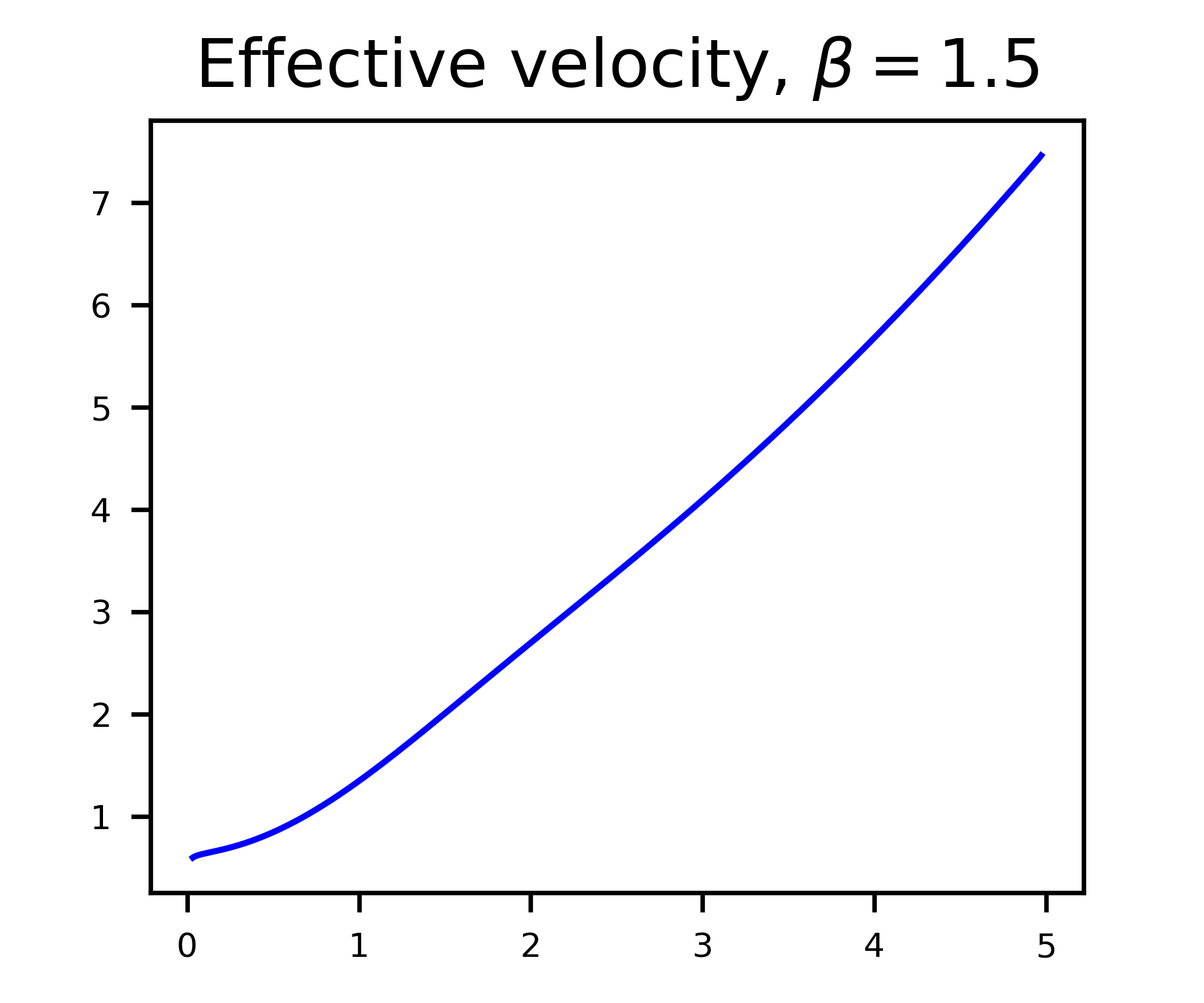
Figure 1: $v_{\textrm{eff}}$ for $\beta=1.5$, $V(x)=\frac{x^{2}}{2}$

6 Numerical Results

In this section, we present the numerical results that we obtained, in the last part of this section we present the method that we used to numerically simulate both the classical correlation functions and the GHD predictions.

6.1 Description of the results

We compared the GHD prediction of the correlation functions of the Volterra lattice with the molecular dynamics simulation for three different temperature corresponding to $\beta=1;1.5$, see figure 2.

In each of these cases, we have evaluated the GHD approximations (also called Landau-Lifshitz approximation) ${\mathtt{S}}(x,t)$ (5.6) of the correlators for all $0\leq n\leq m\leq 1$ using the numerical scheme that we describe in 6.2.2. Their graphs are displayed in Figures 2 as dashed black lines. The colored lines represent the molecular dynamics simulations. According to the ballistic scaling predicted in (5.6), we plot $tS_{m,n}(j,t)$ as a function of $j/t$ for $t=200,400,600$. Here the values of $S_{m,n}(j,t)$ is approximated using the numerical scheme that we describe in section 6.2.1.

The agreement between the molecular dynamics simulation and the prediction of the GHD is astonishing for negative values of $\xi=\frac{x}{t}$, but for positive values of such parameter the GHD prediction does not capture the oscillation of the correlation functions. The main reason is that the relation $\xi=-\frac{v_{\textrm{eff}}(w)-q_{1}}{\kappa_{\beta}}$ is not a bijection between ${\mathbb{R}}$ and ${\mathbb{R}}_{+}$, thus the prediction of the GHD develop a singularity at $\xi_{0}=-\frac{v_{\textrm{eff}}(0)-q_{1}}{\kappa_{\beta}}$ , which is exactly where the molecular dynamics simulations show an highly oscillatory behavior. For this reason, we believe that one has to consider some extra diffusive terms when approximating (5.2) in order to get a more precise description of the correlation functions for this model, as it is described in [37]. Specifically, we believe that at the point $\xi_{0}$ the diffusive effects are not a sub-leading correction to the transport dynamics, but they are of the same order.

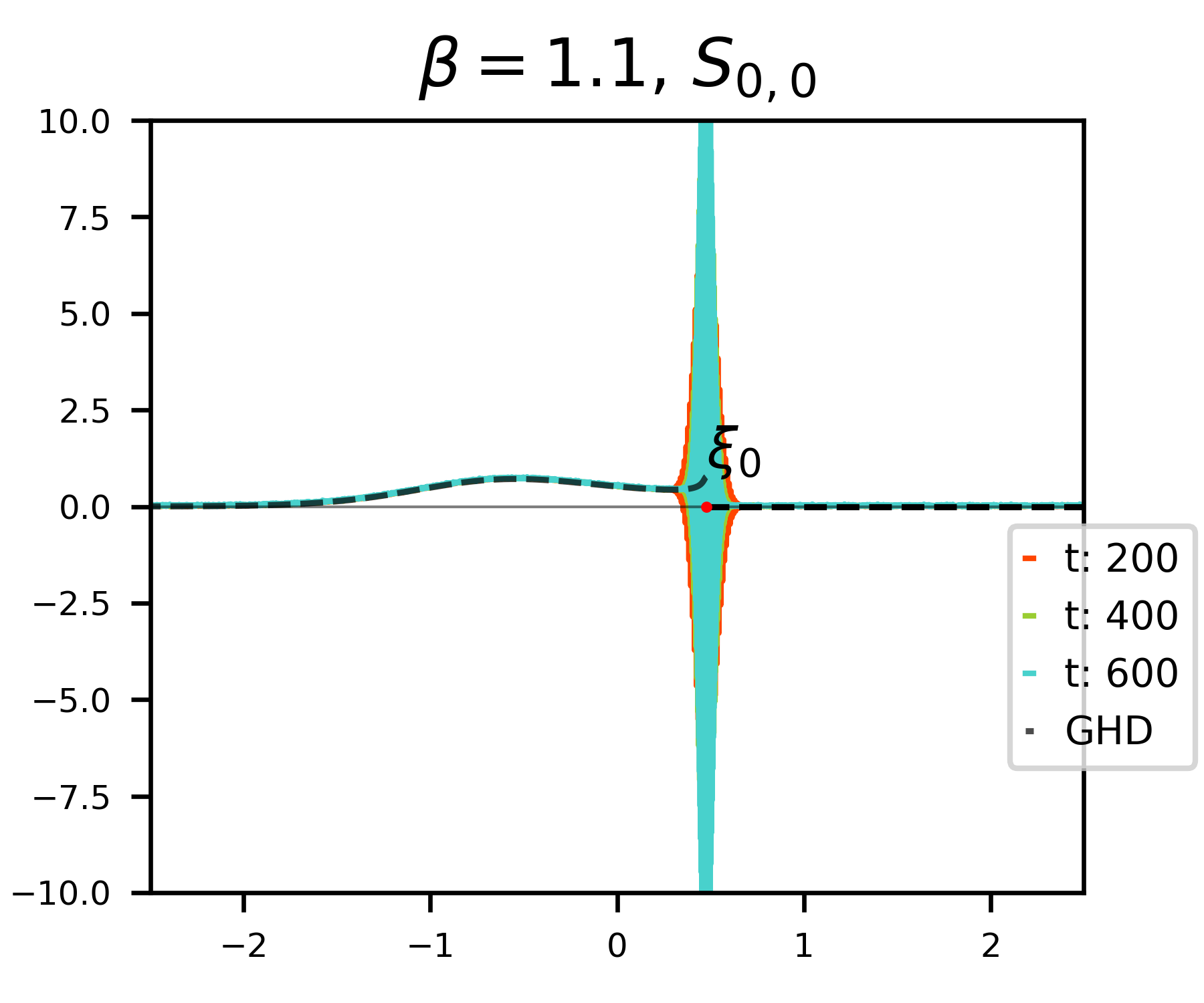
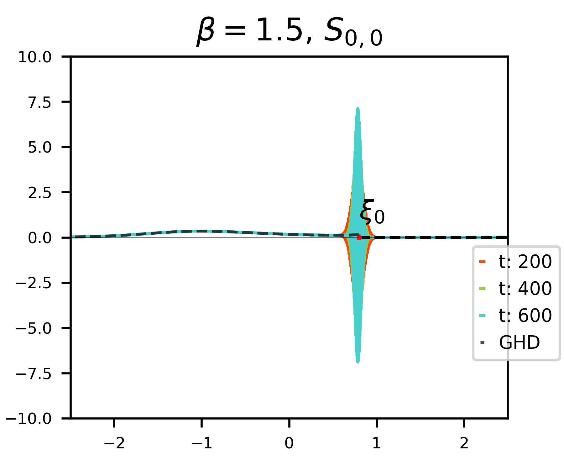
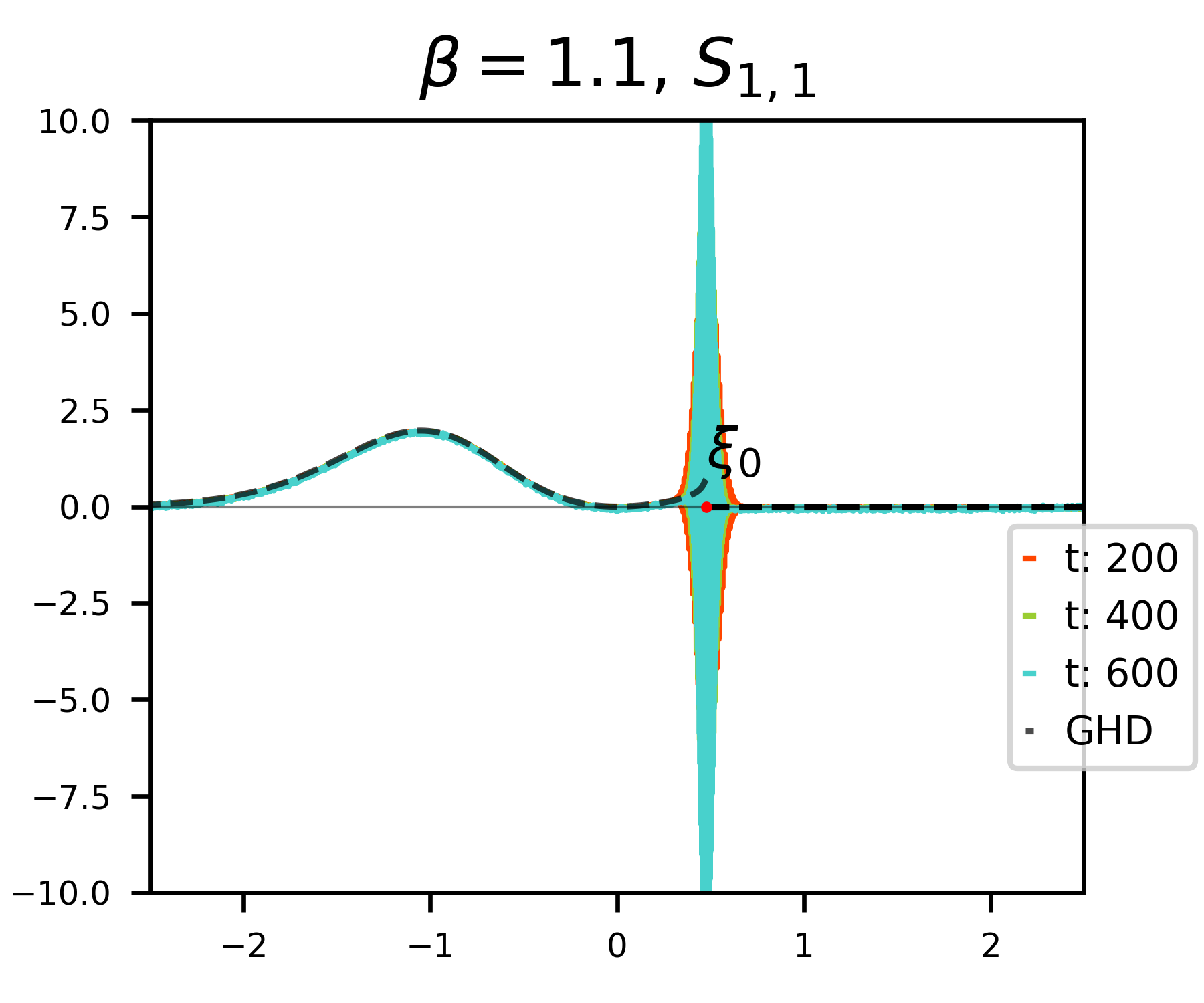
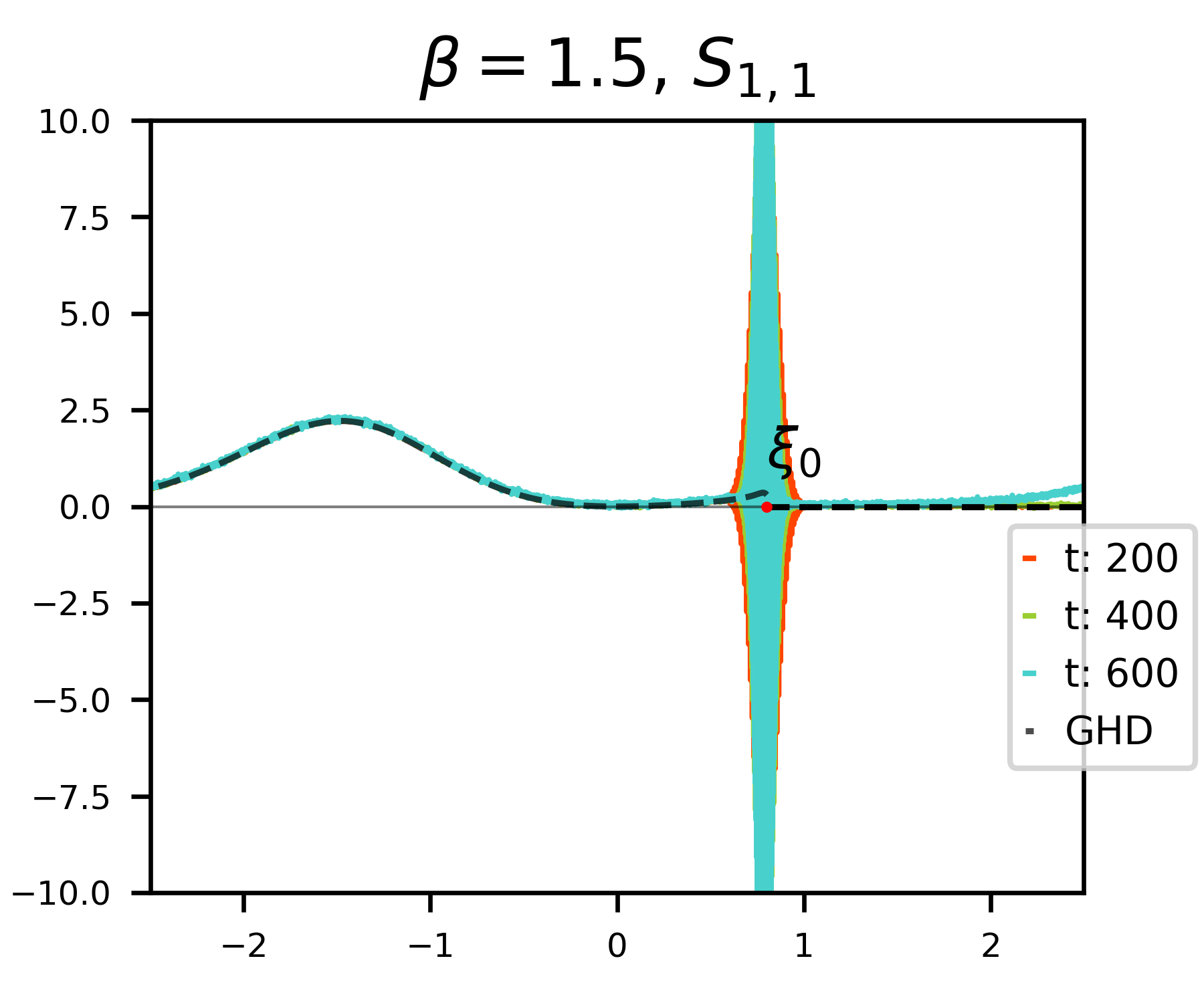
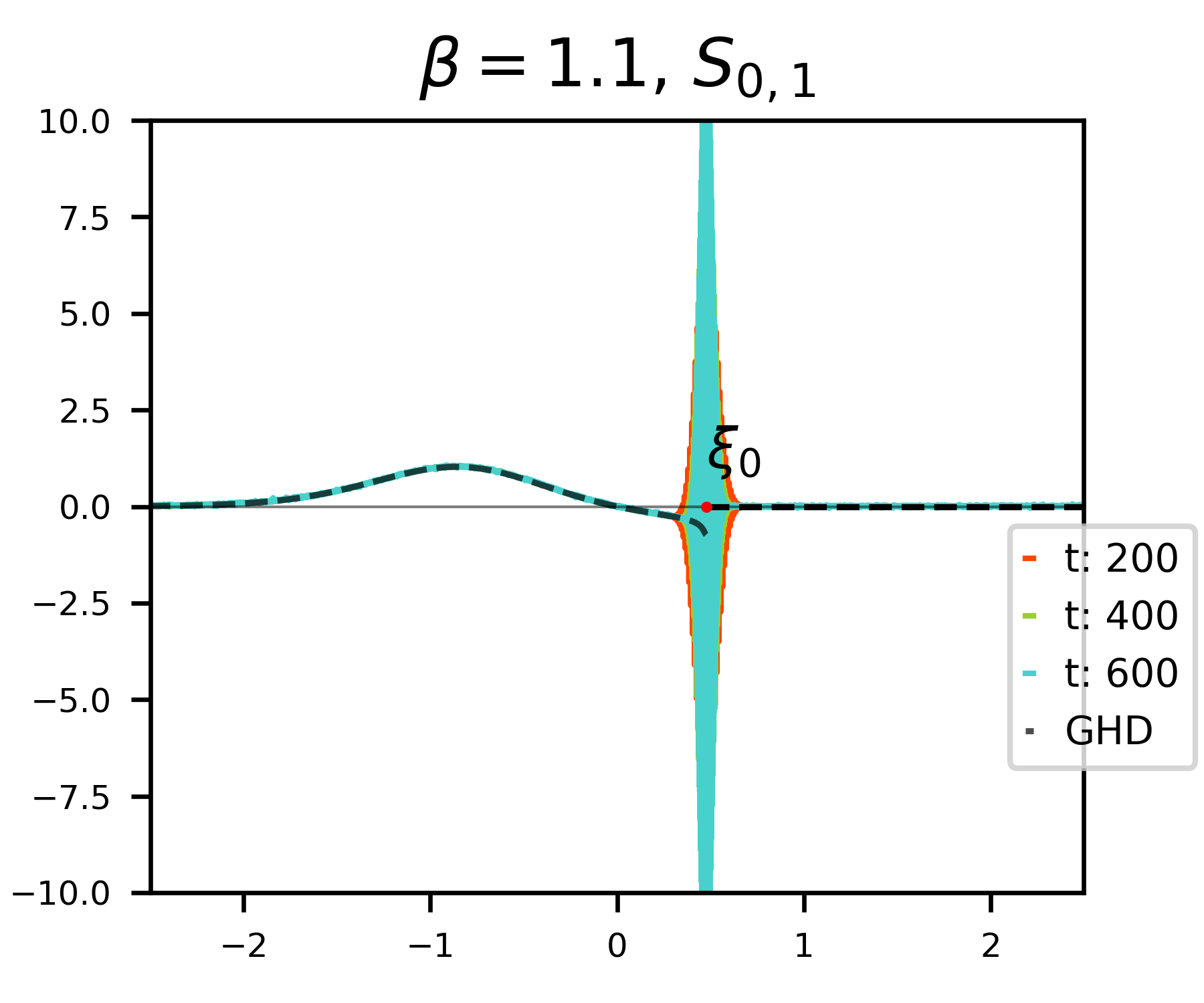
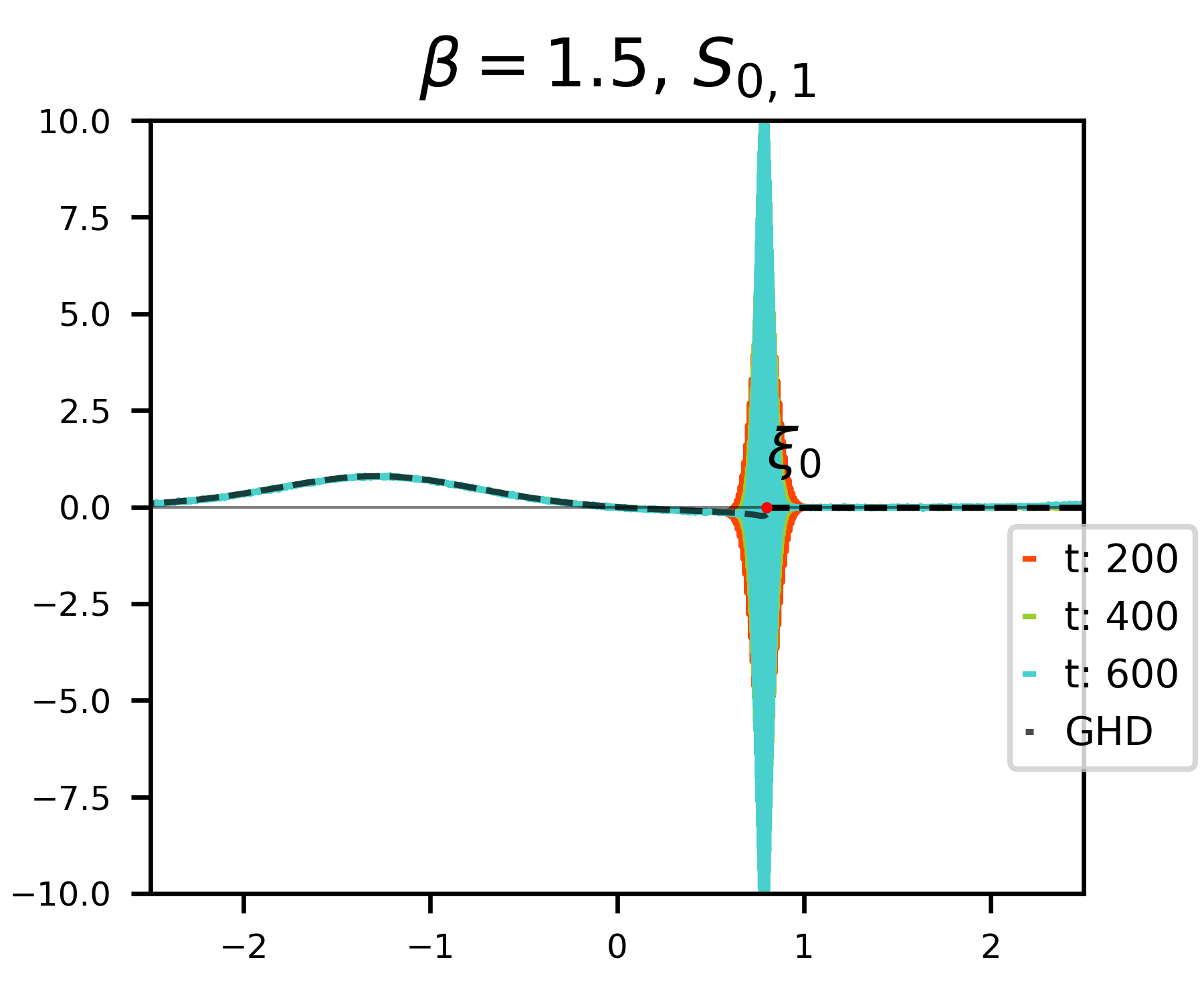
Figure 2: Volterra correlation functions: GHD predictions vs molecular dynamics simulation. Left panels: number of particles: $3000$, trials: $10^{6}$, $\beta=1.1$. Right panels: number of particles: $3000$, trials: $10^{6}$, $\beta=1.5$

6.2 Numerical simulation

This subsection is divided into two parts. In the first part we present the numerical scheme that we used to simulate the evolution of the Volterra lattice and to compute the correlation functions. In the second part, we present the numerical scheme that we used to compute the prediction of the Generalized Hydrodynamics.

6.2.1 Molecular dynamics simulations

We approximate the expectation value that is contained in the MD-definition of the correlations $S_{m,n}$ in equation (1.5) by a standard Rounge–Kutta method (RK45), whose implementation program is written in Python, and can be found at [30]. First, we generate the random initial conditions distributed according to the Gibbs measure, as given by (1.19) for the i.i.d. random variables $(a_{j})_{j=1}^{2N}$, which are distributed according to a scaled $\chi^{2}$ random variable. We generate this random vector with Numpy v1.23’s native function random.default_rng().chisquare [22]. Having chosen the initial conditions in such a manner, we solve equation (1.5).

For the evolution, we use a standard Rounge-Kutta algorithm of order 5 (RK45), we decided not to use the native Scipy v1.12.0’s algorithm [43], but we implemented it, in this way we could used the library Numba [27] to speed up the computations.

Our approximation for the expectation $S_{m,n}$ is then extracted from $10^{6}$ trials with independent initial conditions. Here we take the empirical mean of all trials where for each trial we also take the mean of the $N=3000$ sets of data that are generated by choosing each site on the ring for $j=0$.

We want to mention that almost all the pictures that appeared in this paper are made using the Python library matplotlib [23].

6.2.2 Solving linearized GHD

To numerically solve the linearized GHD equations, we use a numerical method similar to the one from [34, 31]. First, Eq. (3.6) is expressed in terms of Whittaker function $W_{\mu,\kappa}(z)$ [4], which is readily available in Mathematica [24]. This provides the solution to minimization problem (3.16).

Then, we use a simple finite element discretization of the $w$-dependent functions by hat functions, resulting in piece-wise linear functions on a uniform grid. After precomputing the integral operator $T$ in (4.11) for such hat functions, the dressing transformation (4.12) becomes a linear system of equations, which can be solved numerically. This procedure yields $[w^{2}]^{\mathrm{dr}}$, and subsequently $\sigma$ via (4.13) and $v_{\mathrm{eff}}$ via (4.44).

To evaluate the correlation functions in (1.36), we note that the delta-function in the integrand results in a parametrized curve, with the first coordinate (corresponding to $x/t$) equal to $-\frac{v_{\textrm{eff}}(w)-q_{1}}{\kappa}$ from (1.36), and the second coordinate equal to the remaining terms in the integrand divided by the Jacobi factor $|\frac{\mathrm{d}}{\mathrm{d}w}v_{\textrm{eff}}(w)|$ resulting from the delta-function.

References

[1]D. Benjamin, Lecture Notes On Generalised Hydrodynamics, SciPost
Phys. Lect. Notes, (2020), p. 18.
[2]T. Bonnemain, B. Doyon, and G. El, Generalized hydrodynamics of the
KdV soliton gas, Journal of Physics A: Mathematical and Theoretical, 55
(2022), p. 374004.
[3]A. Dembo and O. Zeitouni, Large deviation techniques and
applications, Springer, New York, NY, second ed., 1998.
[4]NIST Digital Library of Mathematical Functions.
http://dlmf.nist.gov/, Release 1.1.0 of 2020-12-15.
F. W. J. Olver, A. B. Olde Daalhuis, D. W. Lozier, B. I. Schneider,
R. F. Boisvert, C. W. Clark, B. R. Miller, B. V. Saunders, H. S. Cohl, and
M. A. McClain, eds.
[5]B. Doyon, T. Yoshimura, and J.-S. Caux, Soliton gases and
generalized hydrodynamics, Phys. Rev. Lett., 120 (2018), p. 045301.
[6]I. Dumitriu and A. Edelman, Matrix models for beta ensembles, J.
Math. Phys., 43 (2002), pp. 5830–5847.
[7]I. Dumitriu and P. J. Forrester, Tridiagonal realization of the
antisymmetric Gaussian -ensemble, J. Math. Phys., 51 (2010),
pp. 093302, 25.
[8]G. El, The thermodynamic limit of the whitham equations, Physics
Letters A, 311 (2003), pp. 374–383.
[9]G. A. El and A. M. Kamchatnov, Kinetic equation for a dense soliton
gas, Phys. Rev. Lett., 95 (2005), p. 204101.
[10]G. A. El, A. M. Kamchatnov, M. V. Pavlov, and S. A. Zykov, Kinetic
equation for a soliton gas and its hydrodynamic reductions, Journal of
Nonlinear Science, 21 (2010), p. 151–191.
[11]H. Flaschka, On the Toda lattice. II. Inverse-scattering
solution, Progr. Theoret. Phys., 51 (1974), pp. 703–716.
[12]P. J. Forrester, Log-gases and Random matrices, 2005.
Available at: http://www.ms.unimelb.edu.au/ matpjf/matpjf.html.
[13]P. J. Forrester and G. Mazzuca, The classical -ensembles
with proportional to : from loop equations to Dyson’s
disordered chain, J. Math. Phys., 62 (2021), pp. Paper No. 073505, 22.
[14]D. García-Zelada, A large deviation principle for empirical
measures on Polish spaces: application to singular Gibbs measures on
manifolds, Ann. Inst. Henri Poincaré Probab. Stat., 55 (2019),
pp. 1377–1401.
[15]A. Giorgilli, S. Paleari, and T. Penati, An Extensive Adiabatic
Invariant for the Klein–Gordon Model in the Thermodynamic
Limit, Annales Henri Poincaré, 16 (2014), pp. 897–959.
[16]M. Girotti, T. Grava, R. Jenkins, and K. D. T.-R. McLaughlin, Rigorous Asymptotics of a KdV Soliton Gas, Communications in Mathematical
Physics, 384 (2021), p. 733–784.
[17]T. Grava, M. Gisonni, G. Gubbiotti, and G. Mazzuca, Discrete
integrable systems and random Lax matrices, J. Stat. Phys., 190 (2023),
pp. Paper No. 10, 35.
[18]T. Grava, T. Kriecherbauer, G. Mazzuca, and K. D. T.-R. McLaughlin, Correlation functions for a chain of short range oscillators, Journal of
Statistical Physics, 183 (2021).
[19]T. Grava, A. Maspero, G. Mazzuca, and A. Ponno, Adiabatic invariants
for the FPUT and Toda chain in the thermodynamic limit, Comm. Math.
Phys., 380 (2020), pp. 811–851.
[20]T. Grava and G. Mazzuca, Generalized Gibbs ensemble of the
Ablowitz–Ladik lattice, Circular -ensemble and double confluent Heun
equation, Comm. Math. Phys., (2023), pp. 1–41.
[21]A. Guionnet and R. Memin, Large deviations for Gibbs ensembles of
the classical Toda chain, Electron. J. Probab., 27 (2022), pp. Paper No.
46, 29.
[22]C. R. Harris, K. J. Millman, S. J. van der Walt, R. Gommers, P. Virtanen,
D. Cournapeau, E. Wieser, J. Taylor, S. Berg, N. J. Smith, R. Kern, M. Picus,
S. Hoyer, M. H. van Kerkwijk, M. Brett, A. Haldane, J. F. del Río,
M. Wiebe, P. Peterson, P. Gérard-Marchant, K. Sheppard, T. Reddy,
W. Weckesser, H. Abbasi, C. Gohlke, and T. E. Oliphant, Array
programming with NumPy, Nature, 585 (2020), pp. 357–362.
[23]J. D. Hunter, Matplotlib: A 2d graphics environment, Computing in
Science & Engineering, 9 (2007), pp. 90–95.
[24]W. R. Inc., Mathematica, Version 14.0.
Champaign, IL, 2024.
[25]M. Kac and P. van Moerbeke, On an explicitly soluble system of
nonlinear differential equations related to certain Toda lattices,
Advances in Math., 16 (1975), pp. 160–169.
[26]R. Killip and I. Nenciu, Matrix models for circular ensembles, Int.
Math. Res. Not., (2004), pp. 2665–2701.
[27]S. K. Lam, A. Pitrou, and S. Seibert, Numba: A LLVM-based Python
JIT compiler, in Proceedings of the Second Workshop on the LLVM Compiler
Infrastructure in HPC, LLVM ’15, New York, NY, USA, 2015, Association for
Computing Machinery.
[28]M. Ljubotina, M. Žnidarič, and T. Prosen, Spin diffusion from an
inhomogeneous quench in an integrable system, Nature Communications, 8
(2017).
[29]G. Mazzuca, On the mean density of states of some matrices related
to the beta ensembles and an application to the Toda lattice, J. Math.
Phys., 63 (2022), pp. Paper No. 043501, 13.
[30]G. Mazzuca, gmazzuca/Correlation_Volterra: Volterra Correlation
Functions, Mar. 2024.
[31]G. Mazzuca, T. Grava, T. Kriecherbauer, K. T.-R. McLaughlin, C. B. Mendl,
and H. Spohn, Equilibrium spacetime correlations of the Toda lattice
on the hydrodynamic scale, J. Stat. Phys., 190 (2023), pp. Paper No. 149,
22.
[32]G. Mazzuca and R. Memin, Clt for ensembles at
high-temperature, and for integrable systems: a transfer operator approach,
2023.
[33]G. Mazzuca and R. Memin, Large deviations for Ablowitz-Ladik
lattice, and the Schur flow, Electron. J. Probab., 28 (2023), pp. Paper
No. 55, 29.
[34]C. B. Mendl and H. Spohn, High-low pressure domain wall for the
classical Toda lattice, SciPost Phys. Core, 5 (2022), p. 002.
[35]G. Misguich, K. Mallick, and P. L. Krapivsky, Dynamics of the
spin- Heisenberg chain initialized in a domain-wall state,
Phys. Rev. B, 96 (2017), p. 195151.
[36]J. Moser, Three integrable Hamiltonian systems connected with
isospectral deformations, Advances in Math., 16 (1975), pp. 197–220.
[37]J. D. Nardis, D. Bernard, and B. Doyon, Hydrodynamic Diffusion in
Integrable Systems., Physical review letters, 121 16 (2018), p. 160603.
[38]L. Piroli, J. De Nardis, M. Collura, B. Bertini, and M. Fagotti, Transport in out-of-equilibrium XXZ chains: Nonballistic behavior and
correlation functions, Phys. Rev. B, 96 (2017), p. 115124.
[39]H. Spohn, Ballistic space-time correlators of the classical toda
lattice, J. Phys. A, 53 (2020), pp. 265004, 17.
[40]H. Spohn, Generalized Gibbs ensembles of the classical Toda
chain, J. Stat. Phys., 180 (2020), pp. 4–22.
[41], Hydrodynamic
equations for the Ablowitz-Ladik discretization of the nonlinear
Schroedinger equation, ArXiv preprint: 2107.04866, (2021).
[42]H. Spohn, Hydrodynamic equations for the toda lattice, 2021.
[43]P. Virtanen, R. Gommers, T. E. Oliphant, M. Haberland, T. Reddy,
D. Cournapeau, E. Burovski, P. Peterson, W. Weckesser, J. Bright, S. J. van
der Walt, M. Brett, J. Wilson, K. J. Millman, N. Mayorov, A. R. J. Nelson,
E. Jones, R. Kern, E. Larson, C. J. Carey, İ. Polat, Y. Feng, E. W.
Moore, J. VanderPlas, D. Laxalde, J. Perktold, R. Cimrman, I. Henriksen,
E. A. Quintero, C. R. Harris, A. M. Archibald, A. H. Ribeiro, F. Pedregosa,
P. van Mulbregt, and SciPy 1.0 Contributors, SciPy 1.0:
Fundamental Algorithms for Scientific Computing in Python, Nature Methods,
17 (2020), pp. 261–272.