Combining Statistical Depth and Fermat Distance for Uncertainty Quantification

Abstract

We measure the Out-of-domain uncertainty in the prediction of Neural Networks using a statistical notion called “Lens Depth” (LD) combined with Fermat Distance, which is able to capture precisely the “depth” of a point with respect to a distribution in feature space, without any assumption about the form of distribution. Our method has no trainable parameter. The method is applicable to any classification model as it is applied directly in feature space at test time and does not intervene in training process. As such, it does not impact the performance of the original model. The proposed method gives excellent qualitative result on toy datasets and can give competitive or better uncertainty estimation on standard deep learning datasets compared to strong baseline methods.

1 Introduction

We consider a multi-class classification problem with the input space $\mathcal{X}$. In general, a classification model consists of a feature extractor (backbone) $\Phi_{\theta_{1}}$ and a classifier $h_{\theta_{2}}$: $f_{\theta}=h_{\theta_{2}}\circ\Phi_{\theta_{1}}$, where $\theta=\theta_{1}\cup\theta_{2}$ is the set of parameters of the model. The backbone transforms inputs into fixed-dimension vectors in the so-called feature space $\mathcal{F}$. The classifier $h$ then maps the features to predictions. In our experiments, the classification model is provided by a neural network, $h$ is a softmax layer consisting of a linear transformation and a softmax function, $\mathcal{F}$ is the output space of the penultimate layer right before the softmax layer. The model $f_{\theta}$ is trained on i.i.d. examples drawn from In-Distribution (ID) $P_{\text{in}}$. $f_{\hat{\theta}}$ denotes the trained model.

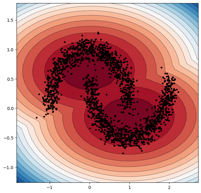
(a) Gaussian Prior

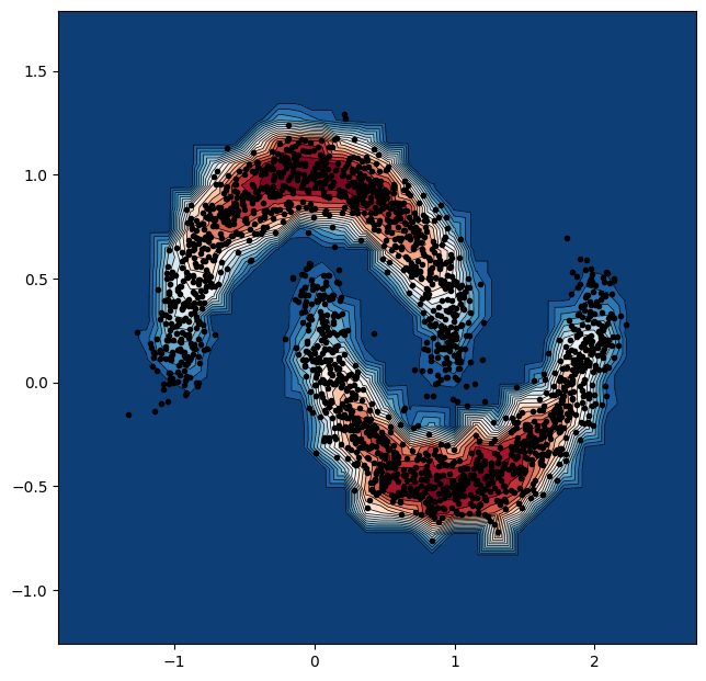
(b) Our method

Figure 1.1: Motivation example using the two-moons dataset. Colors indicate OOD score. Gaussian fitting (left), fails completely to capture the distribution of dataset whereas our proposed method (right) represents very well how central a point is with respect to (w.r.t.) clusters without any prior assumption.

OOD detection. Classification neural networks have proved highly effective in terms of precision. However, beside performance, in critical applications, one needs to detect out-of-distribution (OOD) data for safety reasons. Indeed, at the inference stage, the model should only predict for data coming from the ID and reject OOD samples. For this purpose, one needs to associate a confidence (or uncertainty) score $S$ with these data so that one can reject uncertain predictions. This is referred as Out-of-domain uncertainty (Gawlikowski et al., 2023). At the inference stage, $x$ is considered as ID if $S(x)\geq\varepsilon$ (with some threshold $\varepsilon\in\mathbb{R}$) and OOD otherwise.

We develop a method applicable directly in the feature space $\mathcal{F}$ of the trained model $f_{\hat{\theta}}$. It yields a score function $S_{\mathcal{F}}$: $S(x):=S_{\mathcal{F}}(\Phi_{\hat{\theta}_{1}}(x))$. One major advantage is that there is no need of supplementary training. Besides, the model’s performance is also preserved. Discussion about advantages of this approach over other methods is in Section 2.

A desirable property for any well-trained model is the preservation of the data geometry in the feature space.In other words, in this space, similar data should be close and dissimilar data should be far away. Intuitively, each class should be represented as a different cluster in feature space (see, e.g. Caron et al. (2018), Yang et al. (2017)). In addition, data that are dissimilar to the training data should be distant from any cluster obtained on the training data in the feature space. Assuming this desirable property, a method measuring directly “how central” a point is with respect to (w.r.t.) clusters taking into account density and geometry of each cluster in the feature space should provide an uncertainty score. For this objective, standard methods consist in assuming some prior distribution such as a Gaussian model (Lee et al., 2018). However, the assumption that the data in a cluster is Gaussian distributed or follow any particular distribution is quite restrictive. We will show in our experiments section that the Gaussian assumption fails even in a very simple case (Section 5.1). Let us take the example of a simple frame in the plane with 2 clusters corresponding to 2 classes in form of two-moons (Fig. 1.1). In this example, Gaussian fitting (Fig. 1.1a) fails totally to capture the distribution of clusters.

This motivates us to develop a non-parametric method that can measure explicitly how “central” a point is w.r.t. a cluster without the need of additional training and prior assumption. Furthermore, the method should accurately capture distribution with complex support and shape, in order to be adapted to a variety of cases. To measure how central a point is w.r.t. a distribution, we use the so-called notion of statistical Lens Depth (LD) (Liu, 1990), that will be presented in Section 3.1. Furthermore, for LD to correctly capture the shape of the distribution, an appropriate distance must be adopted that adaptively takes into account its geometry and density. Fermat distance is a good candidate for this purpose. However, it is not directly tractable as it stands on integrals along rectifiable paths. A recent paper Groisman et al. (2022) proposes the use of an explicit sampled Fermat distance and shows its consistency property (see also Cholaquidis et al. (2023)). In our work, we make use of their results to compute the LD. The general scheme is illustrated in Figure 1.2.

Figure 1.2: General scheme of our method. Given a set of features $\Phi$, the Fermat distance is a metric which respects and adapts to the distribution of $\Phi$. Lens depth wraps the Fermat distance into a probabilistic and interpretable score $S$. No additional training is needed.

Consistency of the uncertainty score. Out-of-domain uncertainty is more demanding than OOD detection. A consistent uncertainty score function should allow us to detect OOD. Furthermore, when more samples are rejected based on this score, the accuracy of the multi-class classification on the retained samples should increase. In other words, the fewer examples retained (based on the score), the better the accuracy. This means that the score represents the true confidence in prediction. Many previous methods (e.g. Sun et al. (2022), Liang et al. (2017)) focus purely on OOD detection, and this second desired property is not satisfied or proved. In contrary, we show in Sections 5.2 and 5.3 that our method respects this property. This is because our method measures a natural ”depth” of the considered example. Consequently, the larger the depth of this example, the more typical this point is (relative to the training set), and so the easier it is for the model to classify.

In summary, our contribution is at the following three levels:

• We are bringing to machine learning the mathematical tool of $LD$, combined with Fermat distance. It proves particularly efficient for OOD uncertainty quantification. We also propose improvements that avoid undesirable artifacts, and simple strategies for reducing significantly the complexity in computing $LD$.

• The method we propose is non-parametric and non-intrusive. We do not have priors on the distribution of data nor features. We do not require modifying the training algorithms.

• The method is almost hyperparameter-free, as we show that it is rather insensitive the only parameter used to define Fermat distance.

Tables 5.1 and 5.2 in the experiments section give benchmarks. And our code can be shared upon request.

2 Related Work

One approach to construct a confidence score consists in fine-tuning the model $f_{\hat{\theta}}$ using some auxiliary OOD data so that the ID and OOD data are more separable in the feature space (Liu et al., 2020). One may even use very particular type of model and training mechanism for the original classification task such as RBF models (LeCun et al., 1998) in DUQ method (Van Amersfoort et al., 2020) or Prior Networks in which the prior distribution is put on on the output of the model (Malinin & Gales, 2018). More laborious method to handle uncertainty in neural network is its Bayesian modeling ( MacKay (1992), Gal et al. (2016)). Another approach is to train some additional models to train such Deep Ensembles (Lakshminarayanan et al., 2017) or LL ratio (Ren et al., 2019). In these approaches, one needs to carefully perform the supplementary training. Otherwise one could reflect wrongly the true underlying distribution. Moreover, the performance of the multi-class classification task could be impacted. Furthermore, the training process itself contains some stochastic factors (e.g. mini-batch sampling), that could increase the error of the confidence score. For all these reasons, these methods can be considered intrusive.

Independently from above methods, a non-intrusive approach is to work directly in the feature space $\mathcal{F}$ of the trained model $f_{\hat{\theta}}$. This is non-intrusive in the sense that there is no need of supplementary training. Besides, model performance is not impacted. One of the simplest method is to use the $k$-nearest neighbor distance (Sun et al., 2022). It is very simple but has the drawback of completely ignoring cluster geometry and density. A more sophisticated approach uses minimum Mahalanobis distance (Mahalanobis, 2018) based on Gaussian prior (Lee et al., 2018). Despite taking the distribution into account, Gaussian modeling is too restrictive as it leads to an ellipsoid for shaping each cluster. A classical non-parametric method is one-class SVM (Schölkopf et al., 1999) which demands supplementary training. Besides, its effectiveness is known to be significantly influenced by the kernel choice and its hyper-parameters. On the other hand, our method needs no additional training and has following properties at the same time: (1) non-intrusive; (2) non-parametric; (3) nearly hyperparameter-free. All these properties make it unique in comparison to other methods.

3 Background

3.1 Lens Depth

Lens depth (LD) (Liu, 1990) is a specific notion of a more general quantity called Depth (Tukey, 1975). A depth is a score measure of the membership of a point w.r.t. a distribution in a general space. The greater the depth, the more central the point is to the distribution. LD of a point w.r.t a distribution $P_{X}$ is defined as the probability that it belongs to the intersection of two random balls. These balls are centered at two independent random points $X$ and $Y$, both having the distribution $P_{X}$ and a radius equal to the distance between $X$ and $Y$. More formally, if we work on $\mathbb{R}^{d}$, the LD of a point $x\in\mathbb{R}^{d}$ w.r.t. $P_{X}$ is defined as follows,

$$LD(x,P_{X}):=\mathbb{P}(x\in B_{1}\cap B_{2})\ .$$ (3.1)

Here

• $d$ is a given distance on $\mathbb{R}^{d}$,

• $X_{1}$,$X_{2}$ are i.i.d with law $P_{X}$,

• $B(p,r)$ is the closed ball centered at $p$ with radius $r$,

• $B_{i}=B(X_{i},d(X_{2},X_{1})),\ i=1,2$.

Let $A(X_{1},X_{2})=B_{1}\cap B_{2}$. Equation (3.1) naturally gives rise to the following empirical version of LD,

$$\widehat{LD}_{n}(x):={\binom{n}{2}}^{-1}\sum_{1\leq i_{1}<i_{2}\leq n}\mathds{1}_{A(X_{i_{1}},X_{i_{2}})}(x)\ .$$ (3.2)

Note that for the empirical version, the intersection set might be rewritten as

$$A(X_{1},X_{2})=\{x:\max_{i=1,2}d(x,X_{i})\leq d(X_{1},X_{2})\}\ .$$ (3.3)

Obviously, a crucial question is the choice of the distance $d$. A naive choice is the Euclidean one. Examples of $\widehat{LD}$ using Euclidean distance are depicted in Fig. 3.1. We see that in the Gaussian case, the level curves of $\widehat{LD}$ rather well capture the distribution. However, for the moon distribution they fail miserably. This is not surprising as the Euclidean distance does not take into account the data distribution $P_{X}$.

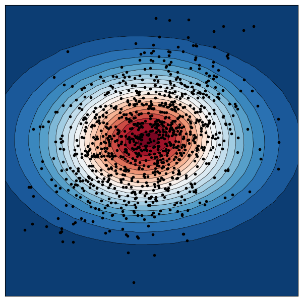
(a) Gaussian

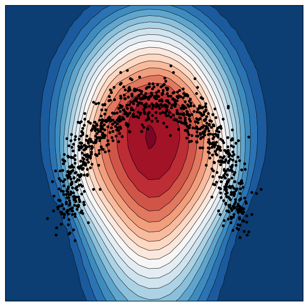
(b) Moon

Figure 3.1: $\widehat{LD}$ using Euclidean distance. We see that using simply Euclidean distance cannot capture correctly the distribution.

This gives rise to a natural problem as stated by Groisman et al. (2022): How to learn a distance that can capture both the geometry of the manifold and the underlying density? The Fermat distance allows us to solve this problem and it is presented in the following section.

3.2 Fermat distance

Following Groisman et al. (2022), let $S$ be a subset of $\mathbb{R}^{d}$. For a continuous and positive function $f:S\rightarrow\mathbb{R}_{+}$ , $\beta\geq 0$ and $x,y\in S$, the Fermat distance $\mathcal{D}_{f,\beta}(x,y)$ is defined as

$$\mathcal{D}_{f,\beta}(x,y):={\inf}_{\gamma}\mathcal{T}_{f,\beta}(\gamma)\ ,$$ (3.4)

where

$$\mathcal{T}_{f,\beta}(\gamma):=\int_{\gamma}f^{-\beta}\ .$$ (3.5)

The infimum is taken over all continuous and rectifiable paths $\gamma$ contained in $\bar{S}$, the closure of $S$, that start at $x$ and end at $y$.

Sample Fermat Distance. Let $Q$ be a non-empty, locally finite, subset of $\mathbb{R}^{d}$, serving as dataset. $|x|$ denotes Euclidean norm of $x$, $q_{Q}(x)\in Q$ is the particle closest to $x$ in Euclidean distance – assuming uniqueness. For $\alpha\geq 1$, and $x,y\in\mathbb{R}^{d}$, the sample Fermat distance is defined as:

$$D_{Q,\alpha}(x,y):=\min\Big{\{}\sum_{j=1}^{k-1}|q_{j+1}-q_{j}|^{\alpha}\ :(q_{1},\dots,q_{k})\in Q^{k}$$

$$\quad\quad\quad\text{ with }q_{1}=q_{Q}(x),\ q_{k}=q_{Q}(y),\ k\geq 1\Big{\}}\ .$$ (3.6)

Groisman et al. (2022) show that the sample Fermat distance when appropriately scaled converges to the Fermat distance.

Intuition behind Sample Fermat Distance. The sample Fermat distance searches for the shortest path relating the points. The length of each path is the sum of the Euclidean distances of consecutive points in the path powered by $\alpha$. With $\alpha=1$, the shorted path between $x$ and $y$ is simply the line relating $q_{Q}(x)$ and $q_{Q}(y)$ (Fig. 3.2a). However, with a sufficiently large $\alpha$, this definition of path length discards consecutive points with a large Euclidean distance instead favoring points that are closely positioned in terms of Euclidean distance. So, this will qualify the path passing through high density areas. Moreover, as this distance depends also on the number of terms in the sum in Eq. (3.6), this enforces a path to be smooth enough. These two remarks show that Fermat distance naturally captures the density and geometry of the data set.

In Fig. 3.2, we go back to the moon example. We randomly choose 2 points and compute the Fermat path. We see that with $\alpha=1$, we recover the Euclidean distance and so the Fermat path is simply a line. For $\alpha$ larger than 1 but not large enough (for instance, $\alpha=1.2$, Fig. 3.2b), the Fermat path still does not capture the orientation of the dataset. However, as $\alpha$ gets larger, the Fermat path rapidly tracks the orientation of the dataset. For instance, with $\alpha=3$, the path follows very well the distribution shape.

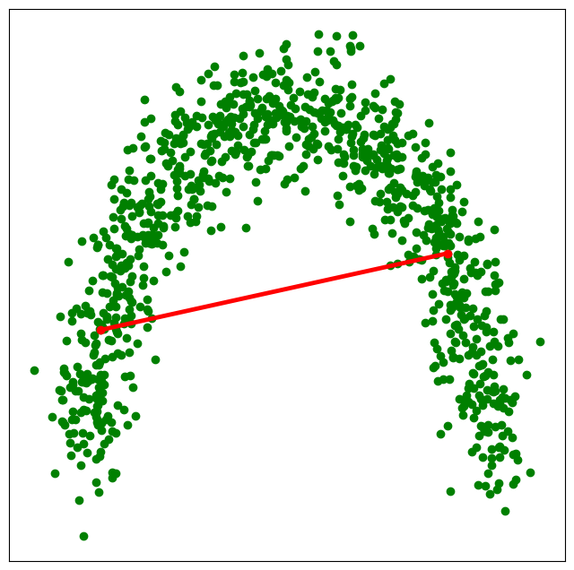
(a) $\alpha=1$

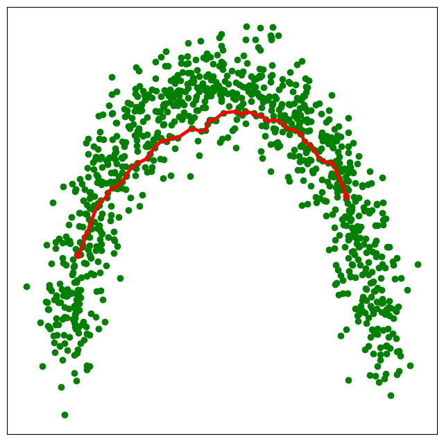
(b) $\alpha=1.2$

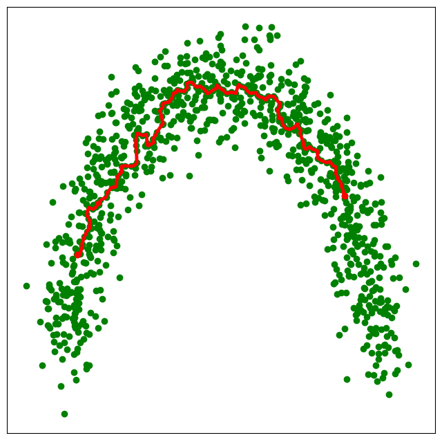
(c) $\alpha=3$

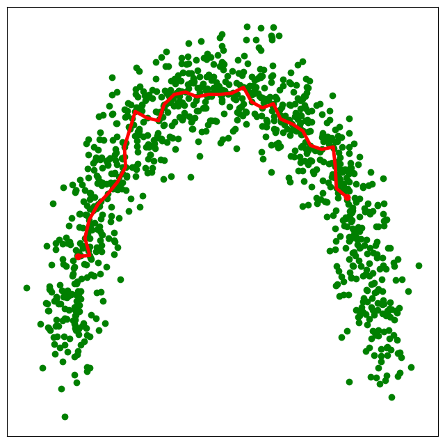
(d) $\alpha=7$

Figure 3.2: Sample Fermat path between two fixed randomly chosen points using different values of $\alpha$.

4 Combining LD and Fermat Distance

4.1 Artifacts from classical Fermat distance

In the computation of the depth, instead of using Euclidean distance, we use sample Fermat distance. The results for the moon and spiral datasets are depicted in Fig. 4.1a and 4.1b. We see that the shape of datasets is much better captured. However, we also observe some zones having constant LD value (represented by the same color). The existence of such zones are explained by the following proposition:

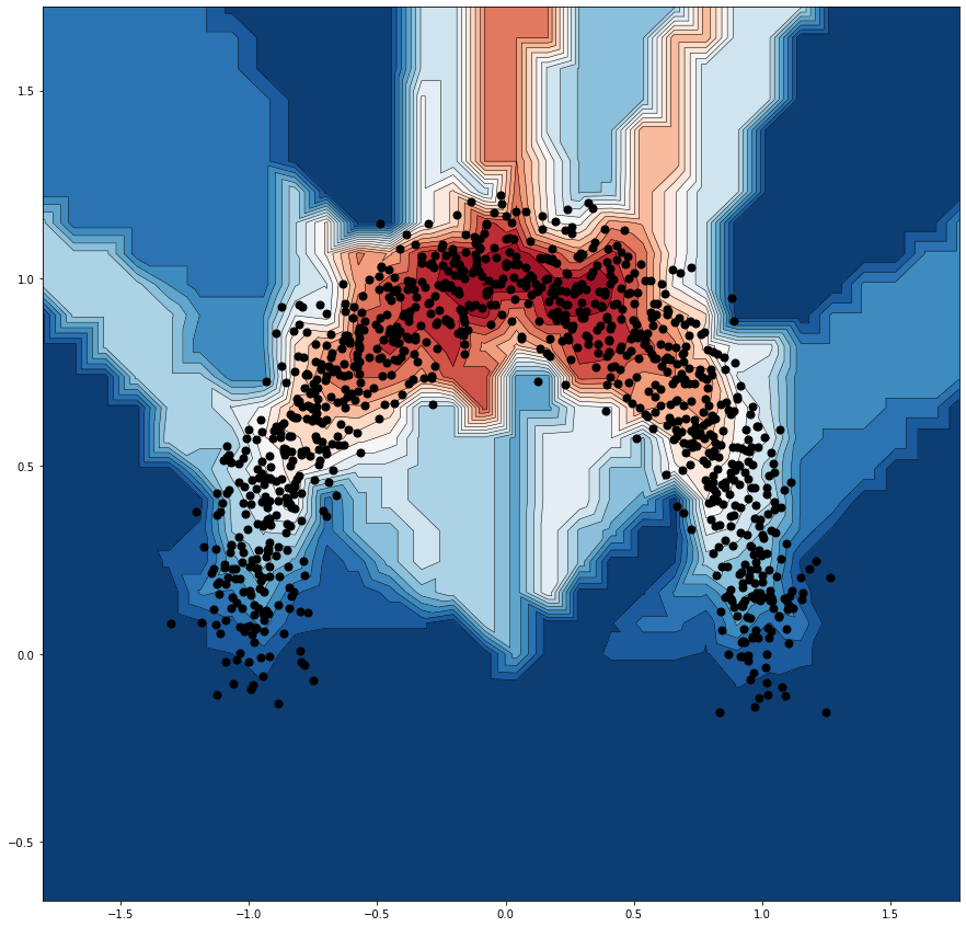
(a) Before

(b) Before

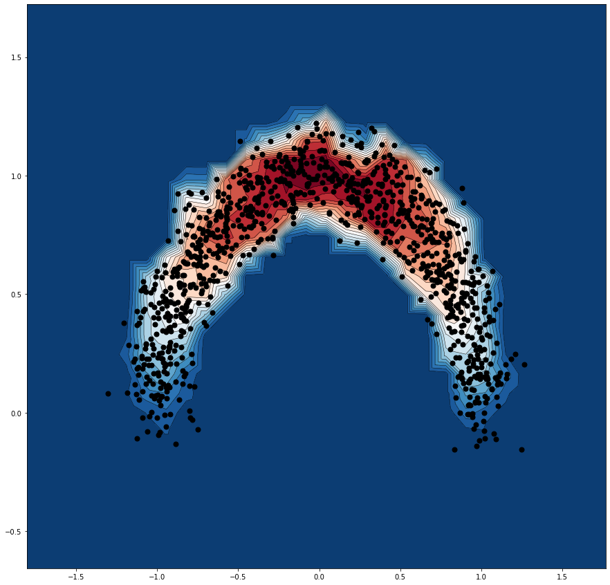
(c) After

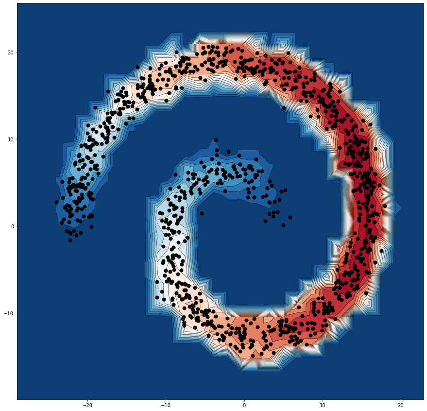
(d) After

Figure 4.1: $\widehat{LD}$ with Sample Fermat Distance on moon and spiral datasets. (a) and (b) are results of using directly sample Fermat distance in Eq. (3.6). This produces undesirable artifacts where we observe zones of constant value of $LD$. This phenomenon is explained by Proposition 3. (c) and (d) use our modified version in Eq. (4.1): it captures perfectly the distributions.

Proposition 1.

For $x\in\mathbb{R}^{d},\;\widehat{LD}(x)=\widehat{LD}(q_{Q}(x))$. In other words, the empirical lens depth is constant over the Voronoï cells associated to $Q$.

The proof of Proposition 3 is in Appendix C. The consequence of the last proposition is that, even for a point far removed from $Q$, the value of $\widehat{LD}$ remains the same as that of its nearest point in $Q$. Consequently, $\widehat{LD}$ does not vanish at infinity. This is totally undesirable, as an ideal property of any depth is to vanish at infinity. To avoid this undesirable artifact, we need to modify the sample Fermat distance so that it takes into account the distance to $Q$.

4.2 Modified Sample Fermat Distance

The modified distance is defined, for $y\in Q,\;x\in\mathbb{R}^{d}$ as follows:

$$D^{\mathrm{modif}}_{Q,\alpha}(x,y):=\min_{q\in Q}\{|x-q|^{\alpha}+D_{Q,\alpha}(q,y)\}\ .$$ (4.1)

Here, $D_{Q,\alpha}(q,y)$ has been defined in Eq. (3.6).

Interpretation. In the original definition in Eq. (3.6), the path always starts by the closest point in the dataset. Consequently, the distance to this closest point is totally ignored. To eliminate this drawback, the distance to a potential starting point lying in $Q$ is added. Note that the optimization problem for calculating $D^{\mathrm{modif}}_{Q,\alpha}$ is of the same type as that for calculating $D_{Q,\alpha}$ with only a change of starting point. Hence, the consistency of this empirical distance towards the theoretical Fermat distance remains true. Indeed, in the new formulation (4.1), the point $q\in Q$ is not fixed at $q_{Q}(x)$ but remains free and is a part of the optimization problem. Notice further that our modified version enjoys two nice properties. Firstly, if $x\in Q$ then Eq. (4.1) coincides with Eq. (3.6) ($D^{\mathrm{modif}}_{Q,\alpha}(x,y)=D_{Q,\alpha}(x,y)$). Secondly, $D^{\mathrm{modif}}_{Q,\alpha}(x,y)$ increases to infinity when $x$ is going far away from $Q$. Consequently, in this case, the corresponding $\widehat{LD}$ w.r.t $Q$ tends to $0$. The $\widehat{LD}$ using this modified version of the distance is displayed on two examples in Fig. 4.1c and 4.1d. With our modification, the undesirable artifact of constant-valued zone is erased. Furthermore, for points far away from the dataset, $\widehat{LD}$ tends quickly to 0. In conclusion, our method captures the shape of distributions perfectly.

4.3 Qualitative evaluation of stability

We experiment and evaluate the stability of our method on the spiral dataset. This is a tricky dataset, and a standard method like the Gaussian one cannot capture its shape.

4.3.1 Stability with respect to number of training points

When running a statistical algorithm, it is desirable to have as large a sample as possible. However, in many cases, only a very small amount of data is available. This motivates the study of the stability of our method in a small data regime. Here, we simulate the spiral dataset with 1000 points. Then, we choose randomly only $20\%$ of the simulated points (i.e. 200 points) as the sample dataset to compute $LD$. We perform different runs for different random samples with $\alpha=5$ for a visual evaluation. For the sake of brevity, only the results of four tests are shown in Fig. 4.2. More replications are displayed in Appendix B. We see that in the 4 tries, our method gives slightly different estimation of $LD$. This small fluctuation is to be expected, as we take only $20\%$ of the points at random each time. Nevertheless, the method captures the shape of the data set really well (the full sample of 1000 points is displayed in the figures).

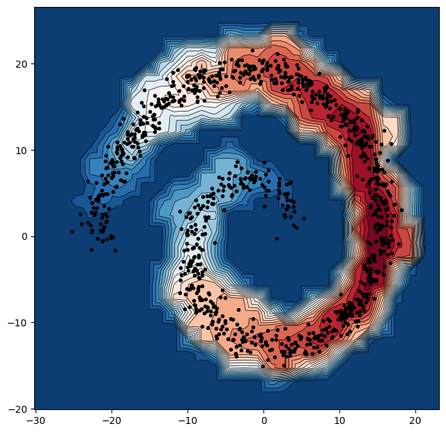
(a) $1^{st}$ try

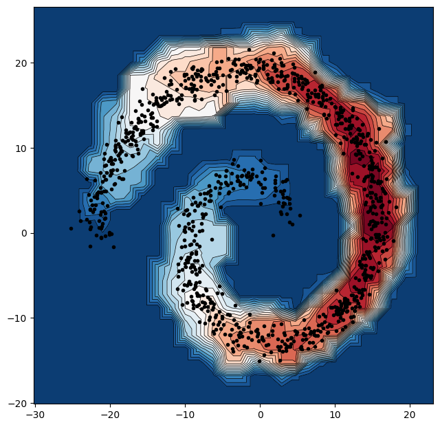
(b) $2^{nd}$ try

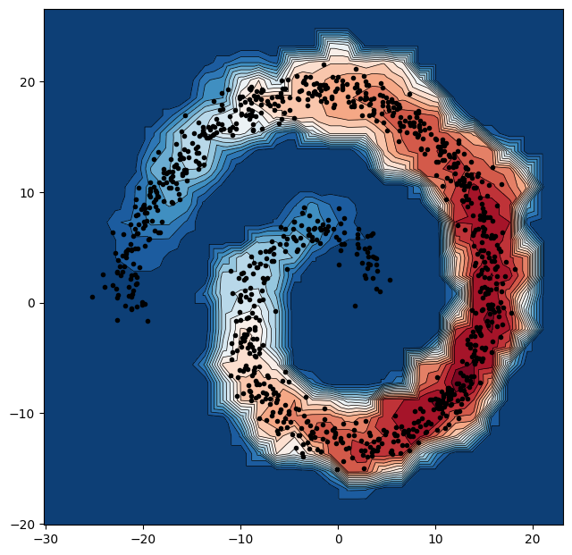
(c) $3^{rd}$ try

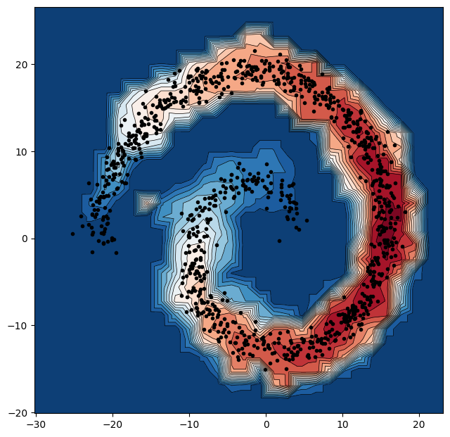
(d) $4^{th}$ try

Figure 4.2: $LD$ using only $20\%$ of points (200 points) on simulated spiral dataset of 1000 points. The contours of $LD$ level changes slightly between different tries, but in general, the proposed method captures well the general shape of distribution.

4.3.2 Stability with respect to the hyperparameter $\alpha$

In our method, only one hyperparameter ($\alpha$), governing the Fermat distance needs to be chosen. It is therefore important to assess the stability of the method w.r.t. $\alpha$. For this purpose, we experiment with different values of $\alpha>1$ (recall that $\alpha=1$ corresponds to the Euclidean distance). For each $\alpha\in\{3,5,10,15\}$, we test our method on the spiral dataset. Results are shown in Fig. 4.3. The conclusion is that our method is very stable through different values of $\alpha$. Indeed, in the 4 cases, it always captures almost perfectly the dataset support, which implies a strong stability of the method. Of course this stability is only achieved in the proper range when $\alpha$ is large enough (See Fig. 3.2).

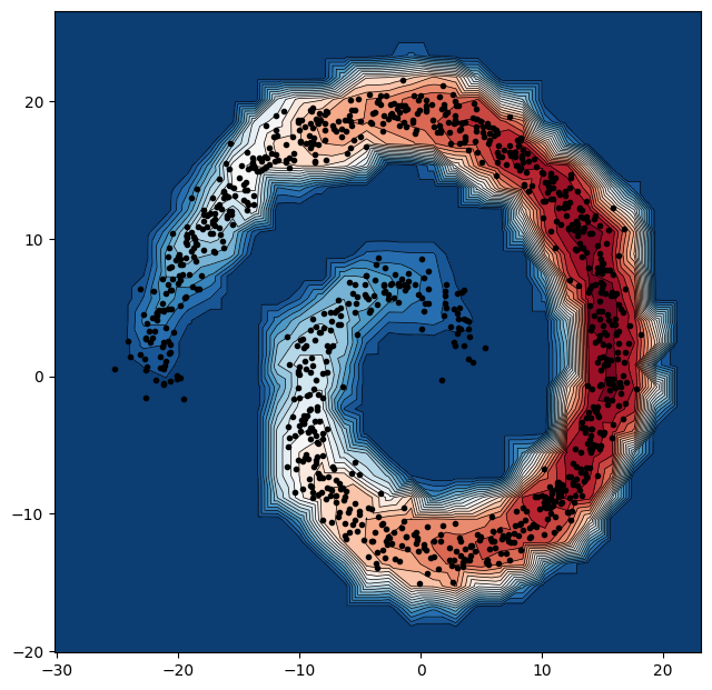
(a) $\alpha=3$

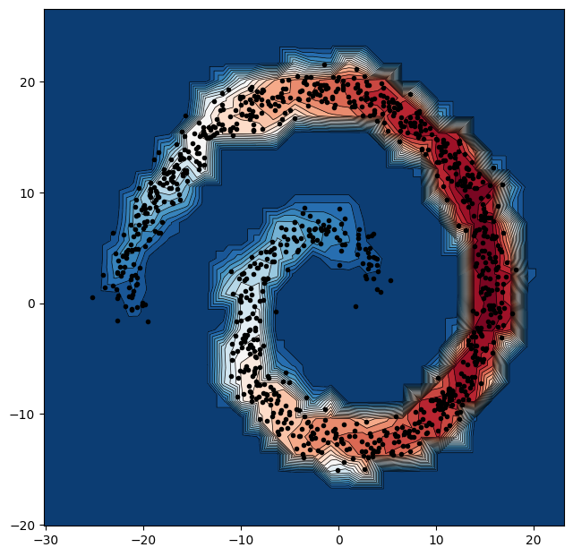
(b) $\alpha=5$

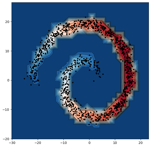
(c) $\alpha=10$

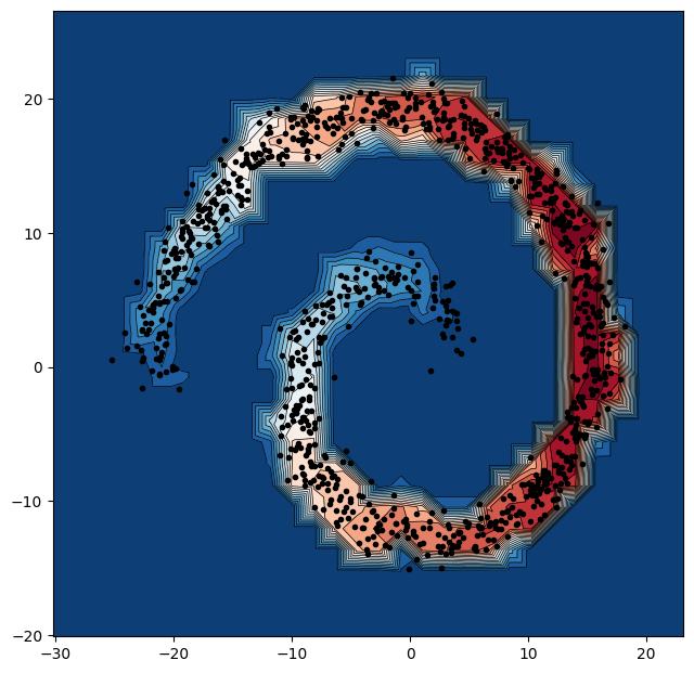
(d) $\alpha=15$

Figure 4.3: $LD$ applying different values of hyperparameter $\alpha$ in Sample Fermat Distance. For different values of $\alpha$, the method always captures really well the distribution.

4.4 From LD to OOD uncertainty score

Our ultimate objective is to use $LD$ to provide an out-of-distribution uncertainty score. To do so, we apply $LD$ to the feature space $\mathcal{F}$ of our classification model. Let $C$ be the number of separate clusters. Now, there are two ways for computing $LD$ of a new point: (1) All the clusters are considered as a sole distribution to compute $LD$; (2) Compute $LD$ w.r.t. the different clusters and then take the $max$ among the $LD$’s (i.e. $LD$ w.r.t. the nearest cluster). It turns out that the first approach gives unsatisfying result as explained in Appendix D. So, we adopt the second approach in this paper. More formally, let us denote $\widehat{LD}(\Phi(x),\mathcal{C}_{i})$ the empirical LD of $x$ w.r.t. the $i^{th}$ cluster formed by training examples of class $i$ (in the feature space). Then, the confidence score of $x$ is defined as

$$S(x):=\max_{i}\widehat{LD}(\Phi(x),\mathcal{C}_{i})\ .$$ (4.2)

4.5 Reducing complexity for computing $LD$

From Eq. (3.2), we can deduce that the complexity of calculating $LD$ for a given point is more than $O(CN^{2})$ ($C$ is the number of classes, $N$ is number of examples in each class). It is therefore very interesting to reduce the number of inner points $N$ used to calculate $LD$ while maintaining good precision. Keeping only $n$ inner points among the $N$ initial ones, we then have 3 different straightforward strategies:

• I. Random. Randomly sample without replacement $n$ points among $N$ intial points.

• II. K-mean/center. We want the $n$ points to cover well the support of the initial sample. Hence, we first apply a K-mean clustering with $n$ centroids on the $N$ points. Then, the $n$ resulted centroids are used as inner points.

• III. K-mean/center+. Same as strategy II, but instead of using directly the centroids, we use the inner point closest to each centroid.

We test and discuss about these strategies in Appendix E. It turns out that K-mean / Center outperforms the two other strategies with a very small number of inner points $n$. Indeed, K-mean / Center has a regularization effect from averaging points (for calculating centroids). We conjecture that this effect makes the method much more stable, and also facilitates the capture of the overall shape of the cluster by avoiding certain irregular points that could have a negative impact on the estimate of $LD$. We refer to Appendix E for more discussion and detailed experiment. So, for the rest of this paper, we use strategy K-mean / Center.

5 Experiments on Neural Networks

We first evaluate our method on the two-moon dataset. Then, we evaluate on 2 benchmarks FashionMNIST/MNIST and CIFAR10/SVHN the ability of our method for the detection of Out-of-distribution. Besides, we also evaluate the consistency property of our uncertainty score as presented in introduction section (shown in Fig. 5.2 and 5.3). Without further mention, we fix $\alpha=7$ for all experiments.

Experiment Setup: For a fair comparison, we use the same model architectures as in the previous work of Van Amersfoort et al. (2020) for the two experiments FashionMNIST/MNIST and CIFAR10/SVHN. More details about the models and the training schemes can be found in the Appendix A. Moreover, as in Van Amersfoort et al. (2020), at test time, we use the statistics (mean and standard deviation) of the training set (i.e. FashionMNIST or CIFAR10 in our case). Indeed, these statistics are used both in the Batch normalization layers and in the data normalization process (both for OOD and for ID set).

5.1 How is the input distribution represented in the feature space of softmax model?

We apply our method on the feature space $\mathcal{F}$ of softmax model with the assumption that the input distribution is properly represented in $\mathcal{F}$. To assess this assumption, we first perform experiment on the two-moon dataset consisting of 2 classes, each having a moon shape. We train a neural network with 2 hidden layers for classification. After training, the model parameters are fixed and different methods for uncertainty evaluation are applied in $\mathcal{F}$.

One popular way to provide an uncertainty score is to use the predictive distribution entropy. It is maximized when the distribution is uniform. In this example, predictive distribution entropy is high only in a boundary zone (Fig. 5.1f). This is to be expected, as the model is trained to learn a boundary between the two classes. Nevertheless, it is desired to assign a high uncertainty to the region without training data. Indeed, it might be too risky to make decision in these zones, especially in critical applications.

Is Gaussian prior suitable? We consider the methods of Euclidean distance (Fig. 5.1d) and Mahalanobis distance (Fig. 5.1e). For the Euclidean distance method, we compute the distance to the centroids of the different clusters (in $\mathcal{F}$) and then we take its minimum. For the Mahalanobis distance method we proceed in the same way but using the metric based on the covariance matrix. Surprisingly, in this example, the crude use of Euclidean distance seems to better capture the input distribution than the use of the Mahalanobis distance (failing miserably on this dataset). This suggests that the distribution of clusters in feature space is more complicated than the Gaussian one.

This remark shows the necessity to have a method able to capture better the distribution. $LD$ can capture impressively well the zone where we have training data (Fig. 5.1a, 5.1b and 5.1c corresponding to $\alpha=3,\,10$ and $15$). Hence, $LD$ is able to pin down clusters with a complex support shape in feature space. Furthermore, we intentionally use 3 values for $\alpha$ with large gaps to show the stability w.r.t. $\alpha$.

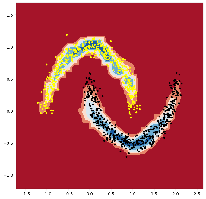
(a) LD,$\alpha=3$

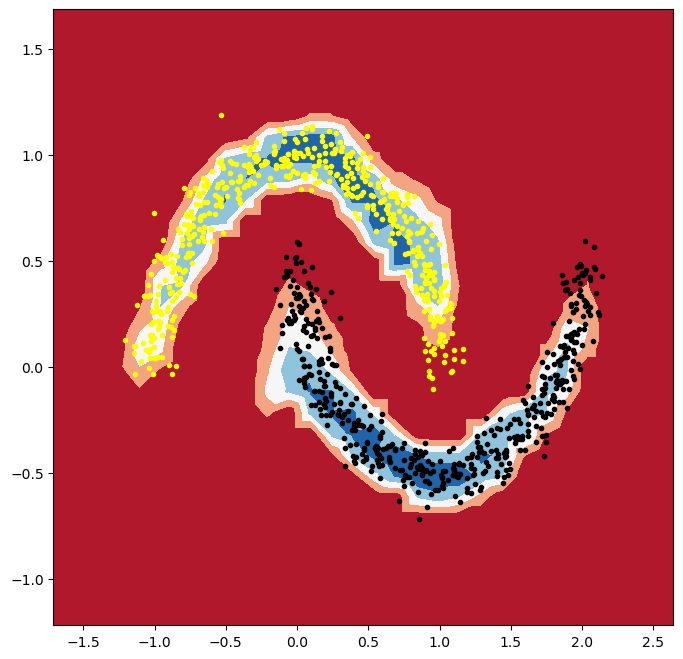
(b) LD,$\alpha=10$

(c) LD,$\alpha=15$

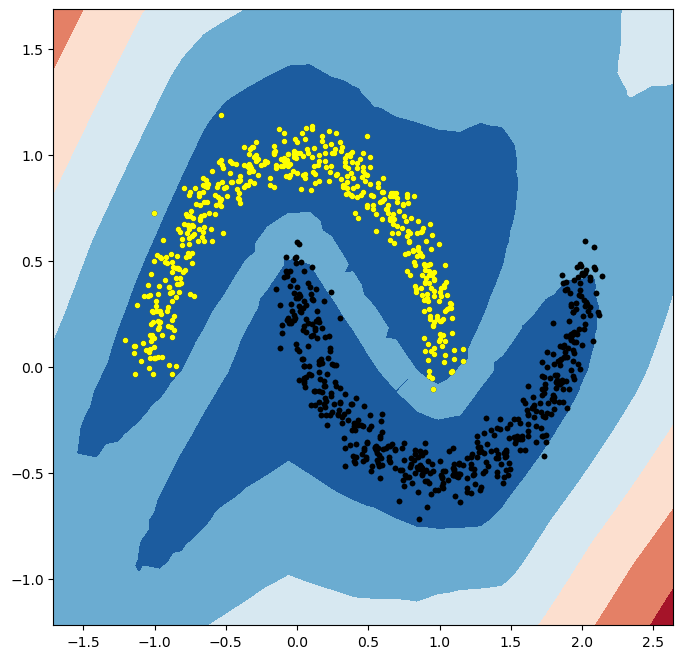
(d) Euclidean

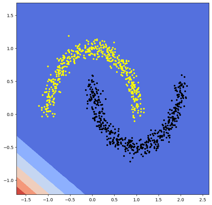
(e) Mahalanobis

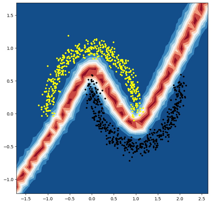
(f) Entropy of predicted probability

Figure 5.1: Methods for uncertainty estimation applied on the same neural net trained to classify 2 classes in moon-shape (represented by yellow and black points respectively). Uncertainty estimations are computed based solely on the feature space of the model without seeing directly the inputs. Our method (Fig. 5.1a, 5.1b and 5.1c) gives excellent results and much better than other methods.

5.2 FashionMNIST vs MNIST

We perform five different runs to train classification models on the data set FashionMNIST (Xiao et al., 2017).

Firstly, we evaluate our method by studying the separation capacity between the test set of FashionMNIST and of MNIST (LeCun, 1998) based on AUROC score. Results are reported in Table 5.1. We first compare our method to Euclidean and Mahalanobis distance method (Lee et al., 2018) (that are explained in Section 5.1). Notice that our method outperforms these two distance-based methods. Notice also that Euclidean distance gives slightly better AUROC score than Mahalanobis one. This might result from the fact that the distributions are far to be Gaussian, confirming once again that Gaussian assumption does not hold. A more sophisticated method called DUQ stands on a devoted neural architecture (RBF network) (see (Van Amersfoort et al., 2020)). This particular type of model is much more difficult to train and so generally does not preserve the accuracy of the main classification task (compared to standard softmax models). Once again, our method outperforms this method. This indicates that our method measures a natural “depth” directly in the feature space without the need of changing completely the model as in DUQ method. Another popular method is Deep Ensembles in which one trains and applies many independently-trained models for the same task. Consequently, this approach needs more resource both at training and inference times. Despite its heavy demanding of resource, our method outperforms this approach in this experiment. A more advanced method for density estimation is LL ratio (Ren et al., 2019). In this method, one needs to train two supplementary generative models to estimate distributions. A first model is trained on ID data and a second one is trained on perturbed inputs. This method needs an adequate noise in the way that the perturbed inputs contain only background information. Moreover, one needs to really carefully train these 2 generative models so that they can reflect the true underlying input density. With this complex process, this method gives better AUROC score than ours (in this experiment). However, we will show that our method outperforms it in the next experiment.

Table 5.1: Results on FashionMNIST, with MNIST as OOD set. Results marked by ($\Box$) are extracted from Ren et al. (2019) and ($\triangle$) are extracted from Van Amersfoort et al. (2020). Deep Ensembles by Lakshminarayanan et al. (2017), Mahalanobis Distance by Lee et al. (2018), LL ratio by Ren et al. (2019), DUQ by Van Amersfoort et al. (2020).

Charateristics	Method	AUROC
No impact on original model	LD (our method)	$0.971\scriptstyle\pm 0.001$
	Euclidean Distance	$0.943\scriptstyle\pm 0.009$
	Mahalanobis Distance ($\Box$)	0.942
Use particular type of model difficult to train	DUQ ($\triangle$)	0.955
Need to train many models	Deep Ensembles (5 Models) ($\triangle$)	0.861
Need to train extra generative models	LL ratio ($\triangle$)	0.994

Consistency curve. Next, we evaluate the usefulness of our uncertainty estimation for decision making. Following some previous works (e.g. Lakshminarayanan et al. (2017), Van Amersfoort et al. (2020)), we compound test set of FashionMNIST and MNIST together and all the data from MNIST are considered to be incorrectly predicted by the model. Then, a certain percentage of data is rejected based on their $LD$. If $LD$ is an appropriate indicator for prediction uncertainty, then accuracy on the retained data has to be an increasing function of the rejection percentage. We call the resulted curve consistency curve. The results for five runs are depicted in Fig. 5.2. We see that the curves are always increasing over 5 runs. Hence, $LD$ is a good measure for uncertainty estimation. Moreover, the 5 curves are very similar. This implies the stability of our method.

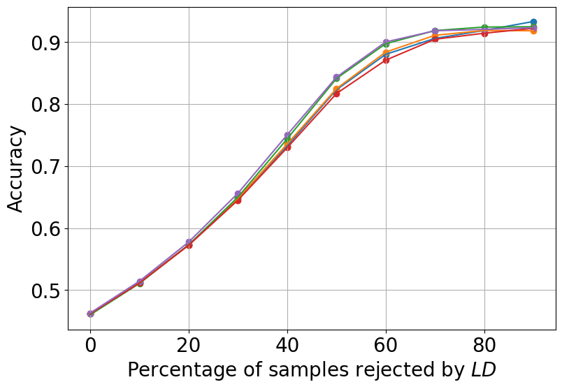
Figure 5.2: Consistency curve FashionMNIST/MNIST for 5 runs (each curve corresponds to an independently trained model).

5.3 CIFAR10 vs SVHN

We perform the same study as in the previous experiment. Nevertheless, this time we train the model on the training set CIFAR10 (Krizhevsky et al., ) and then we test on the test sets of CIFAR10 and of SVHN (Netzer et al., 2011). AUROC scores are reported in Table 5.2. We see that our method outperforms the other baseline methods. Especially, this time our method outperforms Deep Ensembles with 3 and 5 models that are costly to train. In addition, our method also outperforms the LL ratio method, although this last method requires the careful training of two additional generative models only for density estimation, which is a difficult task in itself. This reinforces our intuition that we can work directly in the feature space of the base model (i.e. the model for the main classification problem), rather than to fit supplementary models just for density estimation.

Table 5.2: Results on CIFAR10, with SVHN as OOD set. Our method outperforms other baseline methods. Results marked by ($\Box$) are extracted from Van Amersfoort et al. (2020) and ($\triangle$) extracted from Sun et al. (2022). Deep Ensembles by Lakshminarayanan et al. (2017), LL ratio by Ren et al. (2019), DUQ by Van Amersfoort et al. (2020), Energy by Liu et al. (2020), KNN by Sun et al. (2022).

Extra data	Intrusive	Method	AUROC
	No	LD (our method)	$\mathbf{0.936}\scriptstyle\pm 0.006$
	Yes	DUQ ($\Box$)	$0.927\scriptstyle\pm 0.013$
	Yes	Deep Ensembles (3 models) ($\Box$)	$0.926\scriptstyle\pm 0.010$
No	Yes	Deep Ensemble (5 models) ($\Box$)	$0.933\scriptstyle\pm 0.008$
	Yes	LL ratio ($\Box$)	0.930
	Yes	Energy($\triangle$)	0.912
Yes	No	KNN (ours)	$0.926\scriptstyle\pm 0.002$

In the Energy method (Liu et al., 2020), the authors show that softmax model is a special case of Energy-based model (LeCun et al., 2006). Based on this insight, one can derive energy from logits of softmax layer and then use the energy as a criteria to distinguish ID from OOD data. However, one needs to carefully tune the model using supplementary OOD data to increase the margin of energy between ID and OOD data. In this experiment, our method outperforms this method. This implies that capturing distribution in the feature space using our method is more effective than working on the logits of softmax layer despite its interpretation form energy-based point of view.

More recently, deep nearest neighbors method was proposed by Sun et al. (2022) (denoted as KNN in Table 5.2). In this method, one first computes the (Euclidean) distance of the considered point to all the training points in the feature space (after normalizing the features using $l^{2}$-norm). Then, the distance to the $k^{th}$ nearest neighbor is the criteria to distinguish ID from OOD data. $k$ is a hyperparameter chosen based on a validation process using an auxiliary OOD data. The AUROC score in the original paper is $0.959$. However, when we apply this method on our trained models (over 5 runs), our method outperforms this method (Table 5.2). As the 2 methods are applied in the same feature space, it would be fair to say that our method can capture better the distribution than KNN method. This is not surprising, since this method is rather heuristic and not based on clear statistical or probabilistic foundations, whereas ours is based on well-developed statistical notion which is LD.

Next, we plot the consistency curve for the 5 runs with the combined test set of CIFAR10 and of SVHN, where the data in SVHN test set are considered incorrect. (Fig. 5.3). Once again, accuracy is always an increasing function of the rejected percentage of the data based on $LD$. This confirms again that $LD$ is an appropriate indicator for uncertainty estimation and so it is useful for decision making.

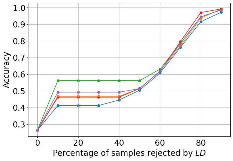
Figure 5.3: Consistency curve CIFAR10/SVHN for 5 runs (each curve corresponds to an independently trained model).

6 Discussion

In this work, we aim to show that with a sharp enough method for capturing the distribution in the feature space, we should have access to an appropriate indicator for uncertainty estimation. In the two-moon example where we train a model for classification, Euclidean and Mahalanobis distances (i.e. Gaussian fitting) fail to capture the input distribution (Fig. 5.1d and 5.1e). So, one could have conjectured that the feature space itself cannot conserve the input distribution. However, when applying our method, the input distribution is totally captured and perfectly represented (Fig. 5.1a and 5.1b). This indicates that the problem does not reside in the properness of the feature space itself but in the methods capturing the distribution. Through more challenging examples on FashionMNIST/MNIST and CIFAR10/SVHN, we once again confirm this last statement as our method gives AUROC scores that are competitive or better than those of other methods.

In some prior works, one makes ID and OOD data more separable in the feature space by applying techniques such as: performing some preprocessing techniques on the inputs (e.g. Liang et al. (2017), Lakshminarayanan et al. (2017)); fine-tuning neural net using OOD data (e.g. Liu et al. (2020)); applying some particular loss function on the feature space (e.g. Sun et al. (2022)). These techniques are orthogonal to our method and so they can be combined with ours. Hence, these techniques are not considered here. Indeed, we aim to highlight the importance of the method capturing the distribution. Combining these techniques with our method is out-of-scope of this paper and will be studied in a future work.

7 Conclusion

In this work, we use the statistical notion of Lens Depth combined with a modified version of the sample Fermat distance. This combination captures naturally the shape and density of the input distribution. This is not the case with many previously proposed methods, which assume a prior distribution or use additional models with trainable parameters, or even modify the mechanism of the training process. Our method is non-parametric and non-intrusive. Through a toy dataset as well as experiments conducted on Deep Neural Networks, we show that our method adapts very well to many cases. Hence, our work is opening new tracks for non-parametric methods capturing the input distribution to quantify uncertainty in the context of Deep Learning. For future work, it would be interesting both to have an efficient algorithm for computing Lens Depth with some error bound and to investigate more the impact of the hyper-parameter $\alpha$.

Finally notice that, while we were focused on neural networks, any classification model with a feature space, e.g. kernel methods, can benefit from our framework.

Appendix A Experimental Details

All experiments related to neural networks are implemented in Pytorch 2.0.1+cuda, with its default initialization.

A.1 Two-moons

For generating two-moon dataset, we use package scikit-learn (Pedregosa et al., 2011), with noise 0.07, random state 1, and 1000 samples.

For model, we construct a simple fully connected network with 2 hidden layers, each gives output of dimension 20. First hidden layer is followed by non-linearity ReLU. We train model for 160 epochs using Adam optimizer, learning rate $10^{-3}$, other parameters are set by default of Pytorch package.

A.2 FashionMNIST

For a fair comparison, we follow exactly the same CNN architecture proposed in (Van Amersfoort et al., 2020) and the same training scheme with only one minor modification: the dimension of penultimate layer is 25 instead of 256 for efficient computation related to LD. We observe this modification has no impact on accuracy of model. We refer reader to (Van Amersfoort et al., 2020) for details. From training set, we randomly split 80:20 to have training data and validatation. We choose the best model based on accuracy on validation set. Test accuracy after training over 5 runs is $92.35\%\pm 0.19$.

For estimating $\widehat{LD}$, we use 1500 training examples for each class based on results of the experiment in Section E. We observed that applying the method on normalized feature vectors (L2-norms) (which is the reported result) gives slightly better result than applying directly on the feature vectors. The method is applied on the test set of FashionMNIST consisting of 10,000 images and the test set of MNIST also consisting of 10,000 images).

A.3 CIFAR10

We use ResNet-18 model implemented by (DeVries & Taylor, 2017) with a minor modification and training scheme of the same authors. More specifically, after Global Average Pooling layer of CNN, we add a layer of output dimension of 25 instead of 256 proposed by (Van Amersfoort et al., 2020) before softmax layer. For training model, we use SGD optimizer with nesterov momentum, learning rate 0.1 (decayed by factor of 5 at epochs 60,120 and 160), momentum 0.9, weight decay $5\cdot 10^{-4}$.Model is trained for 200 epochs. We train model on the full training set (i.e. no validation set) and save the last model, i.e. the model at epoch 200. Test accuracy after training over 5 runs is $0.950\pm 0.001$.

As there are many more images to test compared to the previous experiment, we use only 1000 training images in each class for estimate $LD$ using K-mean/Center strategy to have a reasonable run time. We tested the method on normalized and non-normalized feature vectors and observed no significant difference. The reported result is on non-normalized vectors. Notice that the method is applied on test sets of CIFAR10 consisting of 10,000 images and of SVHN consisting of 26,032 images.

Appendix B More qualitative results of Fermat Lens Depth on spiral dataset using $20\%$ points

We use $LD$ using only $20\%$ of points (200 points) on simulated spiral dataset of 1000 points over 10 runs for qualitatively evaluating stable of the method w.r.t. number of points.Results in Fig.B.1.

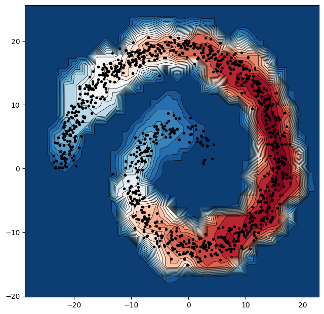
(a) $1^{st}$ try

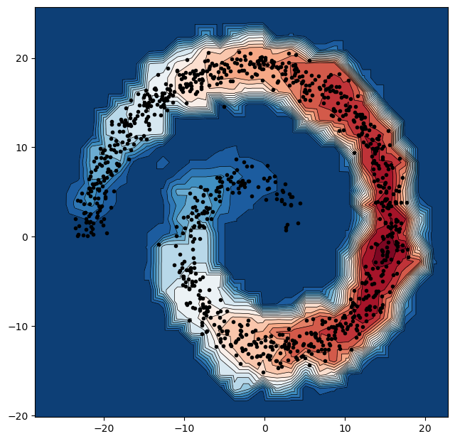
(b) $2^{nd}$ try

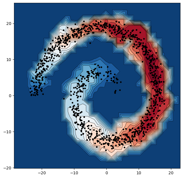
(c) $3^{rd}$ try

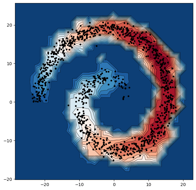
(d) $4^{th}$ try

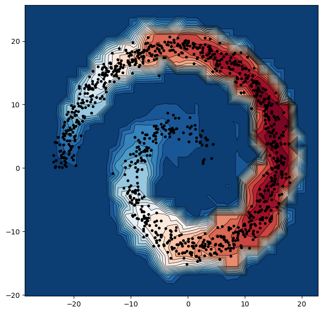
(e) $5^{th}$ try

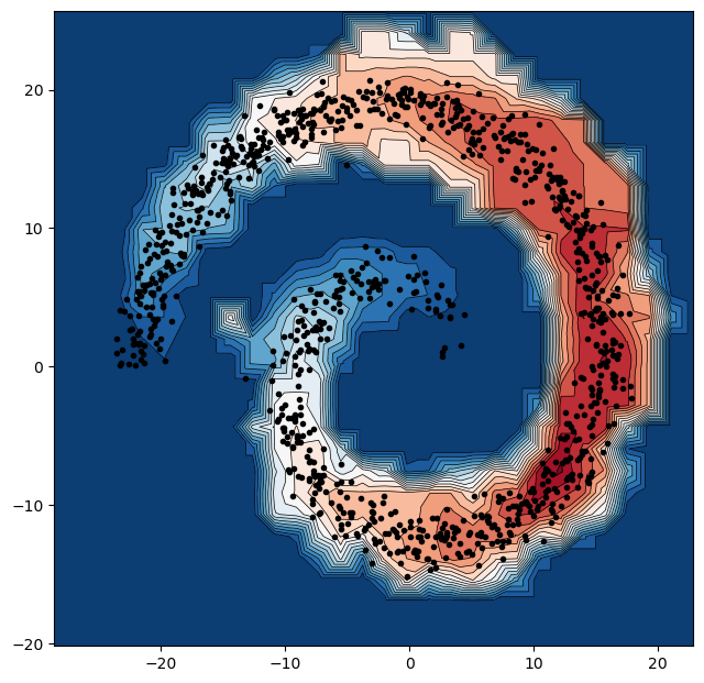
(f) $6^{th}$ try

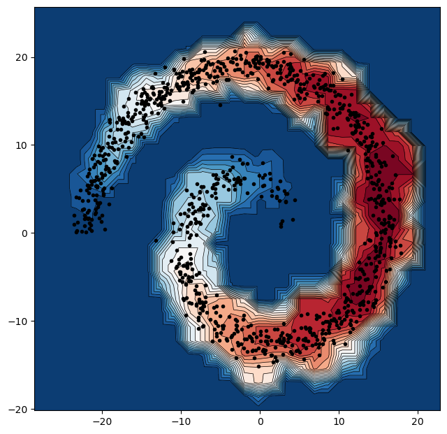
(g) $7^{th}$ try

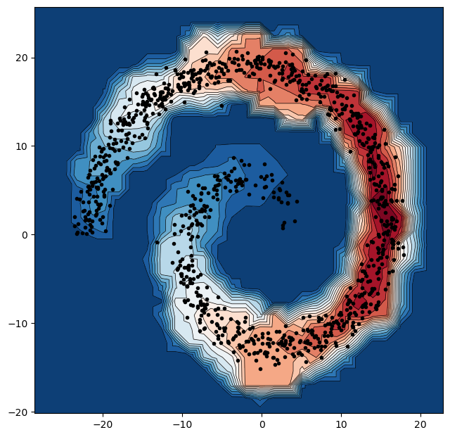
(h) $8^{th}$ try

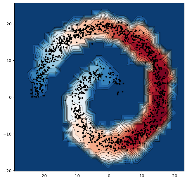
(i) $9^{th}$ try

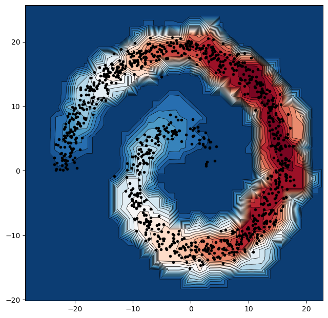
(j) $10^{th}$ try

Figure B.1: $LD$ using only $20\%$ of points (200 points) on simulated spiral dataset of 1000 points over 10 runs. We see that the contours of $LD$ level changes slightly between different tries, but in general, the proposed method captures well the general form of distribution. Note that the points presented in the plot are the full dataset of 1000 points.

Appendix C Proof of Proposition 1

Proof.

By definition, $q(q(x))=q(x)$ and $q(y)=y$ as $q(x),y\in Q$, so the closest point to them in $Q$ is themselves. Hence, according to Eq.3.6, it is obvious that $D_{Q,\alpha}(x,y)=D_{Q,\alpha}(q(x),y),\forall x\in\mathbb{R}^{d}\quad\text{and}\quad y\in Q$. Applying this sample Fermat distance to Eq.3.2 to compute empirical $LD$, we obtain $\widehat{LD}(x)=\widehat{LD}(q(x))$. ∎

Appendix D One or multiple clusters?

Our ultimate objective is to use $LD$ for finding out-of-distribution data associated with an uncertainty (or equivalently confidence) score. For this purpose, we apply $LD$ in feature space of softmax model. More concretely, we apply in the activation of penultimate layer right before softmax layer. In this setup where we have different separate clusters, one important question is: Can we simply consider them as one distribution for computing LD?

To answer this question, we simulate a dataset composed of 3 separate Gaussian clusters and then we compute $LD$ w.r.t this dataset by consider them as one distribution. The result is shown in Fig.D.1a. We see that the result is not good: value of $LD$ is large for zones lying between clusters whereas in this case, we want $LD$ to be large only in 3 cluster and NOT in the zones lying between them. So, the solution for this problem is quite straightforward: we compute $LD$ of a points w.r.t different clusters, than the final $LD$ of that point is considered as its $LD$ w.r.t to the closest cluster, i.e. we take the max among computed $LD$’s. The result is shown in Fig.D.1b. We see that the result now is much bette: $LD$ is only large in the zones of dataset which are 3 clusters.

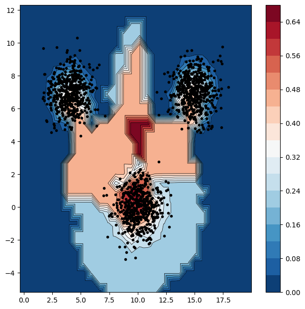
(a) Consider 3 clusters as one distribution

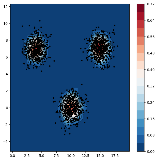
(b) Max of $LD$ w.r.t to different clusters

Figure D.1: $LD$ computed by 2 ways: (a)Consider 3 clusters as one distribution w.r.t which one compute $LD$ and (b) Compute $LD$ w.r.t 3 separate clusters than final $LD$ is computed as the max among the 3 $LD$’s computed

Appendix E Effectiveness of Reduced Lens Depth

In this section, we evaluate the effectiveness of the 3 strategies discussed in Section 4.5 to reduce the computing complexity of $LD$. We evaluate the quality of each strategy by measuring how well the ID can be separated from OOD set in term of the AUROC metric. The pair FashionMNIST/MNIST is used to assess the suitability of the three strategies. This pair is much more difficult to handle than MNIST/NotMNIST as argued in previous works (e.g. Van Amersfoort et al. (2020)). For each strategy, we use $n\in\{500,1000,1500\}$ points for each class (each class contains 6000 training examples). Results are reported in Table E.1. In all cases, strategy II always gives the best result. Remarkably, with only 500 points, K-mean / Center is already better than the two other strategies with 1500 points. K-mean / Center has a regularization effect from averaging points (for calculating centroids). We conjecture that this effect makes the method much more stable, and also facilitates the capture of the overall shape of the cluster by avoiding certain irregular points that could have a negative impact on the estimate of $LD$.

Moreover, as number of points are increased from 500 to 1500, we observe no significant improvement in AUROC score. This reinforces our conjecture about the impact of irregular points on estimation of $LD$ and furthermore, this remark implies that if the $n$ chosen points cover well enough the initial space occupied by the $N$ original points, then we only need to choose a very small percentage of points for a good estimation of $LD$. So, for the rest of this paper, we use strategy K-mean / Center.

Table E.1: Comparing AUROC performance of strategies for reducing complexity of LD on FashionMNIST/MNIST

No. of training examples	500	1000	1500
I. Random	0.9368	0.9426	0.9436
II. K-mean / Center	0.9543	0.9548	0.9553
III. K-mean / Center+	0.9475	0.9536	0.9537

Appendix F Voronoï cells

Suppose we have a finite number of distinct points in the plane, referred as sites, seeds or generators. Each seed has a corresponding region, called a Voronoï cell, made up of all the points in the plane closer to that seed than to any other. We refer to (Aurenhammer, 1991) for more details.

References

- Aurenhammer (1991) Aurenhammer, F. Voronoi diagrams—a survey of a fundamental geometric data structure. ACM Computing Surveys (CSUR), 23(3):345–405, 1991.
- Caron et al. (2018) Caron, M., Bojanowski, P., Joulin, A., and Douze, M. Deep clustering for unsupervised learning of visual features. In Proceedings of the European conference on computer vision (ECCV), pp. 132–149, 2018.
- Cholaquidis et al. (2023) Cholaquidis, A., Fraiman, R., Gamboa, F., and Moreno, L. Weighted lens depth: Some applications to supervised classification. Canadian Journal of Statistics, 51(2):652–673, 2023.
- DeVries & Taylor (2017) DeVries, T. and Taylor, G. W. Improved regularization of convolutional neural networks with cutout. arXiv preprint arXiv:1708.04552, 2017.
- Gal et al. (2016) Gal, Y. et al. Uncertainty in deep learning. 2016.
- Gawlikowski et al. (2023) Gawlikowski, J., Tassi, C. R. N., Ali, M., Lee, J., Humt, M., Feng, J., Kruspe, A., Triebel, R., Jung, P., Roscher, R., et al. A survey of uncertainty in deep neural networks. Artificial Intelligence Review, 56(Suppl 1):1513–1589, 2023.
- Groisman et al. (2022) Groisman, P., Jonckheere, M., and Sapienza, F. Nonhomogeneous euclidean first-passage percolation and distance learning. Bernoulli, 28(1):255–276, 2022.
- (8) Krizhevsky, A., Nair, V., and Hinton, G. Cifar-10 (canadian institute for advanced research). URL http://www.cs.toronto.edu/~kriz/cifar.html.
- Lakshminarayanan et al. (2017) Lakshminarayanan, B., Pritzel, A., and Blundell, C. Simple and scalable predictive uncertainty estimation using deep ensembles. Advances in neural information processing systems, 30, 2017.
- LeCun (1998) LeCun, Y. The mnist database of handwritten digits. http://yann. lecun. com/exdb/mnist/, 1998.
- LeCun et al. (1998) LeCun, Y., Bottou, L., Bengio, Y., and Haffner, P. Gradient-based learning applied to document recognition. Proceedings of the IEEE, 86(11):2278–2324, 1998.
- LeCun et al. (2006) LeCun, Y., Chopra, S., Hadsell, R., Ranzato, M., and Huang, F. A tutorial on energy-based learning. Predicting structured data, 1(0), 2006.
- Lee et al. (2018) Lee, K., Lee, K., Lee, H., and Shin, J. A simple unified framework for detecting out-of-distribution samples and adversarial attacks. Advances in neural information processing systems, 31, 2018.
- Liang et al. (2017) Liang, S., Li, Y., and Srikant, R. Enhancing the reliability of out-of-distribution image detection in neural networks. arXiv preprint arXiv:1706.02690, 2017.
- Liu (1990) Liu, R. Y. On a notion of data depth based on random simplices. The Annals of Statistics, pp. 405–414, 1990.
- Liu et al. (2020) Liu, W., Wang, X., Owens, J., and Li, Y. Energy-based out-of-distribution detection. Advances in neural information processing systems, 33:21464–21475, 2020.
- MacKay (1992) MacKay, D. J. C. A practical bayesian framework for backpropagation networks. Neural Computation, 4:448–472, 1992. URL https://api.semanticscholar.org/CorpusID:16543854.
- Mahalanobis (2018) Mahalanobis, P. C. On the generalized distance in statistics. Sankhyā: The Indian Journal of Statistics, Series A (2008-), 80:S1–S7, 2018.
- Malinin & Gales (2018) Malinin, A. and Gales, M. Predictive uncertainty estimation via prior networks. Advances in neural information processing systems, 31, 2018.
- Netzer et al. (2011) Netzer, Y., Wang, T., Coates, A., Bissacco, A., Wu, B., and Ng, A. Y. Reading digits in natural images with unsupervised feature learning. 2011.
- Pedregosa et al. (2011) Pedregosa, F., Varoquaux, G., Gramfort, A., Michel, V., Thirion, B., Grisel, O., Blondel, M., Prettenhofer, P., Weiss, R., Dubourg, V., Vanderplas, J., Passos, A., Cournapeau, D., Brucher, M., Perrot, M., and Duchesnay, E. Scikit-learn: Machine learning in Python. Journal of Machine Learning Research, 12:2825–2830, 2011.
- Ren et al. (2019) Ren, J., Liu, P. J., Fertig, E., Snoek, J., Poplin, R., Depristo, M., Dillon, J., and Lakshminarayanan, B. Likelihood ratios for out-of-distribution detection. Advances in neural information processing systems, 32, 2019.
- Schölkopf et al. (1999) Schölkopf, B., Williamson, R. C., Smola, A., Shawe-Taylor, J., and Platt, J. Support vector method for novelty detection. Advances in neural information processing systems, 12, 1999.
- Sun et al. (2022) Sun, Y., Ming, Y., Zhu, X., and Li, Y. Out-of-distribution detection with deep nearest neighbors. In International Conference on Machine Learning, pp. 20827–20840. PMLR, 2022.
- Tukey (1975) Tukey, J. W. Mathematics and the picturing of data. In Proceedings of the International Congress of Mathematicians, Vancouver, 1975, volume 2, pp. 523–531, 1975.
- Van Amersfoort et al. (2020) Van Amersfoort, J., Smith, L., Teh, Y. W., and Gal, Y. Uncertainty estimation using a single deep deterministic neural network. In International conference on machine learning, pp. 9690–9700. PMLR, 2020.
- Xiao et al. (2017) Xiao, H., Rasul, K., and Vollgraf, R. Fashion-mnist: a novel image dataset for benchmarking machine learning algorithms, 2017.
- Yang et al. (2017) Yang, B., Fu, X., Sidiropoulos, N. D., and Hong, M. Towards k-means-friendly spaces: Simultaneous deep learning and clustering. In international conference on machine learning, pp. 3861–3870. PMLR, 2017.