The Squared Kemeny Rule for Averaging Rankings
Abstract.
Manuscript: April 2024
For the problem of aggregating several rankings into one ranking, Kemeny (1959) proposed two methods: the median rule which selects the ranking with the smallest total swap distance to the input rankings, and the mean rule which minimizes the squared swap distances to the input rankings. The median rule has been extensively studied since and is now known simply as Kemeny’s rule. It exhibits majoritarian properties, so for example if more than half of the input rankings are the same, then the output of the rule is the same ranking.
We observe that this behavior is undesirable in many rank aggregation settings. For example, when we rank objects by different criteria (quality, price, etc.) and want to aggregate them with specified weights for the criteria, then a criterion with weight 51% should have 51% influence on the output instead of 100%. We show that the Squared Kemeny rule (i.e., the mean rule) behaves this way, by establishing a bound on the distance of the output ranking to any input rankings, as a function of their weights. Furthermore, we give an axiomatic characterization of the Squared Kemeny rule, which mirrors the existing characterization of the Kemeny rule but replaces the majoritarian Condorcet axiom by a proportionality axiom. Finally, we discuss the computation of the rule and show its behavior in a simulation study.
1. Introduction

Many search engines allow users to sort results by several criteria. For example, websites such as booking.com and expedia.com allow users to sort hotels by their price, their review score, or their distance to the city center. They also offer sorting by combinations of these criteria (for example “best reviewed and lowest price”, see Figure 1). More generally, they could allow users to specify weights over the different ways to sort alternatives (e.g. 60% price, 30% reviews, 10% location) and then present an aggregated ranking of hotels.
The task of combining several rankings (possibly with weights) into one ranking is known as rank aggregation. The best-known and most frequently discussed rule for this problem is Kemeny’s rule (Kemeny, 1959; Kemeny and Snell, 1960), which minimizes the total distance to all input rankings. To be precise, let be a set of alternatives (e.g., hotels), and let be the set of rankings (linear orders) on . For two rankings , the swap distance (or Kendall-tau distance) between them is the number of pairs of alternatives on which they disagree: . A profile is a function that assigns to each linear order a weight , with weights summing to . To aggregate the rankings in a profile into a collective ranking, we use a social preference function (SPF) , which selects for each profile a set of output rankings (ideally just one ranking, but there may be ties). Finally, Kemeny’s rule is the SPF that selects the rankings which minimize the average swap distance to the input:
Kemeny’s rule is an attractive SPF for several reasons: it is the maximum likelihood estimator (MLE) of the Mallow’s model (Young, 1988) which makes it a good fit for epistemic problems where we wish to discover a ground truth ranking given noisy estimates. Further, the rule is axiomatically characterized by a Condorcet-style axiom (Young and Levenglick, 1978); in particular, when the weight of some ranking exceeds 50%, then the output of Kemeny’s rule will be that ranking.
While this latter property is desirable in epistemic and electoral settings, for a hotel booking website it is disqualifying. In the above example of a user wishing to sort hotels by 60% price, 30% reviews, 10% location, the Kemeny output would just be the ranking by price, with review scores and location having no influence. Instead, what the user wants is a ranking where a hotel can compensate a lower position in the price ranking by a high position in the reviews and location rankings. Thus, we need a rule that faithfully follows the desired weighting, and makes use of all the information instead of ignoring low-weight criteria.
As it turns out, exactly such a rule was proposed under the name “mean rule” by Kemeny (1959) and Kemeny and Snell (1960) in the same articles that introduced Kemeny’s rule. Our name for this SPF is the Squared Kemeny rule as it is obtained by squaring the distances in the objective function:
The Squared Kemeny rule appears to have been almost entirely ignored in the subsequent literature. Young and Levenglick (1978, p. 290) quickly dismiss it, writing that “Kemeny left the problem of which solution to choose unresolved. But from the standpoint of collective decision-making there is ample reason to prefer the median, since it turns out that the median consensus leads to a Condorcet method, while the mean does not.” We believe that this dismissal was too quick.
The contribution of this paper is showing that the Squared Kemeny rule is well-suited to perform rank aggregation when we wish each input ranking to be reflected in the output ranking, to an extent that is proportional to its weight.111Proportionality can be seen as a fairness notion with respect to voters (who have a guaranteed amount of influence on the output ranking). The rank aggregation literature has studied distinct notions of fairness for candidates that come labelled as belonging to protected groups (Kuhlman and Rundensteiner, 2020; Chakraborty et al., 2022; Wei et al., 2022) Such proportionality notions have recently attracted significant attention in voting, in particular in the settings of multi-winner voting and participatory budgeting (see, e.g., Aziz et al., 2017; Lackner and Skowron, 2023; Peters et al., 2021). Following the approach in that literature, we could formalize proportionality, for example, by saying that a ranking that makes up of the weight should agree with the output ranking on at least roughly pairwise comparisons. While Squared Kemeny does not satisfy this in general, we will see that it does in important special cases, and that it satisfies an approximate version in general. More generally, we will show that Squared Kemeny behaves more like an average and thus is more responsive to changes in its input than the Kemeny rule, which behaves more like a median.
Rank Aggregation With Two Criteria
Price 90% 80% 70% 60% 50% 40% 30% 20% 10% Score
To understand how the Squared Kemeny rule behaves, it is instructive to consider the problem of aggregating just two different rankings with different weights. Let us again consider a hotel booking example. In Figure 2, we show a ranking of 6 hotels offered on booking.com in New Haven, Connecticut, for the nights 8–11 July 2024 (accessed 5 February 2024). At the very left, the hotels are ranked by price, and at the very right, they are ranked by average user score. The figure shows the output of Squared Kemeny (with ties broken consistently) when the two rankings are given different weights; the top row shows the weight given to the price ranking.
We see that Squared Kemeny smoothly interpolates between the two rankings. Indeed, the price and score rankings differ on exactly 10 pairwise comparisons, and going through the rankings from left to right, we see that in each step one pairwise swap is performed. Thus, for example, when the price ranking has weight 70% (and the score ranking has weight 30%), the Squared Kemeny ranking agrees with the price ranking on 7 of the 10 disagreement comparisons, and it agrees with the score ranking on 3 of 10.
This is true in general. We formalize this by saying that Squared Kemeny satisfies 2-Rankings-Proportionality (2RP). This axiom says that for every profile containing just two rankings , with positive weight that disagree on pairwise comparisons, we have
where is the set of one or two integers closest to . Thus, for profiles with two input rankings, the Squared Kemeny rule chooses all “mean rankings” where the number of pairwise agreements between and the input rankings is proportional to their weights.
Note that the Kemeny rule behaves very differently on profiles with two rankings – it just outputs the input ranking with higher weight.
Our main result is an axiomatic characterization of the Squared Kemeny rule that uses the same axioms as the famous characterization of the Kemeny rule by Young and Levenglick (1978), but replaces their Condorcet axiom by the 2RP axiom. We also impose a mild continuity axiom.
Theorem 3.2.
An SPF satisfies neutrality, reinforcement, continuity, and 2RP if and only if it is the Squared Kemeny rule.
Neutrality is a standard symmetry condition. The reinforcement axiom is a consistency or convexity axiom, which says that if a ranking is selected at two different profiles and , i.e., , then is also selected for all convex combinations of the two profiles (), and that in addition . This is a classic axiom that has been used in many characterizations in social choice (e.g., Young, 1975; Fishburn, 1978; Myerson, 1995; Lackner and Skowron, 2021).
Our proof operates within the space of (generalized) profiles and uses reinforcement in a standard way to obtain separating hyperplanes between the regions of profiles where some particular output ranking is selected. However, unlike Young and Levenglick (1978), we cannot pass to a lower-dimensional space of majority margins. Instead, we characterize the hyperplanes by using 2RP to construct profiles where the rule chooses rankings that form a single-crossing path, which allows us to deduce that the hyperplanes encode the Squared Kemeny rule.
General Proportionality Guarantee
The 2RP axiom applies only to profiles that contain two different rankings. Can we say anything similar about Squared Kemeny in the general case? Inspired by the literature on proportionality in multi-winner voting (Lackner and Skowron, 2023), we will consider groups of rankings and will bound the maximum distance of the output ranking to the group as a function of the group’s size.
Our first question asks how large the swap distance can be between an input ranking with weight and the output ranking of some rule , as a function of . For Kemeny, this is easy to specify: for , Kemeny might output the reverse ranking of (if this ranking has weight more than ), and so the distance can be as large as (the highest possible swap distance). When , the distance is guaranteed to be 0 by the Condorcet property of Kemeny.
For Squared Kemeny, we expect the bound to be smoother, giving some guaranteed influence to rankings with weights below . This is indeed the case. We can compute the exact worst-case bound provided by Squared Kemeny for fixed small numbers of alternatives (see Figure 3), and we can see that it is approximately linear in , except for small . We can also prove a theoretical upper bound that holds for all : the maximum distance of the Squared Kemeny output to an input ranking with weight is at most (Theorem 4.1). This bound implies that Squared Kemeny will never output the reverse ranking of an input ranking that has weight more than . For large , we prove another bound that shows this even for rankings with weight more than .
Our second question is about giving a similar type of guarantee not to a single ranking, but to a group of rankings. For example, there could be many similar rankings in the profile that each have a small weight, but which collectively have a significant weight. We want to show that the Squared Kemeny outcome cannot be too far away from those rankings, on average. Theorem 4.2 establishes a bound that applies to all groups of rankings with total weight (whether these rankings are similar or not), guaranteeing that the Squared Kemeny output has an average distance of at most to the rankings in the group, where the lower-order term vanishes quickly.
Empirical Analysis
We complement our theoretical analysis with results from simulations to better understand how the Squared Kemeny rule compares to the Kemeny rule. Since we need to compute the outcomes of the rules, we discuss their computational complexity in Section 5. In Section 6.1, we then perform a detailed analysis of an example of using the rank aggregation rules to rank cities according to a mixture of three criteria (GDP per capita, air quality, and sunniness).
Next, we analyze in Section 6.2 the rankings chosen by Kemeny and Squared Kemeny on random data. For example, we sample Euclidean profiles, where criteria and alternatives correspond to points in 2D space, and rankings are induced by sorting the alternatives by their distance to each criterion. In more detail, for the example in Figure 4, we sampled 100 profiles with 40 rankings each, where 75% of the input rankings come from a Gaussian in the lower left corner and the other 25% from a Gaussian in the upper right corner. We then computed the output rankings of the Kemeny rule (red diamonds) and of the Squared Kemeny rule (green squares), and embed these rankings in the same Euclidean space. We observe in Figure 4 that the Kemeny rule is located within the larger of the two voter clusters, while the Squared Kemeny rule interpolates between the two clusters.
Finally, in Section 6.3 we revisit our quantitative worst-case proportionality bounds from an average-case perspective, and experimentally investigate the distance between an output ranking and a group of input rankings, as a function of the total group weight. The results confirm our theoretical predictions: the Kemeny rule ensures only that large groups are satisfied, while the Squared Kemeny rule caters to all group sizes.
Applications of Proportional Rank Aggregation
Hotel booking websites are just one example where it makes sense to give users fine-grained control over how to sort items and where proportional rank aggregation methods such as Squared Kemeny are desirable. Further examples are lists of products in e-commerce (ranking by cost, rating, delivery time, etc.), newsfeeds of social networks, and database display applications in general.
There are also less technical applications, such as producing university rankings. These rankings are usually a result of aggregating rankings for several criteria (such as student satisfaction, % of students employed after graduating, research output). These rankings could be weighted and then be used to produce an aggregate ranking via Squared Kemeny as all criteria should be taken into account. Similarly, one could produce rankings of cities by livability or suitability for remote work.
In all previous examples, the input rankings are criteria (which tend to be objective) and the whole setup is essentially single-agent. However, there are also compelling multi-agent applications, where we can think of the input rankings as votes. An example might be a university hiring committee needing to rank applicants. In such a scenario, each committee member can provide their personal ranking. The output should be a ranking instead of a single winning candidate, because we do not know which candidates will accept the job offer. Proportionality may be desirable in this context to ensure that the output ranking reflects the diverse interests of the university department. Other multi-agent examples are groups of friends wanting to produce rankings of favorite music, restaurants, or travel destinations, a context in which a majoritarian method seems out of place.
In our example applications based on criteria, one may object that many criteria are numerical in nature (e.g., hotel price and average user rating). Using only the induced ranking throws away information, and taking a weighted average of the underlying numbers may produce a better result. The advantage of the rank aggregation approach is that it does not require the aggregator to decide on how to normalize the numerical values of different criteria. Normalization can be a difficult task without principled solutions – consider that hotel prices are in the hundreds while user ratings are between 0 and 10, and that for prices, lower is better, while for ratings, higher is better. Rank aggregation sidesteps these problems, and it is also more robust to outlier values.
2. The Model
Let be a finite set of alternatives. A ranking is a complete, transitive, and anti-symmetric binary relation on . We denote by the set of all rankings on . In this paper, we study the problem of aggregating rankings into a collective ranking. To this end, we define a (ranking) profile to be a function from to weights in such that . More intuitively, a ranking profile specifies for each ranking a weight; these weights may, e.g., arise from a user assigning importance to different criteria (as in the hotel example in the introduction) or represent the fraction of voters who report a ranking in an election. The restriction that the weights are rational is to ensure compatibility with electorate settings (where discrete voters report preference relations) and does not affect our results. We denote the set of all rankings profiles by . For a profile , we write for the set of rankings with positive weight.
Given a profile , we want to derive an aggregate ranking. A social preference function (SPF) does this, being a function that for every profile returns a non-empty set of chosen rankings . To help distinguish between input and output rankings, we will follow a convention of denoting the input rankings by and the output rankings by . For two rankings , their swap distance is the number of pairs of alternatives which they order differently, i.e., .
We focus on two SPFs in this paper. The Kemeny rule is defined as the set of rankings minimizing the (weighted) average swap distance between the input rankings and the output ranking, i.e., . The Squared Kemeny rule is defined analogously, but with the swap distance squared, i.e., . For a ranking , we let be its Squared Kemeny cost in .
3. Axiomatic Analysis
We begin by analyzing the Squared Kemeny rule from an axiomatic perspective. First, we demonstrate in Section 3.1 that this rule indeed behaves like an average for special profiles (profiles where only two rankings have positive weight as well as single-crossing profiles). This means that the Squared Kemeny rule is proportional on these profiles, and we use this insight to characterize this SPF in Section 3.2. Finally, we also consider standard properties such as efficiency, participation, and strategyproofness, and check which of them are satisfied by the Squared Kemeny rule in Section 3.3.
3.1. 2-Rankings-Proportionality and Single-Crossing Profiles
We start by showing that the Squared Kemeny rule is proportional in some special cases by defining two properties that formalize what it means to “proportionally” aggregate rankings on important classes of profiles. Our first property concerns cases where the rule must “average” two rankings with specified weights, just like in the introduction’s hotel example. It requires that the output ranking must agree with the input rankings on a proportional number of pairwise comparisons.
2-Rankings-Proportionality.
An SPF satisfies 2-Rankings-Proportionality (2RP) if, for all profiles with for two rankings and with , it holds that
| or equivalently, | ||||
where denotes the set of closest integers to .222For , if , , and if . Less formally, this means that the higher the weight of (resp. ), the closer the output rankings are to (resp. ).
For example, suppose that , so the two rankings in disagree on 10 pairwise comparisons and that . Then the output ranking should agree with on of those disagreement pairs, and disagree with on of the disagreement pairs.
The Squared Kemeny rule satisfies 2RP, and in fact it satisfies a stronger property about single-crossing profiles. A sequence of rankings is called single-crossing if for every pair of alternative with ,
Thus, scanning the rankings from left to right, the relative positions of every pair of alternatives cross at most once. We say that a sequence is maximal single-crossing if every pair of alternatives crosses exactly once (which implies that and that and are reverse rankings). As an example, the rankings shown in Figure 5 form a maximal single-crossing sequence.
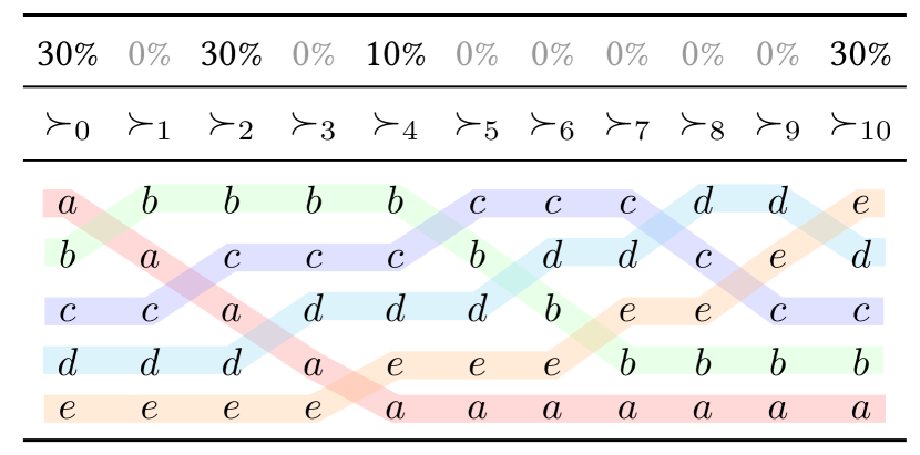
We say that a profile is single-crossing if the rankings in can be arranged in a single-crossing sequence. On single-crossing profiles, there is a natural definition of what it means to be an average, because each input ranking is associated with a location in a one-dimensional space; thus the output ranking should be at the weighted average of these locations. For example, the profile in Figure 5 has 30% of the voters each in locations 0, 2, and 10, with the remaining 10% in location 4. This gives an average location of . Thus, the “average” ranking for this profile is , and indeed this is the output ranking of Squared Kemeny. In contrast, the Kemeny rule takes the median location, which is location 2, and so is the Kemeny output.333This is known as the representative voter theorem (Rothstein, 1991) which states that the majority relation of a single-crossing profile (and hence the Kemeny ranking) coincides with the input ranking of the median voter.
To formalize this behavior, let us say that is compatible with a maximal single-crossing sequence if . We can now state an axiom specifying what it means to proportionally aggregate rankings on a single-crossing profile.
Single-Crossing-Proportionality.
An SPF satisfies Single-Crossing-Proportionality if for every single-crossing profile we have that a ranking is in if and only if there exists a maximal single-crossing sequence compatible with and for .
It is straightforward to check that Single-Crossing-Proportionality implies 2RP, because any profile in which only 2 rankings occur is single-crossing.
Theorem 3.1.
The Squared Kemeny rule satisfies Single-Crossing-Proportionality and 2RP.
Proof.
Since Single-Crossing-Proportionality implies 2RP, it is sufficient to prove that Squared Kemeny satisfies the former.
For this, we fix a single-crossing profile and an arbitrary maximal single-crossing sequence compatible with . Also, let be an arbitrary ranking and define . Because of the triangle inequality, we can now compute that
| (1) |
We will first show that if does not belong to any maximally single-crossing sequence compatible with , then at least one of Equation 1 for such that is strict. Assume otherwise, i.e., for every such that . If , this implies that , so belongs to the maximal single-crossing sequence . Thus, let us assume that . Then, let be maximal and minimal such that . By adding the respective equalities sidewise, we obtain that
By (Elkind et al., 2022, Proposition 4.6), this implies that , , and form a single-crossing sequence and is between and . This means that for every pair of alternatives such that , it holds that implies and implies . Consequently, the sequence is single-crossing, which contradicts the assumption that does not belong to any maximally single-crossing sequence compatible with .
Therefore, if does not belong to any maximally single-crossing sequence compatible with , we can show that there will be a ranking in such set, i.e., , for which . Indeed, from Equation 1 and the fact that one of them is strict, we get that
Thus, and we know that the only rankings selected by the Squared Kemeny rule belong to some maximally single-crossing sequence compatible with .
Then, take an arbitrary and again denote . This means that Taking the derivative with respect to , we get that is minimized when , which is equivalent to . Since has to be an integer and a quadratic function grows symmetrically from its minimum (note that a convex combination of quadratic functions is still a quadratic function), the rankings for have the lowest Squared Kemeny cost among the rankings in .
It remains to show that for selected in this way, the cost is the same no matter which maximally single-crossing sequence we have chosen at the beginning. To this end, take two arbitrary maximally single-crossing sequences and , both compatible with . Observe that there is a linear function , with such that for every . Then, by the linearity of the mean, if minimizes among , then minimizes among . Furthermore, we have that which concludes the proof. ∎
3.2. Characterization of the Squared Kemeny Rule
We will next present our characterization of the Squared Kemeny rule, which combines 2RP with three standard properties, namely neutrality, reinforcement, and continuity.
Neutrality.
Neutrality is a mild symmetry condition that precludes a rule from depending on the names of candidates. An SPF is neutral if for all profiles and permutations . Here, we denote by the ranking defined by if and only if for all and is the profile defined by for all .
Reinforcement.
Reinforcement is a classic axiom in social choice theory which describes that if some outcomes are chosen for two profiles, then precisely these common outcomes should be chosen in a convex combination of these profiles. An SPF satisfies reinforcement if for all profiles with , we have for all .
Continuity.
Continuity requires that a group of rankings with sufficient weight can overrule any other set of rankings and thus determine the outcome. Formally, an SPF is continuous if for all profiles , there is a scalar such that .
The above three axioms that have been frequently used in social choice theory to characterize scoring rules in various contexts (e.g., Young, 1975; Myerson, 1995; Skowron et al., 2019; Lackner and Skowron, 2021; Lederer, 2023). Moreover, Kemeny’s rule has been characterized as the unique SPF satisfying neutrality, reinforcement, and a Condorcet axiom (Young and Levenglick, 1978).
We can now state our characterization result.
Theorem 3.2.
An SPF satisfies neutrality, reinforcement, continuity, and 2RP if and only if it is the Squared Kemeny rule.
Like other reinforcement-based characterizations of SPFs, our proof is quite involved, and thus we defer it to Appendix A. Using well-known techniques, the proof uses reinforcement to divide the space of profiles into convex regions where a particular ranking is chosen by the SPF, and then uses 2RP in combination with the other axioms to characterize the boundaries (hyperplanes) of these regions. As for the independence of the axioms, we do not know if neutrality or continuity can be dropped from the characterization. Without 2RP, the Kemeny rule satisfies the remaining axioms. Without reinforcement, the rule that agrees with the Squared Kemeny rule on all profiles in which two rankings jointly have more than 90% of the weight, and returns the set of all rankings for all other profiles, satisfies the remaining axioms.
To give more insights into the proof of Theorem 3.2, we will show a weaker statement that is still of interest. To this end, we introduce the family of ranking scoring functions. These are analogues of scoring rules in voting and are defined based on a cost function that assigns to each pair of rankings a cost . Intuitively, we interpret the term as the disutility that the outcome ranking would give to a voter with a preference order . The ranking scoring function based on returns the rankings with minimal total cost: for every profile . For example, is the Kemeny rule and is the Squared Kemeny rule.
It is straightforward to check that every ranking scoring function satisfies reinforcement and continuity. The class of (neutral) ranking scoring functions was introduced by Conitzer et al. (2009), who conjectured that this class is in fact characterized by neutrality, reinforcement, and continuity.
We now give a proof that the only ranking scoring function that satisfies the 2RP axiom is the Squared Kemeny rule. The proof uses a very similar strategy to the proof of our full axiomatic characterization (Theorem 3.2) but avoids some of its overhead. Note that this version of the characterization does not require neutrality.
Theorem 3.3.
A ranking scoring function satisfies 2RP if and only if it is the Squared Kemeny rule.
Proof.
We already showed that the Squared Kemeny rule satisfies 2RP (Theorem 3.1), so we need to show that it is the only ranking scoring function with that property. Hence, let denote a ranking scoring function that satisfies 2RP and let be its cost function. Without loss of generality, we can assume for every ranking that because adding a constant to a cost function, even a different constant for each first argument, does not affect the outcomes of a ranking scoring function. For a profile and a ranking , we define . We will show that is proportional to the Squared Kemeny cost function , which implies that is the Squared Kemeny rule. We prove this in three steps: first, we will show that for every pair of rankings with swap distance , the difference in the costs of and with respect to any other ranking is proportional to the difference in their Squared Kemeny costs, i.e., there exists a constant such that for every (Step 1). Next, we will prove that these constants are equal if two such pairs of rankings intersect, i.e., for all such that (Step 2). Finally, we infer that all these constants are equal and derive that there is such that for all . Since for all , this means that is indeed proportional to (Step 3).
Step 1: Fix two rankings with and define . We will show that and for all . Let us first prove that is equal to . For this, we consider the profile with . 2RP requires that . Thus, from the definition of ranking scoring functions and our assumption that for every we derive that and therefore
| (2) |
To show that , consider another profile with and . By 2RP, we get that and thus that . Because and , we derive that .
Now, fix an arbitrary ranking . Since , there is exactly one pair of alternatives on which and disagree. Let us denote them by and , i.e., and . We subsequently assume that and discuss the case that later. Let and observe that (see Figure 6 for an illustration). Moreover, we define as the profile with and . Since and , 2RP implies that . Thus, by the definition of ranking scoring functions, , which further implies that . We can now compute that
Since , it follows that .
Lastly, let us consider the case of . By analogous reasoning, we obtain that . By Equation 2 and sidewise multiplication by , we hence infer the thesis of this Step also in this case.
Step 2: Consider three rankings with and let and denote the constants derived in the previous step. We will show in this step that . If , then necessarily and our claim directly follows from Equation 2.
Thus, assume , let denote the ranking that is completely reverse of , and let . Furthermore, we define as the profile with and (see Figure 6 for an illustration). Observe that and . Hence, 2RP implies that all rankings in swap distance from are selected by . In particular, . By the definition of the ranking scoring function, this means that , and therefore also . Next, Step 1 implies that and . Since we have , we now derive that
Hence, by Equation 2, it follows that .
Step 3: Finally, we will show that is proportional to , so that is the Squared Kemeny rule. To this end, we first show that , for all with . To see this, observe that there exists a sequence of rankings such that , , , , and for every . Then, Step 2 implies that . We hence drop the index of these constants and simply refer to them by .
Next, take arbitrary rankings and let be a sequence of rankings such that , , and for every . Using the “telescoping sum” technique twice, we get that
From this we get that is proportional to . Indeed, for every two rankings , we get that Since , this means that is the Squared Kemeny rule. ∎
3.3. Efficiency, Participation, and Strategyproofness
We will next show that the Squared Kemeny rule satisfies desirable efficiency and participation properties but violates strategyproofness. To define these axioms for SPFs, we first need to specify how we compare two output rankings , based on an input ranking . Following the literature (e.g., Bossert and Storcken, 1992; Bossert and Sprumont, 2014; Athanasoglou, 2016), we use the swap distance between the input ranking and the output rankings: given an input ranking , is weakly preferred to (denoted by ) if , and is strictly preferred to (denoted by ) if . It does not make a difference for these purposes whether we use the swap distance or the squared swap distance since they induce the same preferences. Next, we will define efficiency, participation, and strategyproofness.
Efficiency.
An outcome is (Pareto) efficient if it is not possible to make one voter better off without making any other voter worse off. Formally, we say that a ranking dominates another ranking in a profile if for all and for some . Moreover, a ranking is efficient for a profile if it is not dominated by any other ranking. Finally, an SPF is efficient if, for every profile , every ranking is efficient.444Bossert and Sprumont (2014) show that if for all , then we also have whenever is efficient in .
Participation.
The axiom of participation is typically formulated in electoral settings and intuitively requires that it is never better for a group of agents to abstain from an election than to participate. In our context, participation can be seen as a consistency notion: if is a winning ranking in the profile and we add additional criteria to according to which is better than , then should not be winning in the extended profile. More formally, we say an SPF satisfies participation if there are no profiles , a constant , and rankings , such that for all and for some .
Strategyproofness.
As the last axiom of this section, we will consider strategyproofness. This axiom is also typically studied in electoral settings and requires that agents should never be better off by lying than by voting truthfully. We hence say an SPF is strategyproof if there are no profiles , , rankings , , and a constant such that (i) and for some rankings with , and (ii) , , and for all .
Proposition 3.4.
The Squared Kemeny rule satisfies efficiency and participation but violates strategyproofness.
Proof.
We first show that Squared Kemeny is efficient. For this, let be a profile and , be two rankings such that dominates in . It is easy to check that , so , which implies that the Squared Kemeny rule is indeed efficient.
For participation, consider two profiles , , and two rankings , such that , for all , and for some . Since , we have . Moreover, from the conditions on we get that . This implies for every that because
Hence, the Squared Kemeny rule indeed satisfies participation.
Finally, we turn to strategyproofness, and consider the following two profiles and .
|
:
|
:
|
It can be verified that Squared Kemeny uniquely chooses the ranking for and the ranking for . Since the profile arises from the profile by moving probability from to and , this shows that the Squared Kemeny rule is manipulable. This example also shows that Squared Kemeny fails the weaker “betweenness” version of strategyproofness of Bossert and Sprumont (2014), which Kemeny does satisfy. ∎
4. Proportionality Guarantees
In our axiomatic treatment, we have discussed the behavior of the Squared Kemeny rule on profiles with a lot of structure (single-crossing) and in particular those with only two rankings (2RP). Does Squared Kemeny retain its behavior as an average in general? This is what we will quantify in this section. As an initial matter, we can check what Squared Kemeny does on profiles in which three rankings occur. For a fixed set of three rankings, we can use a simplex of weights to picture all profiles based on these rankings. For each point of the simplex (i.e., for each profile), we can compute the Kemeny and Squared Kemeny outcomes, and we can color the point to indicate how close the output rankings are to each of the input rankings. We show the result of this exercise in Figure 7. This confirms our expectation that Squared Kemeny takes rankings with smaller weight into account, while Kemeny frequently ignores them.
For general profiles with any number of rankings, we can ask about the maximum (over all possible profiles) swap distance between the output ranking and an input ranking, as a function of its weight . For an ideal proportional rule, there should be a roughly linear relationship between these. For Kemeny, the distance can be as large as (the maximum possible swap distance) when , and it is when . For Squared Kemeny, we can compute its behavior for fixed using a linear program (see Section B.1) that searches for the worst-case profile, which yields the plot in Figure 3 shown in the introduction. That function is approximately linear, except for a “hump” for small , which indicates that Squared Kemeny can output the reverse of an input ranking which has weight as large as . We do not have a satisfactory explanation for these humps (the profiles witnessing this worst-case behavior are very complicated, see Section B.2), and we do not know how big the hump is as , but we do know it cannot exceed (by Theorem 4.2 below). In addition to computing the exact worst-case behavior for fixed , we can also prove a theoretical upper bound that works for any , which bounds the distance between the Squared Kemeny ranking and a weight- input ranking. This bound is also shown in Figure 3.
Theorem 4.1.
Let be a profile and let be a ranking with weight . Then
Proof.
Note that since is the maximum swap distance between two rankings, and an fraction of the profile has swap distance to . Let be a ranking selected by Squared Kemeny and write . Then we have . Because optimizes the Squared Kemeny cost, we have and thus . Solving for , we get , as required. ∎
The above bound makes sense for profiles with few rankings that are not very similar to each other. But in contexts with many rankings, some of which are similar to each other, it would be better to guarantee to groups of rankings that the output ranking should not be too far away from them, on average. We will formalize this in a similar way to the work of Skowron and Górecki (2022), by considering arbitrary groups of rankings, without making any cohesiveness assumptions (that would say that the rankings in a group must be similar to each other). Note that such a setup limits the guarantees we can give: for a group of size (i.e. all the rankings together), we cannot guarantee that the output agrees with the group on more than half the pairwise comparisons on average (consider for example a profile where one ranking and its reverse each have weight ).
To state our result, given a profile , we say that is a subprofile of if for all rankings . The size of is . We can think of as a group of voters, and its size as the fraction of the entire electorate that they make up. We now provide a bound on the average satisfaction of any group.
Theorem 4.2.
Let be a profile and let be a subprofile of with size . Then
Proof.
Let be the maximum swap distance between two rankings. Fix any ranking . For each , let be the number of rankings with . The values are the Mahonian numbers and it is known (Ben-Naim, 2010) that
For a fixed profile , the average Squared Kemeny cost over all rankings is
Therefore, there exists a ranking such that . From minimality of Squared Kemeny, we know that this is true for any . Since is a subprofile of ,
Finally, by Jensen’s inequality we get that since the square function is convex, which yields the thesis.∎
In Figure 8, we show the upper bound obtained in Theorem 4.2 in terms of normalized swap distance (so is mapped to 1). For , we also show the actual worst-case performance of Squared Kemeny, which can be computed for fixed using linear programs for finding worst-case profiles that maximize the distance between the output and some size- group. The figure also shows a lower bound, which is obtained by linear programs that find profiles where all output rankings are bad simultaneously in the sense that some size- group incurs at least the lower bound’s distance.
5. Computation
The computational complexity of the Kemeny rule has been extensively studied. The problem of deciding if there is a ranking with at most a given cost is NP-complete (Bartholdi, III et al., 1989), even for a constant number of input rankings (Dwork et al., 2001; Biedl et al., 2009; Bachmeier et al., 2019). Thus, it is reasonable to expect that the analogous problem for the Squared Kemeny rule is also NP-complete, and this is indeed the case, see Section C.1.
Theorem 5.1.
The problem of deciding, given a profile and a number , whether there exists a ranking with , is NP-complete, even for profiles with 4 rankings with equal weight.
The proof is by reduction from the problem for the Kemeny rule, and uses the same technique used by Biedl et al. (2009) for showing that the egalitarian Kemeny rule (which selects the ranking where the maximum swap distance to any input ranking is minimized) is NP-complete to compute.
There exists an ILP formulation for computing the Kemeny rule, which is reasonably efficient in practice (Conitzer et al., 2006). While this ILP formulation depends on the linear nature of the Kemeny objective, it is still possible to give an ILP formulation for the Squared Kemeny rule, using the same trick used by Caragiannis et al. (2019) for computing the maximum Nash welfare solution for fair allocation, and generalized by Bredereck et al. (2020) for various covering problems. The encoding is described in Section C.2. We found that it allows us to evaluate the Squared Kemeny rule reasonably efficiently up to (see Figure 9).555We note that outliers (with up to times longer running time than the median) do occur.
The Kemeny rule also admits efficient approximation algorithms (Ailon et al., 2008; Van Zuylen and Williamson, 2009; Coppersmith et al., 2010) and even a PTAS (Kenyon-Mathieu and Schudy, 2007). The Squared Kemeny rule admits a simple 4-approximation algorithm (output the input ranking that has the best score, see Section C.3). In addition, we can show that the optimal Kemeny ranking provides a 2-approximation to the Squared Kemeny rule. Combining this with the known PTAS for Kemeny, we obtain the following result, proved in Section C.4:
Theorem 5.2.
For every constant , there exists a polynomial-time -approximation to the Squared Kemeny rule.
We believe, however, that such approximation algorithms have limited interest for our applications, since a ranking may have a good approximation factor to the optimum Squared Kemeny score while not satisfying the desirable proportionality properties of the Squared Kemeny rule. Indeed, the rankings returned by Kemeny and Squared Kemeny may be very far apart from each other (in the extreme case, they may be opposite to each other except for 1 shared pairwise comparison, see Section C.5), even though Kemeny provides a 2-approximation to Squared Kemeny. Still, approximation algorithms may have their use, for example, as subroutines in branch and bound algorithms. We leave the question of whether Squared Kemeny admits a PTAS to future work.
6. Empirical Analysis
In this section, we compare the performance of the Squared Kemeny rule and the Kemeny rule based on several empirical experiments.
| Rank | GDP pc. (40%) | Air Quality (30%) | Sunniness (30%) | Kemeny | Sq. Kemeny | |
| 1. | San Francisco | New York City | San Francisco | San Francisco | () | |
| 2. | New York City | Cairo | New York City | New York City | () | |
| 3. | Johannesburg | Sydney | () | |||
| 4. | Buenos Aires | San Francisco | () | |||
| 5. | Sydney | London | Lahore | Sydney | () | |
| 6. | Sydney | Rome | Rome | () | ||
| 7. | London | Rio de Janeiro | Sydney | London | Johannesburg | () |
| 8. | Paris | San Francisco | Mumbai | Tokyo | Buenos Aires | () |
| 9. | Hong Kong | New York City | Paris | Rio de Janeiro | () | |
| 10. | Tokyo | Tokyo | Mexico | Hong Kong | () | |
| 11. | Rome | Buenos Aires | () | |||
| 12. | Rome | Moscow | Bangkok | Rome | London | () |
| 13. | Seoul | Paris | Rio de Janeiro | Johannesburg | Tokyo | () |
| 14. | Moscow | Hong Kong | Istanbul | Buenos Aires | Hong Kong | () |
| 15. | Shanghai | Mexico | Seoul | Rio de Janeiro | Mexico | () |
| 16. | Johannesburg | Johannesburg | Seoul | Seoul | () | |
| 17. | Rio de Janeiro | Seoul | Tokyo | Moscow | Moscow | () |
| 18. | Istanbul | Bangkok | Shanghai | Mexico | Paris | () |
| 19. | Buenos Aires | Istanbul | Lagos | Bangkok | Bangkok | () |
| 20. | Mexico | Lagos | Hong Kong | Istanbul | Istanbul | () |
| 21. | Bangkok | Shanghai | Moscow | Shanghai | Shanghai | () |
| 22. | Mumbai | Cairo | Paris | Cairo | Cairo | () |
| 23. | Cairo | Mumbai | Mumbai | () | ||
| 24. | Lagos | Mumbai | London | Lagos | Lagos | () |
| 25. | Lahore | Lahore | Lahore | Lahore | () |
6.1. Aggregate City Ranking
Our first experiment is a detailed example. We selected cities around the world and ranked them, based on their Gross Domestic Product (GDP) per capita, air quality (measured by average PM 2.5 concentration), and sunniness (based on the average number of sunshine hours in a year). The details of the sources used can be found in Section D.1. Then, we assigned weight to GDP per capita, to air quality, and to sunniness. We aggregated the rankings using the Kemeny and Squared Kemeny rules. While Squared Kemeny selected a unique ranking, Kemeny selected tied outputs, in which a few cities differ by to positions. When increasing the weight on the GDP ranking by a small amount, only one of these outputs stays optimal, and we went with that output. The aggregation results are presented in Table 1.
Note that the top- of the Kemeny ranking is identical to the top- of the GDP per capita ranking. This includes Dublin and Zurich, which are both in the bottom- of the sunniness ranking. This is exactly the behavior we would like to avoid in the proportional aggregation of rankings: focusing mainly on one input ranking and disregarding another with still significant weight assigned to it.
In contrast, both Dublin and Zurich do not appear in the top- of the ranking selected by the Squared Kemeny rule. Instead, its top- includes Toronto (which is in the middle of the sunniness ranking and relatively high in both GDP per capita and air quality rankings) and Dubai (which, although near the bottom of the air quality ranking, is the first according to sunniness and -th based on GDP per capita). In this way, the top- of the Squared Kemeny rule output ranking arguably offers more uniform representation of the highest ranked cities across all input rankings.
6.2. Drawing Embeddings of Rankings
Next, we visualize how the rankings output by the Kemeny and Squared Kemeny rules relate to the input rankings, using two methods of embedding rankings into 2-dimensional Euclidean space.
The first method is called map of preferences, introduced by Faliszewski et al. (2023), and starts by computing the swap distances between each pair of rankings present in a profile. Then, we apply a classical multidimensional scaling algorithm (Torgerson, 1952) to put each ranking as a dot on a plane in such a way that the Euclidean distances between the dots reflect the swap distances between the rankings as well as possible. By the size of a dot we signify the weight of a given ranking in the profile. In order to obtain the coordinates for the outputs of the Kemeny and Squared Kemeny rules as well, we simply include them while computing the distance matrix.
Figure 10 presents maps of preferences of six profiles which we have generated using different models. For each, we sampled 200 rankings, with possible repetitions, over 10 alternatives and constructed the profile by assigning each ranking a weight proportional to the number of times it was sampled. We have also verified that the behavior of Kemeny and Squared Kemeny visible on these examples is consistent across different profiles generated in the same way.
The first two pictures present profiles drawn from the Euclidean model, in which we sample 10 alternative points and 200 voter points uniformly at random from the unit disc (the first picture) or from its boundary, the unit circle (second picture). Then, for every voter point we record a ranking of all alternatives in order of increasing distance from the voter. For the disc, the Kemeny and Squared Kemeny rules select rankings very close to each other. However, for the circle, the difference is significant. While Squared Kemeny chooses a ranking that is in the center, Kemeny outputs a ranking that is similar to one of the input rankings on a circle. This is because for every ranking on the circle, we also have the reversed (or close to the reversed) ranking on the opposite side of the circle. Thus, all possible rankings have a similar average swap distance to the profile and the smallest occurs on the part of the circle from which, by chance, we sampled more voter points, which is then chosen by Kemeny. In contrast, since Squared Kemeny minimizes the average squared swap distance, it tries to equalize the distances to all rankings present in the profile.
The next two pictures show the maps of preferences for profiles generated from the mixture of two Mallows models (Mallows, 1957). Given a central ranking and a noise parameter , we sample each ranking with probability proportional to under the Mallows model. Thus, for smaller , the distribution is more concentrated around . We generated of the rankings using one Mallows model with the central ranking and noise and using another Mallows model with the central ranking that is the complete reverse of and noise . When (the third picture), the Kemeny rule outputs , the central ranking of the Mallows model responsible for of the rankings while the Squared Kemeny rule selects a ranking in between and . Interestingly, if is significantly smaller than (the fourth picture), the Kemeny rule outputs the central ranking of the smaller but more concentrated model, while Squared Kemeny is still between and . This confirms our intuition that Squared Kemeny works like an average of rankings.
Finally, the last two pictures present the profiles drawn from models based on real-world data from Preflib (Mattei and Walsh, 2013): the breakfast dataset (Green and Rao, 1972) that contains 42 preference orders over 15 breakfast items; and the 2016 countries ranking dataset (Boehmer and Schaar, 2023), where 107 countries are ranked according to 14 different criteria. For each dataset, we sampled with replacement 200 rankings and then restricted each ranking to 10 randomly chosen alternatives. For both profiles, Kemeny and Squared Kemeny choose similar rankings, with the former closer to the most concentrated part, and the latter closer to the center of the picture.
The second method of visualizing the positions of rankings is specific to profiles drawn from the Euclidean model. Given a profile specified by voter and alternative locations, and given an output ranking , we try to find a point in the same Euclidean space that would induce the ranking . In general, such a point may not exist, but using an ILP we can find a point that induces a ranking with minimal possible swap distance to .
In our experiments shown in Figure 11, we sample candidate locations uniformly from the unit square, and voter locations according to different distributions of interest. We then compute the outputs of the Kemeny and Squared Kemeny rules and embed them as a point in space. For each voter location distribution, we repeat this process 100 times and superimpose the results for the 100 profiles in the same figure, showing voters as blue dots, Kemeny rankings as red diamonds, and Squared Kemeny rankings as green squares.
The first voter distribution samples the voter locations uniformly from the unit disc, and we see that both rules select central rankings, with somewhat more variance in the Kemeny rankings. For the second and third picture, we sample voter locations from two Gaussians centered in the bottom left and top right corners. In the second picture, we sample 20 voters each from the two Gaussians and see that both rules select rankings roughly midway between the center points of the Gaussians. In the third picture, we sample 30 voters from the bottom left and 10 voters from the top right. Kemeny selects rankings located within the bigger cluster, while Squared Kemeny chooses locations that interpolate between the two (while still being closer to the larger cluster). The fourth and fifth picture repeat the same process with four Gaussians with voters uniformly distributed (in the fourth picture) or with 25 voters in the bottom left and 5 voters each in the other three clusters.
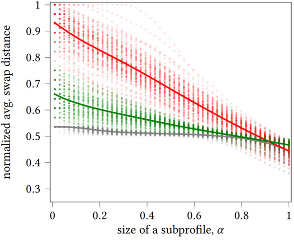
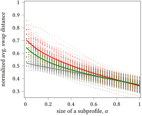
6.3. Worst-Case Average Distance
Our final experiment revisits the problem studied in Section 4, where we considered the average distance between the rankings of a group of voters and the output ranking. There, we bounded the distance for the worst-case profile, while here we compute it for randomly sampled profiles. Consider a profile and an output ranking . For each size , we look for the “unhappiest” group (i.e., subprofile of ) of size , in the sense that the average distance between and the rankings of is large. Formally, we define for this worst average distance, where denote that is a subprofile of with size .
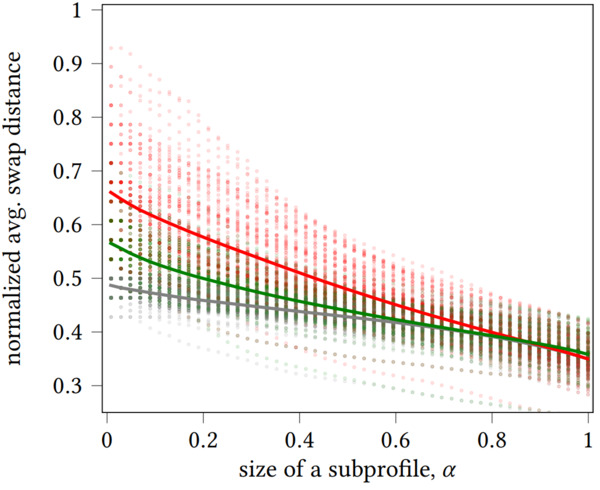
For the experiment, we sampled 100 profiles with 8 alternatives and 50 rankings according to various distributions. The results of our experiment for the Euclidean disc model is presented in Figure 12. (See Section D.2 for other distributions.) For each profile and each size , we put a red dot indicating the value of for Kemeny, and a green dot for Squared Kemeny. The lines show the average value for each .
Figure 12 also shows a lower bound. For each , this is computed by finding the ranking that optimizes , and placing a gray dot at that value. Note that different rankings may be optimum for different , and so this lower bound is “unfair” to rules like Kemeny or Squared Kemeny, which must choose a single ranking which gets evaluated for all simultaneously.
We see that when is close to , Kemeny leads to smaller distances than Squared Kemeny. This is to be expected, as Kemeny minimizes the overall average distance. However, for smaller than , it is Squared Kemeny that returns the lower values on average. Observe also that the difference between the Kemeny and Squared Kemeny for close to is negligible, while the differences for close to are significant or even substantial depending on the considered model.
7. Conclusions and Future Work
We have studied the Squared Kemeny rule and argued that it behaves more appropriately in contexts where we want to aggregate rankings proportionally, compared to its better-known cousin the Kemeny rule. In particular, we have shown a full characterization of the Squared Kemeny rule based on a proportionality axiom, proved general proportionality guarantees for this rule, and demonstrated in an experimental study that it behaves similar to a mean. Based on these results, we conclude that the Squared Kemeny rule has the potential of providing a consensus ranking in situations where a majoritarian rule such as Kemeny is undesirable.
There are many interesting directions for future work exploring the topic of proportional rank aggregation. In particular, one could study new SPFs with the aim to find more proportional rules. For instance, one could consider rules based on the Spearman footrule distance instead of the swap distance (Diaconis and Graham, 1977; Viappiani, 2015), analogues of Proportional Approval Voting (Aziz et al., 2017), or the family of “-Kemeny rules” that minimize the -th power of the swap distance. One could also derive other proportionality axioms that are not defined in terms of swap distance. For example, following Skowron et al. (2017) who study proportional rankings based on approval votes, one could phrase proportionality as requiring that every top-initial segment of the output ranking, viewed as a set, should be a proportional committee. How to adapt this to ranking input is not clear, though, since it is an open question whether axioms for proportional multi-winner rules (such as Proportionality for Solid Coalitions, PSC, Aziz and Lee, 2020) are compatible with committee monotonicity, which is necessary to adapt a multi-winner rule to output a ranking.
Finally, we note that the methods that we have introduced may prove useful in other contexts. For example, we considered bounds on the maximum dissatisfaction of a voter, as a function of the voter’s weight. Plotting and bounding these functions could provide insights in all kinds of collective decision-making problems. Further, our work can be seen as proportional decision-making on binary issues (“should be ranked above ?”) under constraints (in our case, transitivity). This general topic has just started to be explored by researchers (Skowron and Górecki, 2022; Lackner and Maly, 2023; Chandak et al., 2024; Masařík et al., 2023).
Acknowledgements
This work was funded in part by the French government under management of Agence Nationale de la Recherche as part of the “Investissements d’avenir” program, reference ANR-19-P3IA-0001 (PRAIRIE 3IA Institute).
References
- (1)
- Ailon et al. (2008) Nir Ailon, Moses Charikar, and Alantha Newman. 2008. Aggregating inconsistent information: ranking and clustering. Journal of the ACM (JACM) 55, 5 (2008), 1–27. https://doi.org/10.1007/BF01200760
- Athanasoglou (2016) Stergios Athanasoglou. 2016. Strategyproof and efficient preference aggregation with Kemeny-based criteria. Games and Economic Behavior 95 (2016), 156–167. https://doi.org/10.1016/j.geb.2015.12.002
- Aziz et al. (2017) Haris Aziz, Markus Brill, Vincent Conitzer, Edith Elkind, Rupert Freeman, and Toby Walsh. 2017. Justified representation in approval-based committee voting. Social Choice and Welfare 48, 2 (2017), 461–485. https://doi.org/10.1007/s00355-016-1019-3
- Aziz and Lee (2020) Haris Aziz and Barton E. Lee. 2020. The expanding approvals rule: improving proportional representation and monotonicity. Social Choice and Welfare 54 (2020), 1–45. https://doi.org/10.1007/s00355-019-01208-3
- Bachmeier et al. (2019) Georg Bachmeier, Felix Brandt, Christian Geist, Paul Harrenstein, Keyvan Kardel, Dominik Peters, and Hans Georg Seedig. 2019. -Majority digraphs and the hardness of voting with a constant number of voters. J. Comput. System Sci. 105 (2019), 130–157. https://doi.org/10.1016/j.jcss.2019.04.005
- Bartholdi, III et al. (1989) John Bartholdi, III, Craig A. Tovey, and Michael A. Trick. 1989. Voting schemes for which it can be difficult to tell who won the election. Social Choice and Welfare 6 (1989), 157–165. https://doi.org/10.1007/BF00303169
- Ben-Naim (2010) Eli Ben-Naim. 2010. Mixing of diffusing particles. Physical Review E 82, 6 (2010), 061103. https://doi.org/10.1103/PhysRevLett.102.190602
- Biedl et al. (2009) Therese Biedl, Franz J. Brandenburg, and Xiaotie Deng. 2009. On the complexity of crossings in permutations. Discrete Mathematics 309, 7 (2009), 1813–1823. https://doi.org/10.1016/j.disc.2007.12.088
- Boehmer and Schaar (2023) Niclas Boehmer and Nathan Schaar. 2023. Collecting, classifying, analyzing, and using real-world elections. In Proceedings of the 22nd International Conference on Autonomous Agents and Multiagent Systems (AAMAS). 1706–1715. https://www.ifaamas.org/Proceedings/aamas2023/pdfs/p1706.pdf
- Bossert and Sprumont (2014) Walter Bossert and Yves Sprumont. 2014. Strategy-proof preference aggregation: Possibilities and characterizations. Games and Economic Behavior 85 (2014), 109–126. https://doi.org/10.1016/j.geb.2014.01.015
- Bossert and Storcken (1992) Walter Bossert and Ton Storcken. 1992. Strategy-proofness of social welfare functions: The use of the Kemeny distance between preference orderings. Social Choice and Welfare 9 (1992), 345–360. https://doi.org/10.1007/BF00182575
- Bredereck et al. (2020) Robert Bredereck, Piotr Faliszewski, Rolf Niedermeier, Piotr Skowron, and Nimrod Talmon. 2020. Mixed integer programming with convex/concave constraints: Fixed-parameter tractability and applications to multicovering and voting. Theoretical Computer Science 814 (2020), 86–105. https://doi.org/10.1016/j.tcs.2020.01.017
- Caragiannis et al. (2019) Ioannis Caragiannis, David Kurokawa, Hervé Moulin, Ariel D. Procaccia, Nisarg Shah, and Junxing Wang. 2019. The unreasonable fairness of maximum Nash welfare. ACM Transactions on Economics and Computation (TEAC) 7, 3 (2019), 1–32. https://doi.org/10.1002/cpa.3160130102
- Chakraborty et al. (2022) Diptarka Chakraborty, Syamantak Das, Arindam Khan, and Aditya Subramanian. 2022. Fair rank aggregation. Advances in Neural Information Processing Systems (NeurIPS) 35 (2022), 23965–23978. https://proceedings.neurips.cc/paper_files/paper/2022/file/974309ef51ebd89034adc64a57e304f2-Paper-Conference.pdf
- Chandak et al. (2024) Nikhil Chandak, Shashwat Goel, and Dominik Peters. 2024. Proportional aggregation of preferences for sequential decision making. In Proceedings of the 38th AAAI Conference on Artificial Intelligence (AAAI). https://arxiv.org/abs/2306.14858
- Conitzer et al. (2006) Vincent Conitzer, Andrew Davenport, and Jayant Kalagnanam. 2006. Improved bounds for computing Kemeny rankings. In Proceedings of the 21st National Conference on Artificial Intelligence (AAAI). 620–626. https://www.cs.cmu.edu/~conitzer/kemenyAAAI06.pdf
- Conitzer et al. (2009) Vincent Conitzer, Matthew Rognlie, and Lirong Xia. 2009. Preference functions that score rankings and maximum likelihood estimation. In Proceedings of the 21st International Joint Conference on Artificial Intelligence (IJCAI). 109–115. http://www.cs.cmu.edu/~conitzer/preferenceIJCAI09.pdf
- Coppersmith et al. (2010) Don Coppersmith, Lisa K. Fleischer, and Atri Rurda. 2010. Ordering by weighted number of wins gives a good ranking for weighted tournaments. ACM Transactions on Algorithms (TALG) 6, 3 (2010), 1–13. https://doi.org/10.1007/BF01200760
- Diaconis and Graham (1977) Persi Diaconis and Ronald L. Graham. 1977. Spearman’s footrule as a measure of disarray. Journal of the Royal Statistical Society Series B: Statistical Methodology 39, 2 (1977), 262–268. https://doi.org/10.1111/j.2517-6161.1977.tb01624.x
- Dwork et al. (2001) Cynthia Dwork, Ravi Kumar, Moni Naor, and Dandapani Sivakumar. 2001. Rank aggregation methods for the web. In Proceedings of the 10th International Conference on World Wide Web (WWW). 613–622. https://doi.org/10.1145/371920.372165
- Elkind et al. (2022) Edith Elkind, Martin Lackner, and Dominik Peters. 2022. Preference restrictions in computational social choice: A survey. arXiv:2205.09092 [cs.GT]
- Faliszewski et al. (2023) Piotr Faliszewski, Andrzej Kaczmarczyk, Krzysztof Sornat, Stanisław Szufa, and Tomasz W\kas. 2023. Diversity, agreement, and polarization in elections. In Proceedings of the 32nd International Joint Conference on Artificial Intelligence (IJCAI). 2684–2692. https://doi.org/10.24963/ijcai.2023/299
- Fishburn (1978) Peter C. Fishburn. 1978. Axioms for approval voting: Direct proof. Journal of Economic Theory 19, 1 (1978), 180–185. https://doi.org/10.1016/0022-0531(78)90062-5
- Green and Rao (1972) Paul E. Green and Vithala R. Rao. 1972. Applied multidimensional scaling: A comparison of approaches and algorithms.
- Kemeny (1959) John G. Kemeny. 1959. Mathematics without numbers. Daedalus 88, 4 (1959), 577–591. https://www.jstor.org/stable/20026529
- Kemeny and Snell (1960) John G. Kemeny and J. Laurie Snell. 1960. Preference rankings: An axiomatic approach. In Mathematical Models in the Social Sciences. Ginn, 9–23.
- Kenyon-Mathieu and Schudy (2007) Claire Kenyon-Mathieu and Warren Schudy. 2007. How to rank with few errors: A PTAS for weighted feedback arc set on tournaments. In Proceedings of the 39th Annual ACM Symposium on Theory of Computing (STOC). 95–103. https://doi.org/10.1145/1250790.1250806
- Kuhlman and Rundensteiner (2020) Caitlin Kuhlman and Elke Rundensteiner. 2020. Rank aggregation algorithms for fair consensus. Proceedings of the VLDB Endowment 13 (2020), 2706–2719. https://doi.org/10.14778/3407790.3407855
- Lackner and Maly (2023) Martin Lackner and Jan Maly. 2023. Proportional decisions in perpetual voting. In Proceedings of the 37th AAAI Conference on Artificial Intelligence (AAAI). 5722–5729. https://doi.org/10.1609/aaai.v37i5.25710
- Lackner and Skowron (2021) Martin Lackner and Piotr Skowron. 2021. Consistent approval-based multi-winner rules. Journal of Economic Theory 192 (2021), 105173. https://doi.org/10.1016/j.jet.2020.105173
- Lackner and Skowron (2023) Martin Lackner and Piotr Skowron. 2023. Multi-Winner Voting with Approval Preferences. Springer. https://doi.org/10.1007/978-3-031-09016-5
- Lederer (2023) Patrick Lederer. 2023. Bivariate scoring rules: Unifying the characterizations of positional scoring rules and Kemeny’s rule. (2023). https://pub.dss.in.tum.de/brandt-research/consistent_ranking.pdf
- Mallows (1957) Colin L. Mallows. 1957. Non-null ranking models. Biometrika 44 (1957), 114–130. https://doi.org/10.2307/2333244
- Masařík et al. (2023) Tomáš Masařík, Grzegorz Pierczyński, and Piotr Skowron. 2023. A generalised theory of proportionality in collective decision making. arXiv:2307.06077 [cs.GT]
- Mattei and Walsh (2013) Nicholas Mattei and Toby Walsh. 2013. Preflib: A library for preferences. In Proceedings of the 4rd International Conference on Algorithmic Decision Theory (ADT). Springer, 259–270. https://doi.org/10.1111/j.1467-9280.2007.01950.x
- Myerson (1995) Roger B. Myerson. 1995. Axiomatic derivation of scoring rules without the ordering assumption. Social Choice and Welfare 12, 1 (1995), 59–74. https://doi.org/10.1007/BF00182193
- Oğuz (2023) Selin Oğuz. 2023. Mapped: Air pollution levels around the world in 2022. VC Elements (2023). https://elements.visualcapitalist.com/mapped-air-pollution-levels-around-the-world-2022/
- Peters et al. (2021) Dominik Peters, Grzegorz Pierczyński, and Piotr Skowron. 2021. Proportional participatory budgeting with additive utilities. Advances in Neural Information Processing Systems 34 (2021), 12726–12737. https://arxiv.org/abs/2008.13276
- Rothstein (1991) Paul Rothstein. 1991. Representative voter theorems. Public Choice 72, 2-3 (1991), 193–212. https://doi.org/10.1007/BF00123744
- Skowron et al. (2019) Piotr Skowron, Piotr Faliszewski, and Arkadii Slinko. 2019. Axiomatic characterization of committee scoring rules. Journal of Economic Theory 180 (2019), 244–273. https://doi.org/10.1016/j.jet.2018.12.011
- Skowron and Górecki (2022) Piotr Skowron and Adrian Górecki. 2022. Proportional public decisions. In Proceedings of the 36th AAAI Conference on Artificial Intelligence (AAAI). 5191–5198. https://doi.org/10.1609/aaai.v36i5.20454
- Skowron et al. (2017) Piotr Skowron, Martin Lackner, Markus Brill, Dominik Peters, and Edith Elkind. 2017. Proportional rankings. In Proceedings of the 26th International Joint Conference on Artificial Intelligence. 409–415. https://www.ijcai.org/Proceedings/2017/0058.pdf
- Torgerson (1952) Warren S. Torgerson. 1952. Multidimensional scaling: I. Theory and method. Psychometrika 17, 4 (1952), 401–419. https://doi.org/10.1007/BF02288916
- Van Zuylen and Williamson (2009) Anke Van Zuylen and David P. Williamson. 2009. Deterministic pivoting algorithms for constrained ranking and clustering problems. Mathematics of Operations Research 34, 3 (2009), 594–620. https://doi.org/10.1007/978-3-540-77918-6_21
- Viappiani (2015) Paolo Viappiani. 2015. Characterization of scoring rules with distances: application to the clustering of rankings. In Proceedings of the 24th International Joint Conference on Artificial Intelligence (IJCAI). 104–110. http://ijcai.org/papers15/Papers/IJCAI15-022.pdf
- Wei et al. (2022) Dong Wei, Md Mouinul Islam, Baruch Schieber, and Senjuti Basu Roy. 2022. Rank aggregation with proportionate fairness. In Proceedings of the 2022 International Conference on Management of Data (SIGMOD). 262–275. https://doi.org/10.1145/3514221.3517865
- WHO (2024) WHO. 2024. WHO Ambient Air Quality Database (update 2024). Version 6.1. https://www.who.int/data/gho/data/themes/air-pollution/who-air-quality-database
- Young (1975) H. Peyton Young. 1975. Social choice scoring functions. SIAM J. Appl. Math. 28, 4 (1975), 824–838. https://doi.org/10.1016/0022-0531(74)90073-8
- Young (1988) H. Peyton Young. 1988. Condorcet’s theory of voting. American Political Science Review 82, 4 (1988), 1231–1244. https://doi.org/10.1016/0022-0531(77)90011-4
- Young and Levenglick (1978) H. Peyton Young and Arthur Levenglick. 1978. A consistent extension of Condorcet’s election principle. SIAM J. Appl. Math. 35, 2 (1978), 285–300. https://doi.org/10.1007/BFb0121198
Appendix A Proof of Theorem 3.2
In this appendix, we will provide a full proof of Theorem 3.2. To this end, we first note that the direction from left to right is easy, especially since we have already shown that the Squared Kemeny rule satisfies 2RP. We thus focus on the converse and suppose for this that is an SPF that satisfies neutrality, continuity, reinforcement, and 2RP. To prove that is the Squared Kemeny rule, we will use an equivalent formulation of this rule by exchanging the minimum with a maximum in its definition: . Then, our goal is to show that is the SPF that chooses the rankings that maximize . For this, we will use a hyperplane argument as, e.g., showcased by Young and Levenglick (1978).
As a first step, we hence change the domain of from ranking profiles to a numerical space. To this end, let denote an enumeration of all possible input rankings. Moreover, we define . Using the enumeration , we can represent every profile as a vector by defining for all . For simplicity, we will denote the vector associated with a profile by . Moreover, for every permutation , we define the permutation of a vector by for all such that . That is, if the ranking has weight in the profile , then the ranking has weight in the permuted profile . Hence, .
By the definition of SPFs and profiles, it is straightforward that there is a function such that for all profiles . Furthermore, inherits the desirable properties of :
-
•
satisfies neutrality: it holds for all and all permutations that .
-
•
satisfies reinforcement: it holds for all with and all that .
-
•
satisfies continuity: it holds for all that there is a constant such that .
We next extend to the domain while preserving its desirable properties.
Lemma A.1.
There is a neutral, reinforcing, and continuous function such that for all profiles .
Proof.
As we observed before this lemma, there is a neutral, reinforcing, and continuous function such that for all . We will prove this lemma by extending to . To this end, we will first extend the domain of to and then to .
Step 1: Extension to
For extending to the domain , we let for all , where is the unique scalar such that . First, we note that is defined for all as the only difference between and is the assumption that for all , whereas for all . Moreover, we note that for all profiles as for all profiles . Next, we will show that is neutral, continuous, and reinforcing. To this end, let denote an arbitrary vector and let denote the scalar such that .
For neutrality, we note that for every permutation , so it follows that . Here, the third equality follows from the neutrality of . This argument shows that is neutral.
Next, we turn to reinforcement and hence let denote a second vector with and the scalar such that . We need to show that for all . To this end, we fix such a and first note that there is by definition a scalar such that . Next, we observe that , so we can infer from the reinforcement of that for every . To show that is reinforcing, it hence suffices to find a such that . To this end, we note that . Now, since , we can infer that . Moreover, because and , we can infer that both and . Hence, we now define (which implies that ). It then follows that , thus proving that is reinforcing.
Finally, we turn to the continuity of and again consider a vector with its scalar . Our goal is to show that there is such that . This is equivalent to finding a such that and . To see this equivalence, we define , , and . It holds that , so . Finally, to infer a suitable , we note that itself is continuous. Hence, there is a such that . We thus define by because then . This implies that is continuous.
Step 2: Extension to
Next, we will extend to the domain . To this end, we define as the vector with for all . Since for every permutation , it follows from the neutrality of and that . Now, to extend to , we define for all , where is a positive constant such that .
As the first point, we will show that is well-defined despite the fact that we do not fully specify . To this end, let and consider two distinct positive constants such that and . We need to prove that . Note for this that is by definition homogenous, i.e., it holds for every rational constant that because will rescale its input vector such that and then apply . Hence, we have that for . Now, if , it follows that . The first equality here uses that , the second one that is homogenous, and the third one that is reinforcing. Since an analogous argument works if , it now follows that is well-defined. Moreover, we note that for all profiles .
It remains to show that is neutral, reinforcing, and continuous. For this, let denote a vector in and let denote a positive scalar in such that . For neutrality, let additionally denote a permutation on . Due to the neutrality of , it holds that . This shows that is neutral.
For reinforcement, let denote a vector in and a scalar such that and . Since is reinforcing, it follows for every that . This proves that is also reinforcing.
Finally, for continuity, we let again denote a second vector and a corresponding scalar. We need to show that there is such that . To this end, we note that there is such that . It now follows from the definition of that . This shows that is also continuous and hence completes the proof of this lemma. ∎
We note that our SPF uniquely entails the function and that fully describes . Hence, we aim to describe the function based on a scoring function . To this end, we first note that is homogenous (i.e., for every and with ). To see this, we recall that is by definition homogeneous and let denote an arbitrary vector and a positive scalar. Moreover, let denote a scalar such that . Then, the homogeneity of follows as .
Next, we further modify the representation of by considering the sets for all . All sets are symmetric to each other (i.e., if , then ) and -convex (i.e, if , then for all ) because is neutral and reinforcing. Moreover, since the domain of is , it follows that . Further, we denote with the closure of with respect to . In particular, the sets are convex and symmetric to each other and (see Young (1975)). As the last point, we note that for all .
We next aim to find a suitable representation for the sets and use for this the separating hyperplane theorem for convex sets. In the next lemmas, we write for the standard scalar product between two vectors .
Lemma A.2.
For all distinct rankings , there is a non-zero vector such that if and if .
Proof.
Consider two distinct rankings and their respective sets and . First, we recall that and that all these sets are symmetric to each other. Since there are only a finitely many such sets, this implies that all are fully dimensional. Consequently, and .
We will next show that . Assume for contradiction that this is not the case. Then, there is a vector . In particular, these conditions entail that . Next, consider the profile such that and , and let denote the corresponding vector. By 2RP, we have that because
The homogeneity of then shows that for every with . Moreover, reinforcement shows that for all with . However, implies that there is with such that , contradicting our previous insight. Hence, our initial assumption must have been wrong and the sets and are indeed disjoint.
Now, by the separating hyperplane theorem for convex sets, there is a non-zero vector such that if and if . In particular, note that the constant on the right side of our inequalities must be as and are cones. This implies that for all and for all . ∎
We say that a non-zero vector separates a set from another set if for all and for all . Our interest in these vectors comes from the next lemma which states that the vectors that separate from any other set fully describe the set .
Lemma A.3.
Let denote an arbitrary ranking and let denote non-zero vectors that separates from for every . It holds that
Proof.
Fix a ranking and the vectors for all . For a simpler notation, we define , and we will show that and . The second subset relation is straightforward by the definition of the vectors : if , then for all and therefore .
For the converse direction, we first note that is non-empty as and . Now, let , which means that for all . By the definition of the vectors , it thus follows that for all . Since , we derive that , so . Because is a closed set, we finally conclude that , which completes the proof of this lemma. ∎
Lemma A.3 states that the vectors fully describe the sets which, in turn, describe our function because for all as . We show next that the subset relation between and is an equality for vectors in .
Lemma A.4.
It holds for all that if and only if .
Proof.
Consider an arbitrary vector . First, it immediately follows from the definition of the sets that if . For the other direction, suppose for contradiction that there is and such that but . In this case, we consider the vectors that separate from for all . Due to the definitions of these vectors, we derive that for all because if . Next, we note that there is a profile such that because of 2RP. By the continuity of , there is for every vector a such that . This shows that . By Lemma A.3, it thus follows that for all . Now, using again continuity, there is such that . However, if we consider the vectors , we infer for all that , which contradicts that for . Hence, our assumption that and is wrong. ∎
Lemmas A.3 and A.4 show that it suffices to determine the vectors to characterize and thus . We start the analysis of these vectors for rankings that only differ in a single swap. Recall for the next lemma that is the function that enumerates all possible rankings. We moreover note that the subsequent lemma is very similar to Step 1 in the proof of Theorem 3.3.
Lemma A.5.
Let denote two rankings such that . The vector defined by for all separates from .
Proof.
Consider two arbitrary rankings such that and let denote the alternatives with and . Moreover, let denote the non-zero vector that separates from given by Lemma A.2. Based on , we will show that the vector defined in this lemma also separates from .
As a first step, we consider the profiles and with , and and . 2RP implies for the profile that , so we conclude that . This means that and hence (we assume here that , and for simplicity). By contrast, 2RP requires for that . Thus, Lemma A.4 entails that is only contained in the set . Moreover, based on continuity, it is easy to show that is even in . Consequently, Lemma A.3 implies that . Since and , we can now conclude that and . Because every rescaling of also separates from , we assume from now on that
Next, we consider an arbitrary index such that for the ranking . Moreover, we define and consider the profile with and . For this profile, it holds that and . Hence, 2RP requires that
Thus, because and , and because and . This means that and the definition of the vector therefore implies that . We thus infer that
| (3) |
Finally, we can infer the entries for every input ranking with based on a symmetric argument by exchanging the roles of and . In more detail, we first compute , then consider the profile with and , and lastly determine the output for this profile based on 2RP. This approach yields that
This completes the proof as we have shown that the vector with indeed separates from . ∎
For the sake of readability, we assume from now on that
for all output rankings with and all . Put differently, this means that the vectors that separate adjacent rankings are described by the score function of the Squared Kemeny rule.
We next aim to extend this insight to pairs of rankings with larger swap distance. To this end, we proceed as follows: first, we investigate some general consequences of 2RP for the vector . Next, we start to investigate single-crossing swap sequences. Formally, a swap sequence (of length ) is a sequence of rankings such that for all . Moreover, this sequence is single-crossing if every pair of alternatives is swapped at most once. The motivation for these single-crossing swap sequences is Lemma A.7: we can find a single-crossing swap sequence from to of length for any pair of , . Finally, we show in Lemmas A.8, A.9 and A.10 that omits for every single-crossing swap sequence a profile such that contains precisely the rankings in our sequence. Based on this insight, we then show that can be represented as for a single-crossing swap sequence from to .
We start this analysis by proving some consequences of 2RP for arbitrary pairs of rankings.
Lemma A.6.
Consider two arbitrary rankings such that . For all , it holds that
-
(1)
if ,
-
(2)
if ,
-
(3)
if .
Proof.
Consider two arbitrary rankings with and let denote an arbitrary input ranking. Moreover, we define as the ranking that is completely inverse to . We prove each of our three claims separately.
Claim 1): Assume that . This implies also that
Moreover, since , we can conclude that and . Now, consider the profiles and defined by
denotes here a rational constant such that and . 2RP thus implies that
Consequently, and are both chosen for and . Hence, and by the definitions of the sets and the vector . Finally, let . It is now easy to verify that
Since and , this implies that , which completes the proof of this claim.
Claim 2): Next, assume that . In this case, we consider the following two profiles and :
Using 2RP, it can be verified that and , and and . Consequently, and , which implies that and . Finally, we define and note that . Since , we derive that
Since (as ) and , this inequality shows that .
Claim 3): For our last claim, we assume that , which means that and . By Claim 2), we know that and we only need to show that this inequality is strict. For doing so, consider the profile with and , where is so small that . As a consequence, 2RP implies that . By Lemma A.4, this means that and for all . Lemma A.3, in turn, implies that and that there is for every another ranking such that .
We will next show that and assume thus for contradiction that . Moreover, let denote a vector such that ; such a vector exists as is non-zero. We then define , where is so small that implies that for all . In particular, this means that for all , so for these rankings. Moreover, , so . However, this contradicts that , so it must hold that .
As the last point, we observe that is only possible if or ( denotes here the index such that ). Now, assume for contradiction that , so . By Claim 2), we know that and thus . Finally, consider the profile in the proof of Claim 2) with . In particular, this means that . However, if and , then which contradicts that . Hence, the assumption that is wrong and our third claim follows. ∎
As explained before, we now turn our focus to swap sequences. For the sake of completeness, we will next show that for every pair of rankings , there is a swap sequence from to of length .
Lemma A.7.
Let denote two rankings such that for some . There is a swap sequence of length such that and .
Proof.
We prove the claim by induction over the swap distance for our two considered rankings . For the induction basis, assume that . This means that there is a single pair of alternatives such that and . This is only possible if we can transform to by simply swapping and and thus, forms our swap sequence of length .
Now, suppose that we can construct a swap sequence of length between any two rankings with with . We will prove that the same holds for rankings with . To this end, let and note that by definition. For proving the lemma, let denote the -th best alternative in and the -th best alternative in for every . Since , there is an integer such that and we let denote the largest such integer. Put differently, this means that for all . Consequently, there is an integer such that . We claim that . If this was not the case, then , so there is an index such that . However, this contradicts that , so is true.
Next, let denote the ranking derived from by swapping and . It holds that , so there is a swap sequence of length from to by the induction hypothesis. Finally, is then a swap sequence of length connecting and . ∎
We note that the swap sequences constructed in Lemma A.7 are minimal: for any pair of rankings with , there cannot be a swap sequence of length less than that connects these two rankings. In particular, this means that the constructed sequences are single-crossing.
We next aim to show that admits for every single-crossing swap sequence a profile such that . To this end, we analyze the linear independence of the vectors for . Since all these vectors separate rankings that differ only in a single swap, Lemma A.5 applies and shows that they can be described by the scores assigned by the Squared Kemeny rule. Hence, we will first analyze the Squared Kemeny rule in more detail. In particular, we will show that the Squared Kemeny rule admits for every single-crossing swap sequence a profile such that .
Lemma A.8.
Let denote a single-crossing swap sequence. There is a profile such that .
Proof.
We will first show the lemma for a single-crossing swap sequence of length . To this end, we introduce some auxiliary notation: for every ranking , we define as the profile with and as the profile with for all . Moreover, we recall that denotes the Squared Kemeny cost of a ranking in the profile . It immediately follows that for all . Next, for determining , we first consider the profile with for all . Due to the symmetry of this profile, it holds that for all and we thus define . We then compute that for all .
Based on these insights, we now define the profile as convex combination of profiles and for . In more detail, if is odd, then
and if is even, then
For both cases, denotes a normalization constant such that . Based on our previous insights, we can compute for all rankings that
if is odd, and
if is even.
We will next show that . As a first point, we will show that . For this, let denote a ranking that is not on our swap sequence. In particular, this means that and . Moreover, since our swap sequence has maximal length, we know that and are completely inverse. This implies that , so . Now, let denote the ranking in our swap sequence such that and ; we will show that . We hence note that and , so the cost caused by and does not matter for comparing these rankings. Moreover, it is obvious that . Further, consider an arbitrary ranking in our swap sequence with . It holds that , so we can infer that . Since a symmetric argument holds for all with , we can now conclude that , which implies that .
Next, we need to show that for all . For this, we define if is even and if is odd. Moreover, we consider the auxiliary profiles (for ) defined by
where is again a normalization constant. Now, we recall that for all , where is the profile in which every ranking has weight . Hence, we infer that
Here, we define for simplicity. Since for all rankings , we infer from this equation that if and only if for all rankings . In turn, the latter equality holds if for all . We thus consider now an arbitrary ranking and such a profile . First, we note that for every ranking in our swap sequence. Hence, we compute that
Our central observation is now that
Hence, for all and all , so we can conclude that .
As the last point, we need to extend our argument to swap sequence of length . Hence, consider a single-crossing swap sequence for . First, if , then there is clearly a profile such that due to 2RP. We hence suppose that . We can extend this sequence to a single-crossing swap sequence of length using Lemma A.7. This means that for all and the remaining rankings form a path to (which is completely inverse to ). Now, let denote the completely inverse ranking of every (i.e., ). It is easy to see that
is a single-crossing swap sequence for every . Moreover, our construction yields for every a profile such that the Squared Kemeny rule chooses exactly the given swap sequence. Now, consider the profile (for which ) and the profile (for which ). It can be verified that , so as the Squared Kemeny rule is reinforcing. ∎
Based on Lemma A.8, we next show that the vectors are linearly independent for every swap sequence .
Lemma A.9.
Consider a single-crossing swap sequence . The vectors are linearly independent.
Proof.
Let denote a single-crossing swap sequence and let denote the vectors that separate from . Since any two consecutive rankings in our sequence only differ in a swap, we know that for all and (see Lemma A.5). In particular, this means that for every profile in which and have the same Squared Kemeny score. Now, by Lemma A.8, there are profiles such that for all . By the definition of the Squared Kemeny rule, this means that for all and .
We will now use these profiles to inductively show that the considered vectors are linearly independent. For the induction basis, let and note that the set is trivially linearly independent. Now, assume that the set is linearly independent for some . For the set , the linear independence follows by considering the vector because for all and . This is only possible if is linearly independent of the remaining vectors in our set. Moreover, since the set is linearly independent by the induction hypothesis, the full set is linearly independent and the lemma follows. ∎
As the next step, we show that Lemma A.8 also holds for our SPF : for every single-crossing swap sequence , there is a profile such that . As it will turn out, the same profiles as for the Squared Kemeny rule show this claim.
Lemma A.10.
Let denote a single-crossing swap sequence. There is a profile such that .
Proof.
We will prove the lemma only for single-crossing swap sequences with ; since satisfies 2RP and reinforcement, we can shorten the sequence as demonstrated in Lemma A.8. Hence, consider such a sequence, and let denote the corresponding profile defined in Lemma A.8.
We will first show that . To this end, consider an arbitrary ranking not in our sequence. Moreover, we define and note that as . Now, let denote the -th ranking in our sequence. We will show that for the vector . This shows that which, in turn, implies that due to Lemma A.4.
To this end, we first note that and . Hence, it holds by Claim 1) of Lemma A.6 that for the indices with and . Next, let denote the vector with for all and note that for all due to the symmetry of this vector. Hence, . We can now compute that and .
Moreover, an analogous analysis as in the proof of Lemma A.8 shows that for every ranking in our swap sequence. By Claims 1) and 2) in Lemma A.6, this means that for the index with . Finally, and we know by Claim 3) in Lemma A.6 that for the corresponding index. Since for all in our swap sequence and the corresponding index , we can now infer that as is a convex combination of , , and all for . This proves that .
Next, we need to show that . Assume for a contradiction that this is not the case, i.e., there is a ranking in our sequence that is not chosen. By Lemma A.4, this means that . Moreover, by combining Lemmas A.3 and A.4, we know that, for every , there is another ranking such that . Next, we note that because of Lemma A.8. Combined with Lemma A.5, this implies that for all . Finally, all these vectors are linearly independent of each other (see Lemma A.9). Hence, the matrix that contains these vectors as rows has full (row) rank, which equivalently means that its image has full dimension. As a consequence, there is a vector such that
Finally, we consider the vector , where is so small that still holds for all . This shows that for any . Next, it holds that
Hence, we also have that for all . However, since by assumption, this means that for every . This contradicts that , so our initial assumption that must have been wrong and . ∎
We are now ready to fully generalize Lemma A.5 to all vectors . We note that the subsequent lemma is the equivalent of Step 3 in the proof of Theorem 3.3.
Lemma A.11.
Consider a single-crossing swap sequence for some . There is such that for all .
Proof.
First, we note that the lemma follows immediately from Lemma A.5 if , so we focus subsequently on the case that . We denote by a given single-crossing swap sequence and prove the lemma in multiple steps. In particular, we first show the vector is linearly dependent on the vectors , which means that there are scalars , not all of which are , such that . The lemma now follows by showing that all scalars are non-negative and equal since not all of them are . We thus prove in the second step all are non-negative. In the third step, we then prove the lemma for the case that and finally generalize the lemma to arbitrary in the last step.
Step 1: As first step, we show that is linearly dependent on . Assume for contradiction that this is not the case, which means that the set is linearly independent. We consider now the matrix that contains all these vectors as rows. By basic linear algebra, this matrix has full (row) rank, so its image has full dimension. This implies that there is a vector such that and for all . By the definition of these vectors, this means that for any .
Moreover, by Lemma A.10, there is a profile such that . Next, by Lemma A.4, it follows for that if and only if . By Lemma A.3, this means that there is a mapping from to such that for all . Moreover, it holds that for all . By the definition of the vectors , it hence follows that for all .
Finally, we can find as sufficiently small such that still holds for every . It is also straightforward to verify that for all . By the definition of , this means that for any , which contradicts that . Hence, the initial assumption is wrong and is linearly depending on .
Step 2: We next show that all are non-negative. Assume for contradiction that this is not true, i.e., there is an index with . Now, recall that the vectors for are linearly independent, so there is a vector such that
In particular, we can choose so small that
This means that . However, it follows now that for all . Analogous to the last step, we can combine again with the vector with to derive a vector such that for all . This gives the same contradiction as in the last step, so for all .
Step 3: In our third step, we prove the lemma for the case that and hence let denote the considered sequence. By the first two steps, we know that for some values such that both are non-negative and at least one is strictly positive. We hence only need to show that . To this end, we note that differs from either in two disjoint swaps, or we shift an alternative by two positions.
We continue with a case distinction with respect to these two options and first assume that differs from in two disjoint swaps. In this case, let and denote the rankings where we have swapped precisely one of these two pairs. In more detail, we assume subsequently that
for some alternatives . It is easy to check that , , and either and , or and . Next, it follows from 2RP that for the profile with and . Moreover, using Lemma A.5, we derive that
and
Finally, since , we have that . This is only true if which proves our third step in this case.
Next, suppose that we derive from by shifting an alternative by two positions. We assume that is derived from by shifting an alternative down as the case of shifting an alternative up is symmetric. Hence, let
Now, let and consider the profile such that . First, we note that for any that differs from in any other pair as , , and . Indeed, if such a pair exists in , there is also a pair such that , , and and are adjacent in . Using Lemma A.5, we can then infer that for the ranking in which we swapped and , which implies that . This is true because the rankings , , and agree on the order of all alternatives except and thus for all .
Furthermore, it holds for the ranking that as we can simply compare the Squared Kemeny costs of both rankings ( has a cost of in , of ). Analogously, we can infer that for the ranking , and that for the ranking . Due to Lemmas A.3 and A.4 and neutrality, we can now infer that . This means that . Furthermore, we can compute that
and an analogous calculation shows that . Since
we can now infer that . This completes the case that .
Step 4: Finally, we consider the case that . First, we assume for contradiction that there is such that . Clearly, this means that there is such that . Since the vectors are linearly independent, we can find a vector such that , , and for all other vectors. By the linear dependence of , we derive that
This means that . Furthermore, it holds for all with that , which implies that either. Finally, for , we use the fact that for some (see Step 3) to derive that
so either. Just as in Steps 2 and 3, we can now infer a contradiction by combining with the vector which guarantees that . In particular, there is a sufficiently small such that for all . This contradicts that , so we infer that hold that . Finally, we note that the case follows symmetrically by simply changing the “direction” of our construction: we now choose such that
An analogous analysis as in the last case leads to a contradiction and the lemma follows. ∎
Finally, we are ready to show our main result.
See 3.2
Proof.
Consider an SPF that satisfies all our requirements. By Lemma A.1, there is a function such that for all profiles . Now, let for every and let denote the closure of with respect to . By Lemma A.2, we know that there are non-zero vectors for all such that if and if . Moreover, by Lemma A.5 and Lemma A.11, we also know these vectors can be represented as follows: there is such that
for all In turn, Lemma A.3 shows that .
Now, let for every vector and every . Since our normal vectors are invariant under scaling, it is easy to see that
Finally, Lemma A.4 shows for all that
Hence, for all profiles . This proves that is the Squared Kemeny rule. ∎
Appendix B Additional Material for Section 4
B.1. Linear Programs for Computing Worst-Case Profiles
Here, we describe on a high level some linear programs (LPs) that we used to compute the curves shown in plots in 4. Throughout this section, we consider a fixed number of alternatives, where tend to lead to feasible programs (and sometimes also ).
Maximum distance between Squared Kemeny and an input ranking
In Figure 3, we show for each the maximum swap distance between the Squared Kemeny ranking and an input ranking of weight . The way we compute this is to fix (wlog) some focal input ranking , and iterate through all possible output rankings and use an LP to ask for the maximum such that there exists a profile where and , which can be done using the following program (where is a variable encoding the weight of the ranking ):
| maximize | ||||
| subject to | ||||
Maximum average distance between Squared Kemeny and a group of voters
In Figure 8, we show for each what is the worst average distance of a group of voters of size to the Squared Kemeny ranking. To compute this, we fix (wlog) some output ranking . We then iterate through values and for each , we maximize such that there exists a profile and a subprofile of with
-
•
is a Squared Kemeny ranking for ,
-
•
has size ,
-
•
the average distance between and is at least .
This can be phrased as the following linear program:
| maximize | ||||
| subject to | ||||
Lower bound on achievable guarantee on the average distance to a group of voters
In Figure 8, we also show a lower bound. To obtain this, we iterate through values and for each , we maximize such that there is a profile satisfying:
for every output ranking , there exists a subprofile of with size at least such that the average distance between and is at least .
This can be phrased as a (very large) linear program with variables, similar to the previous program, with variables for each together with copies of the associated constraints (the top three types of constraints in the previous program).
B.2. Profiles where Squared Kemeny Returns the Reverse Ranking
We mentioned in Section 4 that the Squared Kemeny rule may return the reverse ranking of an input ranking with weight for up to around . It follows from Theorem 4.2 that this cannot happen for . (While for the Kemeny rule, it can happen up to .) Here we exhibit, for alternatives, profiles where Squared Kemeny returns the reverse ranking for maximum . We show these profiles to underline our claim in the main body that these profiles are difficult to interpret and have no obvious structure.
For , the maximum is with the following profile with 120 voters (divide the voter counts by 120 to obtain fractional weights), where Squared Kemeny uniquely selects , the reverse of the first ranking:
For , the maximum is with the following profile with 21088 voters (divide the voter counts by 21088 to obtain fractional weights), where Squared Kemeny uniquely selects , the reverse of the first ranking:
These profiles are obtained via (integer) linear programs like the first one described in Section B.1. For , our profile uses the smallest possible number of integral voters (and also the smallest number of different rankings (12) and smallest number of distinct weights (8)). For , there exists a different profile with 40 instead of 120 voters, but the profile we show is optimal with respect to the number of different rankings used (7) and is optimal with respect to the number of different weights used (4).
For , the optimal value of is , and for , it is .
Appendix C Additional Material for Section 5
C.1. Proof of Theorem 5.1
Before we prove the NP-completeness of computing the Squared Kemeny rule, we should clarify how the input profiles are to be encoded: they should be given as a list of rankings that occur in the profile, together with their weights.
See 5.1
Proof.
Recall a standard inequality between the 1- and 2-norms:
where and . We will use this inequality with :
| (4) |
Write for the Kemeny score of the ranking in profile . It is well-known that the following problem of computing the Kemeny rule on profiles with 4 voters is NP-complete (Dwork et al., 2001; Biedl et al., 2009; Bachmeier et al., 2019).
| Input: | Profile in which exactly 4 rankings occur with equal weight, target score |
|---|---|
| Question: | Does there exist with ? |
By reducing from that problem, we will show that the following problem is NP-complete:
| Input: | Profile in which exactly 4 rankings occur with equal weight, target score |
|---|---|
| Question: | Does there exist with ? |
Consider an instance of the Kemeny problem, with defined on alternative set with and with rankings occurring in with weights each. We construct an instance of the Squared Kemeny problem. Our alternative set is going to be , consisting of 4 copies of each alternative . Thus . The profile on consists of the following 4 rankings, each with weight 1/4:666The same profile construction is used in the reduction in Theorem 6 of Biedl et al. (2009) (showing that egalitarian Kemeny is NP-complete).
This notation is to be understood as follows: refers to the ranking induced by applied to the alternatives , i.e., the -th copy of . Rankings separated by a dot are concatenated. Thus, each ranking in has in its top positions the alternatives from the first copy of , in the next positions the alternatives from the second copy of , and so on. However, the rankings in differ in how they order each copy; for example ranks the first copy in the same way that ranks . Our target score is going to be .
We show that there exist a ranking with if and only if there exists a ranking with .
Let be such that . Let , i.e., the concatenation of 4 copies of . Note that we have
Similarly, . Hence
Let be such that .
Consider an optimum Kemeny ranking in , and let be its Kemeny score. We want to show that .
It is easy to see that is an optimum Kemeny ranking in , and it has Kemeny score because for . Now, we have
and thus , as required. ∎
C.2. ILP Formulation
Here, we present an Integer Linear Programming formulation for computing the Squared Kemeny rule. Let be a profile with different rankings. Then the ILP formulation will contain binary variables, continuous variables, and constraints. To transform swap distances into squared swap distances, we use the trick described by Caragiannis et al. (2019) for computing the maximum Nash welfare solution for fair allocation, and generalized by Bredereck et al. (2020) to other ILPs with convex or concave objective functions.
In the formulation, for every pair of distinct alternatives, we have a binary variable encoding whether in the output ranking . The first type of constraint encodes completeness of the binary relation , while the second encodes transitivity of . For each ranking appearing in the profile , the formulation includes a (continuous) variable which is constrained to equal .777This variable can be eliminated from the formulation by replacing its value in the constraints placed on . There is also a continuous variable which is constrained to be at least . It will equal that value in the optimum solution.
| minimize | ||||
| subject to | ||||
C.3. 4-Approximation to Squared Kemeny
Theorem C.1.
There is a polynomial-time 4-approximation algorithm for the Squared Kemeny rule.
Proof.
Let be a profile and let be some Squared Kemeny output ranking. Consider the expected Squared Kemeny cost of a random ranking drawn according to the weights in (i.e., viewing as a probability distribution). We have
| (definition) | ||||
| (linearity of expectation) | ||||
| (triangle inequality) | ||||
| () | ||||
| (linearity) | ||||
| () | ||||
| (definition) |
Thus, it follows that there exists with
Thus, the algorithm that goes through all rankings in and outputs one with minimum is a 4-approximation of the Squared Kemeny rule. ∎
The same proof strategy has been used to obtain a 2-approximation to the Kemeny rule (Ailon et al., 2008).
C.4. Proof of Theorem 5.2
See 5.2
Proof.
Fix an arbitrary profile and ranking . Also, let be a ranking selected by the Squared Kemeny rule. Furthermore, let be such that Observe that we can always find such an : if the (weighted) average swap distance to is smaller than to , we can set , and otherwise we can set it as the ratio between the distances.
It is sufficient to prove that
Indeed, if is a -approximation of Kemeny (and as e.g., for small enough values of , we can find such a ranking in polynomial time (Kenyon-Mathieu and Schudy, 2007)), then surely , thus is a -approximation of Squared Kemeny as well. Observe that this inequality is equivalent to Which, using the formula, we can write as
| (5) |
We will prove eq. 5 using the following lemma.
Lemma C.2.
Given real numbers , and such that and for every , it holds that
Proof.
Without loss of generality, let us assume that . Then, the condition that , for every , means simply that , for every .
We will first show that for fixed values of the sum is maximized if , for every , and . To this end, take defined like that and arbitrary such that and , for every . We will show that . Since for every it holds that and we get that
Furthermore, we have that and , hence . Thus, indeed .
In the remainder of the proof of this lemma, let us show that with such values of maximizing the sum , the upper bound from the thesis still holds. Observe that for such values of we have
Now, assume that the sum is a constant equal to . What, given the value of , would be the value of that would maximize the ? The one that would maximize the term , which is a quadratic function with roots in and . Hence, since it is concave, the maximum is obtained halfway between the roots at . Thus, we obtain that form which the thesis of the lemma follows. ∎
Now, let us use Lemma C.2 in order to prove eq. 5, by showing that , , and would satisfy the conditions of the lemma. To this end, observe that indeed . Moreover, by the definition of ,
Thus, it suffices to show that for every it holds that , i.e., For this, observe that using triangle inequality for distance two times, we get that
Since, as we assumed, , we get the desired inequality. Therefore, we can indeed use Lemma C.2 to show that
| (6) |
Observe that from the definition of , we can bound the right-hand side of eq. 6 by
Next, observe that is a weighted average, hence from Jensen’s inequality, we get that
C.5. Distance Between Kemeny and Squared Kemeny
There are profiles where the outputs of the Kemeny and the Squared Kemeny rules are almost reverse to each other, namely have distance . Write , , let be the ranking , and let be the ranking . Note that .
Let . Consider the profile with
Note that these weights sum up to more than , but we can normalize the weights without changing the argument.
Now, let us discuss the outputs of the Kemeny and Squared Kemeny rules for such profile . To this end, consider an arbitrary ranking and denote the sum of distances from to every other ranking in by Observe that the Kemeny rule cost of ranking is equal to
Since and differ only on the ordering of the pair of alternatives, , we get that
| (7) |
Thus, we obtain
which is minimized for . Thus, for every .
Now, let us consider the output of the Squared Kemeny rule. To this end, let us denote and observe that
Let us denote and observe that . Hence, by Equation 7, we get
Therefore, we obtain that
For , the term will be strictly smaller than 1. Hence, the value will be minimized for a ranking such that and the value of is maximized. This will be the case for the ranking such that . Thus, . Since , we see that for the profile with , the Kemeny and Squared Kemeny rules indeed output almost reversed rankings.
Appendix D Additional Material for Section 6
D.1. City Experiment Data
Table 2 presents the data we have used for the city ranking experiment in Section 6.1. The GDP per capita data is taken from Wikipedia.888https://en.wikipedia.org/wiki/List_of_cities_by_GDP, accessed: 6 February 2024 The air quality ranking is based on the average PM 2.5 concentration for the year 2018. This was the year for which the data was the most complete, however in a few cases we had to use the data from different year (as noted in the table). The majority of the PM 2.5 concentration data comes from the World Health Organization database (WHO, 2024) (the only exception is the data for Cairo and Lagos that comes from an online article (Oğuz, 2023)). Finally, the sunniness ranking is based on the average number of hours of sunshine per year. The data for this was gathered from the Wikipedia articles about each city on 6 February 2024.
| City | GDP per capita (US$) | Avg. PM 2.5 conc. () | Avg. Sunshine h. per year |
|---|---|---|---|
| Bangkok | |||
| Buenos Aires | |||
| Cairo | |||
| Dubai | |||
| Dublin | |||
| Hong Kong | |||
| Istanbul | |||
| Johannesburg | |||
| Lagos | |||
| Lahore | |||
| London | |||
| Mexico | |||
| Moscow | |||
| Mumbai | |||
| New York City | |||
| Paris | |||
| Rio de Janeiro | |||
| Rome | |||
| San Francisco | |||
| Seoul | |||
| Shanghai | |||
| Sydney | |||
| Tokyo | |||
| Toronto | |||
| Zurich |
D.2. Worst-Case Average Distance
Figure 13 presents the plots described in Section 6.3 for the profiles sampled from models described in Section 6.2.