OTTER: Improving Zero-Shot Classification via Optimal Transport

Abstract

Popular zero-shot models suffer due to artifacts inherited from pretraining. A particularly detrimental artifact, caused by unbalanced web-scale pretraining data, is mismatched label distribution. Existing approaches that seek to repair the label distribution are not suitable in zero-shot settings, as they have incompatible requirements such as access to labeled downstream task data or knowledge of the true label balance in the pretraining distribution. We sidestep these challenges and introduce a simple and lightweight approach to adjust pretrained model predictions via optimal transport. Our technique requires only an estimate of the label distribution of a downstream task. Theoretically, we characterize the improvement produced by our procedure under certain mild conditions and provide bounds on the error caused by misspecification. Empirically, we validate our method in a wide array of zero-shot image and text classification tasks, improving accuracy by 4.8% and 15.9% on average, and beating baselines like Prior Matching—often by significant margins—in 17 out of 21 datasets.

1 Introduction

Zero-shot models show promise for a variety of applications where training data is challenging to collect or label. After pretraining a model on data-rich tasks, the model is presented with an unseen, downstream task dataset at inference time, eliminating the need for data annotation and model training. Zero-shot learning has been successfully applied to data- or compute- limited tasks ranging from image retrieval [49, 51, 55, 54], to video event detection [15, 10, 39, 57] and spoken language understanding [69, 25].

Unfortunately, zero-shot models inherit bias from their large pretraining datasets [19, 62, 2]—which are typically composed of massive web-crawled data. In particular, zero-shot classification is strongly biased by the label distribution of the pretraining task. When the label distribution of the downstream task differs from pretraining, the performance of zero-shot classifiers suffers greatly. For example, Figure 1 illustrates the effects of mismatched distributions on a pet image classification task. CLIP (RN50) and CLIP (ViT-B/16) produce biased predictions on Abyssinian and Persian, owing to the distribution of images and words in their pretraining data. However, the pet distribution is uniformly distributed in this task. This adversely affects their accuracy in such tasks. Meanwhile, datasets with a large number of classes, such as ImageNet, may contain both extremely common and very rare classes, resulting in an outsized probability that a zero-shot model will predict some classes over others. As a result, even large models intended for use in zero-shot settings, such as CLIP [48], naturally have a label distribution mismatch between pretraining data and downstream tasks.

Figure 1: Label distribution mismatch example in zero-shot classification. In Oxford-IIIT-Pet dataset, the labels are uniformly distributed, while the zero-shot models exhibit biased predictions toward some clasess. This bias is influenced by the distribution of labels in the pretraining task.

Existing methods that seek to address label distribution mismatch include fine-tuning and label shift adaptation [33, 6, 22]. The latter reweights the classifier scores with the ratio of the estimated label distribution in the target distribution and the true label distribution in the source distribution. However, these approaches make strong assumptions: to fine-tune a model, we must obtain a labeled fine-tuning dataset of adequate size, then possess the time and compute to train the model further. To perform label shift adaptation, we must know the true label distribution of the pretraining distribution—difficult to impossible for real-world tasks.

Can we deal with label distribution mismatch without additional training or access to ground-truth downstream task information? One cause for optimism is the observation that zero-shot models still give relatively high prediction probabilities for correct classes, though classes common in pretraining tend to have relatively inflated scores overall. Intuitively, the model has already learned to identify examples of its downstream classes (and so does not require further training) and is already impacted by the pretraining label distribution (and so does not need access to the ground-truth pretraining label distribution). Instead, the model’s prediction probabilities must be adjusted based on an estimated downstream label distribution specification.

To perform this label distribution adjustment, we view zero-shot learning through the lens of optimal transport (OT) and develop a technique called OTTER (Optimal TransporT adaptER). This OT-based approach offers a systematic way to rebalance predicted labels: data points are transported to optimal downstream classes, minimizing the overall cost in accordance with the estimated the downstream label distribution specifications.

Theoretically, we show that optimal transport given the true label distribution of the downstream can recover the Bayes-optimal classifier under mild conditions. Additionally, we provide error bounds on our adaptation method for misspecification. We provide synthetic experiments validating our theoretical claims. In real-world experiments, we validate our method on a wide variety of image and text classification tasks, showing 4.8% and 15.5% accuracy improvement on average in image and text zero-shot classification tasks, respectively. Finally, we evaluate our method in few-shot adaptation scenarios, where OTTER provides further improvements when combined with linear probing. Our contributions include:

• OTTER, an algorithm to deal with label distribution mismatch at inference time via optimal transport,

• Theoretical results showing the effectiveness of our method, including the ability to recover the Bayes-optimal classifier and a sensitivity analysis with respect to the label distribution specification estimations,

• Extensive empirical results on zero-shot classification for text and image datasets, showing accuracy improvements of up to 25% and

• Experimental results demonstrating the applicability of OTTER to few-shot settings, showing accuracy improvements of up to 15%, even with noisy label distribution specification.

2 Background and Problem Formulation

Before presenting OTTER and providing our results, we introduce some crucial background and describe the problem setting formally.

2.1 Background

Zero-shot Models.

Zero-shot classification, popularized by models such as CLIP [48], is a powerful paradigm that enables prediction on downstream tasks without additional fine-tuning. Image, language, and multimodal models have been increasingly employed for zero-shot prediction [66, 34]. These models undergo extensive pretraining on massive datasets with label spaces different from those of downstream applications.

Optimal Transport.

Optimal Transport (OT) is a framework for matching two probability distributions [47, 56]. We predominantly consider optimal transport between empirical discrete measures. Suppose that we are given points $x_{1},x_{2},\ldots,x_{n}\in\mathcal{X}$ and $y_{1},\ldots,y_{K}\in\mathcal{Y}$, a source measure $\mu$ defined by $\mu=\sum_{i=1}^{n}w_{i}\delta_{x_{i}}$, and a target measure given by $\nu=\sum_{j=1}^{K}p_{j}\delta_{j}$, where $w_{i},p_{j}$ are positive values such that $\sum_{i=1}^{n}w_{i}=1$, $\sum_{j=1}^{K}p_{j}=1$. Suppose also that $\delta_{x}$ is a Dirac delta function at $x$, i.e. $\delta_{x}(x^{\prime})=1$ if $x=x^{\prime}$, and $\delta_{x}(x^{\prime})=0$ otherwise. Given a cost matrix $C\in\mathbb{R}^{n\times K}$, the Monge-Kantorovich formulation of optimal transport is to find a minimal cost transport plan $\pi$ such that

$$\pi=\operatorname*{arg\,min}_{\gamma\in\Pi(\mu,\nu)}\langle\gamma,C\rangle,$$

where $\Pi(\mu,\nu)=\{\gamma\in\mathbb{R}^{n\times K}_{+}|\gamma\mathbf{1}=\mu,\gamma^{T}\mathbf{1}=\nu\}$.

Distribution and Label Shifts.

Distribution shift refers to the discrepancy between a source distribution $P_{s}$ on which the model is trained, and a target distribution $P_{t}$ on which the model is deployed. Distribution shift often degrades trained model performance on target tasks. Label shift is a specific type of distribution shift such that $P_{s}(Y)\neq P_{t}(Y)$ and the data generation process is fixed — in other words, the conditional distributions of the inputs are the same: $P_{s}(X|Y)=P_{t}(X|Y)$. Techniques such as importance sampling [33, 6, 22], recalibration [3] and domain adaptation [59] are commonly used to mitigate the effects of label shift. Unfortunately, these methods assume access to source distribution data, whereas zero-shot models’ pretraining data is often inaccessible (often proprietary or blocked for privacy reasons). Thus, adapting zero-shot models to new label distributions poses new challenges unmet by these pre-existing methods.

2.2 Problem Formulation

Let $X=\{x_{1},x_{2},\ldots,x_{n}\}$ be an inference dataset with $x_{i}\in\mathcal{X}$. Furthermore, let $Y=\{y_{1},y_{2},\ldots,y_{n}\}$ be the true labels of the $K$-class classification dataset, such that $y_{i}\in\mathcal{Y}=[K]$, are sampled according to the downstream label distribution $\nu=(p_{1},p_{2},\ldots,p_{K})$.

Let $s_{\theta}(x,j):=P_{\theta}(Y=j|X=x)$ be a pretrained classification model constrained to the downstream label space. During pretraining, $s_{\theta}$ has been biased to the source label distribution $\nu^{s}$. We wish to offset such label distribution bias with a label distribution specification $\hat{\nu}$ in target distribution. $\hat{\nu}$ is expected to be closer to the true label distribution of the downstream task. Given a label distribution specification, our goal is to rebalance predictions so that the predicted label distribution follows the label distribution specification.

3 Proposed Framework

Algorithm 1 OTTER

1:Input: Input $\mathbf{X}=\{x_{1},\ldots,x_{n}\}$, label distribution specification $(p_{1},\ldots,p_{K})$, cost matrix $C\in\mathbb{R}^{n\times K}$

2:Define input marginal $\mu=\mathbf{1}\frac{1}{n}$, prediction marginal $\nu=(p_{1},\ldots,p_{K})$

3:Run optimal transport and obtain transport plan $\pi$ s.t.

$$\pi=\operatorname*{arg\,min}_{\gamma\in\Pi(\mu,\nu)}\langle\gamma,C\rangle.$$

4:Get modified classification outputs

$$\hat{y}_{i}=\arg\max_{j\in[K]}\pi_{i,j}.$$

Return {$\hat{y}_{i}\}_{i\in[n]}$

We propose OTTER (Optimal TransporT adaptER), an optimal transport-based label distribution adaptation approach. Our goal is to have the $n$ input data points allocated to $K$ classes to match a given label distribution $\hat{\nu}$, where $\sum_{j=1}^{K}\hat{\nu}_{j}=1,\hat{\nu}_{j}\geq 0$. Specifically, we want to classify $n\hat{\nu}_{1}$ points as class 1, $n\hat{\nu}_{2}$ points as class 2, and so on. However, there are many such allocations, and it is not a priori clear which one should be selected. We propose formulating an optimal transport problem that selects the allocation minimizing a particular cost:

$$\pi=\operatorname*{arg\,min}_{\gamma\in\Pi(\mu,\hat{\nu})}\langle\gamma,C\rangle,$$

where $\Pi(\mu,\hat{\nu})=\{\gamma\in\mathbb{R}^{n\times K}_{+}|\gamma\mathbf{1}=\mu,\gamma^{T}\mathbf{1}=\hat{\nu}\}$, $\mu=\frac{1}{n}\mathbf{1}$ and $C$ is the cost (loss) matrix such that $C_{ij}$ represents a loss when we classify $x_{i}$ as class $j$. This procedure is described in Algorithm 1. Note that this procedure naturally matches the given label distribution specification $\hat{\nu}$.

We wish to use Algorithm 1 for zero-shot classification, given the pretrained model $s_{\theta}$. To do so, we must select a cost function and produce $C_{ij}$. An ideal choice of such a function is $C_{ij}=-\log_{t}P_{t}(Y=j|X=i)$ such that optimal transport minimizes the negative log posterior under constraints. However, the target distribution $P_{t}$ is unknown. Instead, we replace the posterior with the classifier scores $s_{\theta}(x_{i},j)$. We highlight that this choice of cost matrix is an natural extension of zero-shot classification under the label distribution constraint. We theoretically prove this claim in the following section. Next, we provide a toy example that shows how OTTER can improve zero-shot accuracy.

Example.

To illustrate the benefit of OTTER, consider the following example for binary classification. We have two datapoints, $X=\{x_{1},x_{2}\}$ with $Y=\{1,2\}$, and true label distribution $\nu=(\frac{1}{2},\frac{1}{2})$. Suppose that the zero-shot model’s prediction scores are $s_{1}=(0.4,0.6)$ and $s_{2}=(0.1,0.9)$.

Traditional classification yields $\hat{y}_{1}=2,\hat{y}_{2}=2$, producing a 50% error rate. However, given the cost matrix $C$ derived from the prediction score matrix

$$S=\begin{bmatrix}0.4&0.6\\ 0.1&0.9\end{bmatrix},C=\begin{bmatrix}-\log 0.4&-\log 0.6\\ -\log 0.1&-\log 0.9\end{bmatrix}$$

along with $\mu=(0.5,0.5)$ and $\nu=(0.5,0.5)$, the optimal transport procedure discovers the transport map $\pi=\begin{bmatrix}0.5&0.0\\ 0.0&0.5\end{bmatrix}$, yielding $\hat{y}_{1}=1,\hat{y}_{2}=2$. This corrects the original zero-shot prediction error.

4 Theoretical Results

In practical scenarios, label distribution specifications are frequently subject to noise, and prediction probabilities may not be well-calibrated. To understand the impact of these factors, we examine how errors in label distribution specification and calibration influence the transport plan. Our comprehensive theoretical analysis yields following findings: (a) OTTER can recover the Bayes-optimal classifier in the label shift setting, (b) for a noisy cost matrix with the noisy label distribution specification setup, the suboptimality can be bounded by the deviation of cost matrix and label distribution.

Classification as optimal transport.

Prior to discussing the main theoretical results, we demonstrate that standard classification—expressed as $\hat{y}_{i}=\arg\max_{j\in[K]}P_{\theta}(Y=j|X=x_{i})$—can be interpreted as a (trivial) solution derived from optimal transport.

Theorem 4.1.

Suppose $\nu^{ZS}_{j}=\frac{1}{n}\sum_{i=1}^{n}\mathbbm{1}[\hat{y}^{ZS}_{i}=j]$, where $\hat{y}^{ZS}_{i}=\arg\max_{j^{\prime}\in[K]}P_{\theta}(Y=j^{\prime}|X=x_{i})$. Then, given $C_{ij}=-\log P_{\theta}(Y=j|X=x_{i})$,

$$\pi=\arg\min_{\gamma\in\Pi(\mu,\nu^{ZS})}\left\langle\gamma,C\right\rangle,$$

$$\hat{y}^{OT}_{i}=\arg\max_{j\in[K]}\pi_{ij}.$$

Assuming there are no ties in scores, i.e. $P_{\theta}(Y=j|X=x_{i})\neq P_{\theta}(Y=j^{\prime}|X=x_{i}),\text{ for all }j\neq j^{\prime}$, the predictions are equivalent, i.e. $\hat{y}^{OT}_{i}=\hat{y}^{ZS}_{i}$ for all $i\in[n]$.

This theorem has the following implications. First, it suggests that the predictions will remain unchanged if we set $\hat{\nu}=\nu^{ZS}$. Secondly, Bayes-optimal classifiers can be derived through optimal transport, using a (true) cost matrix defined as $C^{*}_{ij}=-\log P_{t}(Y=j|X=x_{i})$, coupled with the true label distribution $\nu^{*}$.

Our analysis begins with the label shift setup, which is a commonly-studied type of distribution shift—as well as a prominent issue when applying zero-shot models. We demonstrate that when the label distribution is correctly specified, optimal transport preserves the Bayes-optimal classifier predictions under label shift. Next, we consider general perturbations in label distribution and cost matrix as well as their impact on the resulting solutions.

4.1 Label Shift Invariance

In this setting, we assume features follow the same conditional distribution across source and target distributions, i.e. $P_{s}(X|Y)=P_{t}(X|Y)$. Furthermore, we suppose that the prediction scores are accurately calibrated in the training dataset, such that $s_{\theta}(x,j)=P_{s}(Y=j|X=x)$. For zero-shot models, we often lack access to $P_{s}$. This is a typical scenario in zero-shot model applications: after training on large-scale corpora, we use the pretrained model without the source dataset.

For a given downstream task with the target label distribution $\nu^{*}=P_{t}(Y)$, one standard approach to achieve the Bayes-optimal classifier for the target distribution is to reweight the score function outputs using the ratio $\frac{P_{t}(Y=j)}{P_{s}(Y=j)}$. This adjustment leads to:

$$\tilde{s}_{\theta}(x,j) =s_{\theta}(x,j)\cdot\frac{P_{t}(Y=j)}{P_{s}(Y=j)}$$

$$\propto P_{s}(Y=j,X=x)\cdot\frac{P_{t}(Y=j)}{P_{s}(Y=j)}$$

$$=P_{s}(X=x|Y=j)\cdot P_{s}(Y=j)\cdot\frac{P_{t}(Y=j)}{P_{s}(Y=j)}$$

$$=P_{t}(X=x|Y=j)\cdot P_{t}(Y=j)$$

$$\propto P_{t}(Y=j|X=x).$$

This reweighted score function aligns with the target distribution, thus correcting label shift.

Although reweighting the score function is a popular solution, it faces an important obstacle when applied to zero-shot models like CLIP, where the source distribution $P_{s}(Y)$ is typically unknown. We show that OTTER successfully induces a Bayes classifier for the target distribution, represented as $f_{t}(x)=\arg\max_{j\in[K]}P_{t}(Y=j|X=x)$, without requiring access to $P_{s}(Y)$. This capability is particularly significant for zero-shot models, enabling them to adapt to target distributions effectively, even in the absence of explicit knowledge of the source distribution.

Now, we show that optimal transport can be an effective tool to correct label shift.

Theorem 4.2.

Suppose the pretrained model is well-calibrated for the source distribution,

$$P_{\theta}(Y=j|X=x_{i})=P_{s}(Y=j|X=x_{i})$$

and there is no tie probability, for all $j\neq j^{\prime},i\in[n]$

$$P_{\theta}(Y=j|X=x_{i})\neq P_{\theta}(Y=j^{\prime}|X=x_{i}).$$

Denote the Bayes optimal predictions in the target distribution as $\hat{y}^{*}_{i}=\arg\max_{j\in[K]}\log P_{t}(Y=j|X=x_{i})$. Then OTTER predictions $\textsc{OTTER}(\mathbf{X},P_{t}(Y),C)$ are the same as Bayes optimal predictions $\hat{y}^{*}$.

Theorem 4.2 implies that OTTER recovers a Bayes classifier in the target distribution without access to the source distribution, given the target label distribution and a model well-calibrated for the source dataset.

4.2 General Perturbation Sensitivity

In practical applications, calibration error could extend beyond noise in the elements of the cost matrix. A key source of error is label distribution estimation error. Hence, we address a more general setting, examining the impact of simultaneous perturbations in the label distribution and cost matrix of the transport plan. Our result applies techniques from the theory of linear programming perturbations.

We rewrite our optimal transport problem $\min_{\pi\in\Pi(\mu,\nu)}\left\langle\pi,C\right\rangle$ as a linear programming problem. Let $\pi$ and $C$ be the transport plan and cost matrix respectively. Matrix $G$ and vector $g$ are used to denote the row and column constraints on $\pi$ to form a feasible plan which transports distribution from $\mu$ to $\nu$.

$$H:=\begin{bmatrix}\mathbf{1}_{n}^{T}\otimes\mathbbm{I}_{K}\\ \mathbbm{I}_{n}\otimes\mathbf{1}_{K}^{T}\\ \end{bmatrix},G=\begin{bmatrix}H\\ -H\end{bmatrix},g=\begin{bmatrix}\mu\\ \nu\\ -\mu\\ -\nu\end{bmatrix}.$$

Then, we have the equivalent linear programming problem,

$$\min\left\{\sum_{i,j}C_{i,j}\pi_{i,j}|G\cdot\text{vec}(\pi)\geq g,\pi\geq 0\right\}.$$ (1)

We adapt a theorem from Robinson [53] with our optimal transport problem notation.

Theorem 4.3.

Let the primal linear programming problem be defined as in equation (1), and its dual problem be $max\{w^{T}g|w^{T}G\leq\text{vec}(C)^{T},w\geq 0\}$. Suppose perturbed cost matrix is $\hat{C}=C+\Delta_{C}$, the perturbed class distribution $\hat{\nu}=\nu+\Delta_{\nu}$, such that $\hat{g}=g+\Delta_{g}$ where

$$\Delta_{g}=\begin{bmatrix}0\\ \hat{\nu}-\nu\\ 0\\ -\hat{\nu}+\nu\end{bmatrix}.$$

Assume that primal and dual problems are solvable. Denote the original solutions as $\pi,w$ and perturbed solutions as $\hat{\pi}$ and $\hat{w}$. Then,

$$\begin{Vmatrix}\begin{pmatrix}\text{vec}(\pi)\\ w\end{pmatrix}-\begin{pmatrix}\text{vec}(\hat{\pi})\\ \hat{w}\end{pmatrix}\end{Vmatrix}_{2}\leq\kappa(\|\Delta_{\nu}\|_{2}+\|[\text{vec}(\Delta_{C})]_{+}\|_{2}+\|\text{vec}(C)^{T}\text{vec}(\hat{\pi})-g^{T}\hat{w}\|_{2}),$$

where $1\leq p\leq\infty$ and $\kappa$ is a Hoffman constant that only relates to the original problem [28].

Ignoring the constant, the upper bound can be decomposed into three components,

• $\Delta_{\nu}$: noise (or the estimation error) of the target balance,

• $[\text{vec}(\Delta_{C})]_{+}$: noise (or the calibration error) of the cost matrix,

• $\text{vec}(C)^{T}\text{vec}(\hat{\pi})-g^{T}\hat{w}$: the suboptimality of perturbed solutions $\hat{w},\text{vec}(\hat{\pi})$ in the original problem.

Theorem 4.3 implies that the deviation from perturbed solution to true solution is bounded by the magnitude of perturbations and suboptimality of the perturbed solution. From this result, we expect the prediction accuracy deteriorates linearly given the perturbations of the label distribution and the calibration.

5 Experiments

The primary objective of our experiments is to (1) validate that OTTER improves zero-shot model performance when given accurate label distribution estimates and (2) investigate its sensitivity to perturbations. In synthetic experiments (Section 5.1), we validate our theoretical claims—label shift invariance and sensitivity to perturbation in a fully controllable setting. In experiments on real datasets (Section 5.2), we confirm that OTTER can improve zero-shot classification significantly in a variety of settings (Section 5.2.1). In addition, we show that OTTER can be combined with label distribution estimation methods in the few-shot learning setting (Section 5.2.2). Finally, we show that OTTER especially benefits hierarchical classification (Section 5.2.3).

5.1 Synthetic Experiments

(a) Prediction accuracy changes with perturbed confidence score.

(b) Prediction accuracy changes with perturbed label distribution.

Figure 2: Synthetic experiment results. X-axis represents total variation distance between the source and the target distribution, describing label shift severity. Y-axis represents prediction accuracy. Curves represent different methods and noise levels. Our approaches dramatically outperform the baseline at higher mismatch levels.

Claim Investigated. We hypothesize OTTER is invariant to label shift under the conditions in Theorem 4.2. We also investigate the sensitivity to perturbations of the cost matrix and the label distribution.

Setup and Procedure. We simulate label shift in logistic regression. Suppose $X|Y=0\sim\mathcal{N}(-1,1)$ and $X|Y=1\sim\mathcal{N}(1,1)$. Training data is sampled from a mixture of Gaussians $X_{s}\sim\nu^{s}_{0}\mathcal{N}(-1,1)+\nu^{s}_{1}\mathcal{N}(1,1)$ such that $P_{s}(Y=0)=\nu^{s}_{0},P_{s}(Y=1)=\nu^{s}_{1}$, $\nu^{s}_{0}+\nu^{s}_{1}=1$. Similarly, we sample the test data from $X_{t}\sim\nu^{t}_{0}\mathcal{N}(-1,1)+\nu^{t}_{1}\mathcal{N}(1,1)$. We fix the training set label distribution as $\nu^{s}_{0}=0.1,\nu^{s}_{1}=0.9$ and vary test set label distribution $\nu^{t}$ to simulate label shift. We train a logistic regression model with 10,000 samples from the source distribution, and test the model with 10,000 samples from the target distribution. A Bayes-optimal classifier in the target distribution is given by $f_{Bayes}(x)=\mathbbm{1}[x\geq\frac{1}{2}(\log\frac{\nu^{t}_{0}}{\nu^{t}_{1}}+1)$]. The naive classifier is defined as the maximizer of the predicted score. The OTTER predictions are produced with Algorithm 1, with the cost matrix $C_{ij}=-\log P_{\theta}(Y=j|X=x_{i})$ and the label distribution specification $\nu^{t}$, where $P_{\theta}(Y|X)$ represents the logistic regression model scores.

We separately investigate perturbed prediction score matrix and perturbed label distribution’s impact on the prediction accuracy. For perturbed prediction scores, we fix the label distribution to be the true one, and add noise $\delta\sim\mathcal{N}(0,\sigma^{2})$ of varying levels $\sigma$ to the predicted score $P_{\theta}(Y=1|X)$. For label distribution, we fix the prediction score to be true scores and add noise $\epsilon$: $\hat{\nu}=\nu^{t}+(\epsilon,-\epsilon)$. We use these perturbed variants to obtain perturbed solutions and compare with ground-truth solution.

Results. Figure 2 illustrates how accuracy changes with label shift when the predicted score is perturbed and when label distribution is perturbed. We observe that the naive classifier deteriorates as the total variation distance between source and target distributions increases. It indicates that naive classifier is sensitive to label shift. However, without perturbation, OTTER remains unaffected by the label distribution shift, which validates our invariance result in Section 4.

In the case of confidence score perturbation, both the naive classifier and OTTER have accuracy decreasing as perturbation level increases. For simplicity, we omitted the naive classifier’s performances under different levels of noise as adding zero-mean noise does not alter its accuracy significantly. We observe that OTTER has better performance than the naive method when significant label shift exists. Similarly, for label distribution perturbation, we observe as the noise level $\epsilon$ increases, OTTER’s accuracy downgrades—but still yields better performance when label shift is severe.

Our experimental results suggest simply applying predicted score for zero-shot classification leads to inaccurate predictions under label shift, while OTTER is robust to label shift when no perturbation existed. Perturbations in both predicted score and label distribution downgrades the predicted accuracy, as expected, but OTTER still yields better results than the naive baseline.

5.2 Real Data Experiments

	Zero-shot	Prior Matching	OTTER		Zero-shot	Prior Matching	OTTER
CIFAR10	88.3	91.3 ($\pm 0.0$)	91.7	Oxford-IIIT-Pet	83.8	82.0 ($\pm 0.3$)	88.8
CIFAR100	63.8	64.1 ($\pm 2.7$)	67.9	Stanford-Cars	55.7	39.8 ($\pm 2.6$)	59.7
Caltech101	79.8	59.3 ($\pm 15.4$)	88.7	STL10	98.0	98.4 ($\pm 0.0$)	98.6
Caltech256	79.8	9.5 ($\pm 1.5$)	87.0	SUN397	47.1	6.7 ($\pm 1.6$)	54.1
Country211	19.8	19.0 ($\pm 0.1$)	21.1	CUB	46.0	40.4 ($\pm 0.0$)	50.4
DTD	39.0	42.1 ($\pm 0.1$)	44.4	ImageNet	60.2	53.6 ($\pm 0.1$)	62.9
EUROSAT	32.9	41.6 ($\pm 0.8$)	42.0	ImageNet-r	68.9	16.7 ($\pm 3.5$)	72.4
Flowers102	64.0	54.0 ($\pm 14.1$)	70.8	ImageNet-Sketch	39.8	36.5 ($\pm 0.4$)	44.5
Food101	85.6	86.8 ($\pm 3.1$)	89.9

Table 1: Accuracy (%) in zero-shot image classification (ViT-B/16). We use the true label distribution as the label distribution specification. The numbers in parenthesis of Prior Matching represent the standard deviation of 10 different samplings of the validation set.

5.2.1 Known label distribution

Claim Investigated. We hypothesize that the model performance can improve significantly when the label distribution specification is exact.

Setup and Procedure. We used 17 image classification datasets and 4 text classification datasets. We employed CLIP [48] for image zero-shot classification, and BERT [17]. A comprehensive list and details of experiments can be found in Appendix D.

Baseline. We adopt Prior Matching (PM) [35] as a baseline. It optimizes score weighting parameters to align with the label distribution specification. A detailed explanation of Prior Matching is given in Appendix B. It is worth noting that the performance of Prior Matching is highly sensitive to hyperparameters such as temperature and learning rate. Optimal hyperparameters may vary across different datasets. We selected hyperparameters through grid search, by evaluating their performance on a validation set, consisting of 10 labeled examples per class. In contrast, we highlight that OTTER is tuning-free.

Results. Table 1 shows the results for CLIP (ViT-B/16) and Table 2 shows the text classification results with BERT. Notably, OTTER demonstrates a 4.8% and 15.5% enhancement on average in image and text zero-shot classification, respectively. While Prior Matching shows competitive performance when accurately tuned, it is prone to failure. We found that hyperparameter tuning fails in the class-imbalanced datasets such as Caltech256, SUN397, ImageNet-r (Appendix D, Table 7). This suggests that the hyperparameter selection process necessitates a validation set label distribution similar to the target distribution—rendering unusable in zero-shot scenarios. Comprehensive results, including the sensitivity study on the label distribution specification error, are provided in Appendix D.3.

	Zero-shot	Prior Matching	OTTER
Amazon review	74.0	58.8 ($\pm 46.4$)	91.7
GenderBias	84.1	41.4 ($\pm 39.6)$	91.9
CivilComments	48.4	57.2 ($\pm 37.7$)	81.4
HateXplain	30.9	31.3 ($\pm 3.3$)	34.3

Table 2: Accuracy (%) in zero-shot text classification with BERT. We use the true label distribution as the label distribution specification. For Prior Matching we report the standard deviation for 10 different samplings of the validation set.

5.2.2 Few-shot adaptation with label distribution estimation

Claim Investigated. We anticipate that OTTER can be used in few-shot learning when combined with label distribution estimation methods.

Setup and Procedure. We use the same datasets as the previous experiment. We consider a 10-shot learning setting: 10 labeled samples per class are given. Note that labeled samples have uniform label distribution, while the label distribution in the target distribution may not be uniform. This setting requires the use of label distribution estimation methods used in label shift adaptation [33, 6, 22]. We estimate the target label distribution with Black Box Shift Estimation (BBSE) [33]. BBSE estimates the target balance using confusion matrix, under the label shift assumption. For detailed explanation, refer to Appendix B.

Expected Results. We expect OTTER can improve zero-shot classification if the label distribution estimation error is sufficiently small. Also, we expect OTTER can improve linear probing, which is one of standard approaches for few-shot learning.

Results. We found OTTER improves zero-shot text classifications where the number of classes is small ($K=2$ or $3$), and improves linear probing in image classification with a large number of classes. Table 3 shows the text zero-shot classification results. While it shows a relatively high variance due to the small sample size (20 $\sim$ 30), the average accuracy significantly improves over zero-shot classification. Table 4 shows the linear probing experiment results. The result shows that OTTER can yield additional improvement upon linear probing. Full results that have both of zero-shot classification and linear probing are given in Appendix D.

	Zero-shot	Prior Matching	OTTER
Amazon review	74.0	47.9 ($\pm 45.5$)	89.9 ($\pm 11.1$)
GenderBias	84.0	57.0 ($\pm 36.5$)	87.8 ($\pm 4.4$)
CivilComments	48.4	69.1 ($\pm 33.7$)	55.81 ($\pm 17.9$)
HateXplain	30.9	34.4 ($\pm 6.0$)	35.2 ($\pm 3.3$)

Table 3: Accuracy (%) in zero-shot text classification with BERT. We use the label distribution estimation by BBSE for Prior Matching and OTTER. We report the mean and the standard deviation of 10 different samplings of the labeled data.

	LP	LP + PM	LP + OTTER
CIFAR10	90.2 ($\pm 0.6$)	89.8 ($\pm 1.1$)	90.0 ($\pm 0.6$)
CIFAR100	58.3 ($\pm 0.8$)	24.4 ($\pm 12.2$)	60.5 ($\pm 0.6$)
Caltech101	91.5 ($\pm 0.8$)	87.5 ($\pm 9.3$)	91.4 ($\pm 0.9$)
Caltech256	84.5 ($\pm 0.4$)	58.4 ($\pm 23.5$)	85.4 ($\pm 0.4$)
Country211	12.4 ($\pm 0.4$)	9.2 ($\pm 2.4$)	13.2 ($\pm 0.3$)
DTD	58.6 ($\pm 1.1$)	49.0 ($\pm 9.3$)	59.3 ($\pm 1.1$)
EUROSAT	74.6 ($\pm 1.4$)	71.6 ($\pm 3.5$)	75.9 ($\pm 3.0$)
Flowers102	89.0 ($\pm 0.0$)	87.8 ($\pm 0.0$)	90.2 ($\pm 0.1$)
Food101	79.1 ($\pm 0.9$)	60.6 ($\pm 17.1$)	79.8 ($\pm 0.6$)
Oxford-IIIT-Pet	75.7 ($\pm 1.3$)	72.0 ($\pm 8.8$)	75.6 ($\pm 1.7$)
Stanford-Cars	64.5 ($\pm 0.8)$	65.4 ($\pm 0.9$)	66.3 ($\pm 0.8$)
STL10	97.7 ($\pm 0.6$)	97.5 ($\pm 0.9$)	97.6 ($\pm 0.5$)
CUB	72.2 ($\pm 0.1$)	63.3 ($\pm 23.0$)	75.6 ($\pm 0.4$)
ImageNet	56.8 ($\pm 0.0$)	53.6 ($\pm 4.1$)	59.8 ($\pm 0.0$)
ImageNet-r	54.9 ($\pm 0.8$)	47.6 ($\pm 11.0$)	57.1 ($\pm 0.8$)
ImageNet-Sketch	43.4 ($\pm 0.0$)	37.9 ($\pm 1.4)$	48.3 ($\pm 0.0$)

Table 4: Accuracy (%) in linear probing image classification with ViT-B/16. We use the true label distribution as the label distribution specification. We report the meand and standard deviation of 10 different random samplings of the validation set. We excluded SUN397 since linear probing collapses.

Table 4 shows the experiment results. The result shows that OTTER can yield mild improvement over linear probing, even with the label distribution estimation errors. Figure 3 shows that accuracy improvement is consistent across the number of samples used for linear probing. More detailed analysis regarding estimation erorr and the number of samples is provided in Appendix D.4.

(a) BBSE label distribution estimation error

(b) Accuracy

Figure 3: Ablation on the number of samples in few-shot learning.

5.2.3 Zero-shot prediction improvement with class hierarchy

Claim Investigated. We hypothesize incorporating class hierarchy information can enhance few-shot label distribution estimation and thus improve zero-shot predictions.

Setup and Procedure. We use a subset of CIFAR100 data with WordNet hierarchy. Specifically, we take ‘fish’ and ‘tree’ as superclasses and have 5 subclasses in each of them. We suppose we can access 10 labeled samples per each subclass. We first apply OTTER with the superlevel label distribution estimation and make pseudo-labels of superlevel class in the test set. Using them, we estimate the sublevel label distribution and use OTTER.

	OTTER	H-OTTER
RN50	38.5 ($\pm 4.9$)	43.6 ($\pm 3.1$)
RN101	39.9 ($\pm 6.9$)	44.8 ($\pm 5.1$)
ViT-B/32	59.0 ($\pm 3.1$)	59.3 ($\pm 2.9$)
ViT-B/16	54.6 ($\pm 8.3$)	58.2 ($\pm 3.6$)
ViT-L/14	71.3 ($\pm 3.9$)	69.4 ($\pm 5.2$)

Table 5: Accuracy (%) with hierarchical OTTER (H-OTTER). We report the mean and the standard deviation of 10 different random samplings of the labeled data.

Results. Table 5 presents the results. As anticipated, we note an enhancement in accuracy when compared to the naive implementation of OTTER. Specifically, we observe a significant improvement in accuracy for RN50, RN101, and ViT-B/16, which we attribute primarily to the reduction in label distribution estimation error. Further details are provided in Appendix D.5.

6 Related work

Improving Zero-shot Classification at Inference Time. As zero-shot classification has gained popularity, several works have been developed to improve zero-shot classification at inference time. Chuang et al. [12], Adila et al. [1] use vector projection methods to remove spurious correlations at inference time. Menon and Vondrick [38], Novack et al. [42], An et al. [4] augment prompts with language models and combine their classification output to improve zero-shot performance. Roberts et al. [52] uses additional information of label space geometry to extend model pre-trained on the label subset to broader use-cases. While these works try to improve zero-shot classification at inference time in common, the main difference is that our method tackles the inherent class prior of zero-shot models.

Label Shift Adaptation. Label shift adaptation methods are designed to address the negative impacts arising from changes in the label distribution. These methods typically follow a two-step process [33, 6, 22]. The first step involves estimating the label distribution within the target dataset using labeled data from the source distribution and unlabeled data from the target distribution. Next, the prediction scores are reweighted using the estimated target label distribution and the source label distribution. However, the standard approach requires access to the labeled source distribution data, which is usually not possible in zero-shot classification scenarios. OTTER provides a solution decoupled from the source data distribution, overcoming this limitation.

Improving Zero-shot Classification using Prior. Several studies have explored leveraging prior information to enhance zero-shot classification, even in the absence of access to source distributions. In the context of prompt-based zero-shot models, prior matching [35] employs word prior distribution to alleviate word bias inherent in pretraining data. We adopted their adaptation method as a baseline. Similarly, Kahana et al. [29] develop adaptation layers trained using priors, aiming to maintain proximity to the original scores. However, both approaches entail training additional layers and necessitate hyperparameter tuning, which may pose challenges in the context of zero-shot predictions. In contrast, OTTER presents a straightforward and efficient adaptation method to new label distributions without the need for any hyperparameter tuning, backed by theoretical guarantees.

Leveraging Optimal Transport for Enhanced Pseudo-labeling and Classification. A number of studies have explored the enhancement of pseudo-labeling and classification tasks through optimal transport, using label distribution specifications, in a similar spirit to our work, but within different contexts. Tai et al. [60] uses optimal transport to allocate pseudo-labels to unlabeled datasets based on the label distribution specification in the semi-supervised setup. Wang et al. [64] deals with long-tail distribution in the partial-label learning setup based on optimal transport. Zhang et al. [70] uses partial optimal transport as a pseudo-labeling based approach for deep imbalanced clustering, progressively expanding the labeled sample proportion. Guo et al. [24] reweights the training dataset to match the label distribution specification using optimal transport. This work mainly deals with the class imbalance problem in the training step. Shi et al. [58] studies classification from a matching perspective, revealing the connection between softmax loss and inverse optimal transport and suggesting a new loss function to address long-tail distributions. Their analysis provides useful insights for OTTER — why cost matrix induced by pre-trained models can be useful in the inference step. Xian et al. [67] uses optimal transport as a postprocessing method to guarantee demographic parity. While sharing aspects of the approach, our work addresses class bias in zero-shot models. Peng et al. [46] used optimal transport to handle long-tail recognition with a learned cost matrix. Our study provides a theoretical basis for understanding their empirical results. Chang et al. [9] employs optimal transport to detect common and private classes between the source and the target domain, under the universal domain adaptation setting, where knowledge is transferred from source to target domain without any constraints on the label sets. In the context of zero-shot classification, there is no need to manage label space disparities between the source and target domains. Instead, the main concern of zero-shot classification is dealing with the distribution shift between the pretraining dataset and the downstream task. We tackle the label distribution shifts using optimal transport.

Class Imbalance. Class imbalance problems occur when the number of instances across different classes in a dataset is disproportionately distributed. This imbalance can severely bias the traininig process of a machine learning model, leading to poor generalization performance, especially for the minority classes. It has been extensively studied in the context of traditional machine learning [21]. Oversampling [11] and cost-sensitive learning [61] are well-known approaches to address class imbalance. Nonetheless, the inherent nature of class imbalance in pretraining datasets introduces a distinct set of challenges, especially when attempting to rectify such biases within the context of zero-shot classification scenarios.

7 Conclusion

While zero-shot models have been successful, pretraining with massively collected dataset yields artifacts that may harm downstream tasks. In this paper, we identify the bias in class balance, and provide a simple but powerful solution using Optimal Transport. Theoretically, we describe how OT can fix label distribution mismatch and its sensitivity to perturbations. Empirically, we validated OT can successfully improve zero-shot classification accuracy, mitigating label distribution mismatch in zero-shot models. We believe our method can expedite the deployment of zero-shot classification, reducing the necessity of finetuning for downstream tasks.

Acknowledgments

We thank Nick Roberts, John Cooper, Albert Ge, Daniel McNeela, and Zhiqi Gao for their helpful feedback and discussion.

Appendix

The appendix contains glossary, algorithm details, proofs, and detailed experimental results. The glossary contains a convenient reminder of our terminology (Appendix A). Appendix B describes the relevant algorithms used in our experiments, including Prior Matching [35] and BBSE [33]. Appendix C provides the proofs of theorems that appeared in Section 4. Finally, we give more details and analysis of the experiments and provide additional experiment results in Appendix D

Appendix A Glossary

The glossary is given in Table 6 below.

Symbol	Definition
$n$	Number of points
$K$	Number of classes
$[K]$	The set of classes $\{1,2,\ldots,K\}$
$\mathcal{X}$	Input feature space
$\mathcal{Y}$	Label space
$X$	Input features
$Y$	True labels
$P_{s}$	Source (training) distribution of data
$P_{t}$	Target (testing) distribution of data
$s_{\theta}$	Prediction score function with parameter $\theta$
$C^{*}$	Bayes optimal cost matrix for prediction
$\hat{C}$	Estimate of cost matrix for prediction
$\nu$	Class balance for true labels
$\nu^{ZS}$	Class balance for predicted labels from the zeroshot model
$\Delta_{C}$	Additive perturbations to cost matrix
$\Delta_{\nu}$	Additive perturbation to class balance
$\pi$	Optimal transport plan
$G,g$	Constraint matrix and vector for linear programming s.t. feasible set is $\{x\in\mathcal{X}:Gx\geq g\}$
$w$	Dual solution for linear programming problem
$\kappa$	Hoffman constant for the true optimal transport problem
$[x]_{+}$	Take the positive parts of $x$, i.e. $[x]_{+}:=x\mathbbm{1}[x>0]$
$[x]_{-}$	Take the negative parts of $x$, i.e. $[x]_{-}:=x\mathbbm{1}[x<0]$
$\text{vec}(A)$	Vectorized $A$, $\text{vec}(A)=[A_{11},\ldots A_{m1},A_{12},\ldots,A_{m2},\ldots,A_{1n},\ldots A_{mn}]^{T}$ for $A\in^{m\times n}$

Table 6: Glossary

Appendix B Algorithm details

Prior matching

[35] proposed prior matching as a reweighting method for prompt-based classifiers to mitigate word bias — the distribution shift between pretrained language models’ word prior and the class priors in the downstream task. We use it as a zero-shot model adaptation method given a class balance estimation.

Define reweighted probability scores of $P_{\theta}$ with $r$ as $P_{\theta,r}(Y=j|X=x_{i})=\cfrac{r_{j}P_{\theta}(Y=j|X=x_{i})}{\sum_{j^{\prime}=1}^{K}r_{j^{\prime}}P_{\theta}(Y=j^{\prime}|X=x_{i})}$. Ideally, we hope to estimate the weight vector $r^{*}\in\mathbb{R}^{n}$ such that reweighted scores $P_{\theta,r^{*}}(Y=j|X=x_{i})$ maximizes the accuracy in the target distribution. Since the labels are not given, this is impossible. Instead, prior matching matches the label distribution of predicted classes with the class balance estimate $\hat{\nu}$, i.e.

$$\hat{r}_{j}=\operatorname*{arg\,min}_{r_{j}\in\mathbb{R}}\left|\sum_{i=1}^{n}P_{\theta,r}(Y=j|X=x_{i})-\nu_{j}\right|.$$

Though this is a non-convex optimization problem, it can be solved using the standard optimization techniques — we used [36]. While this is equivalently effective with OTTER when properly optimized, we found that the temperature parameter and learning rate crucially affect the final accuracy, making it less ideal for the zeroshot adaptation. We used the grid search with the small validation set (10 samples per class) in each task to select hyperparameters. The hyperparameter ranges are as follows.

• Temperature: [1e-3, 1e-4, 1e-5, 1e-6, 1e-7]

• Learning rate: [1e-3, 1e-4, 1e-5, 1e-6, 1e-7]

Black Box Shift Estimation (BBSE)

Label shift adaptation methods [33, 6, 22] aims to estimate the class balance in the target distribution using the labeled source distribution data and the unlabeled target distribution data. We use Black Box Shift Estimation (BBSE) to estimate the class balance in the downstream task. Algorithm 2 describes the procedure. Note that the derivation of this algorithm depends on the label shift assumptions, thus the class balance estimation with the reference data or the synthetic data can be heavily biased.

Algorithm 2 Black Box Shift Estimator (BBSE)

Input: Source input data $\mathbf{X^{s}}=\{x^{s}_{1},\ldots,x^{s}_{m}\}$, Source labels $\mathbf{Y^{s}}=\{y^{s}_{1},\ldots,y^{s}_{m}\}$, Target input data $\mathbf{X^{t}}=\{x^{t}_{1},\ldots,x^{t}_{n}\}$, model prediction distribution $P_{\theta}$

Estimate the source class balance $\nu^{s}$ such that $\nu^{s}_{j}=\cfrac{\sum_{i=1}^{n}P_{\theta}(Y=j|X=x^{s}_{i})}{m}$

Compute the naive target class balance $\tilde{\nu}^{t}$ such that $\tilde{\nu}^{t}_{j}=\cfrac{\sum_{i=1}^{n}P_{\theta}(Y=j|X=x^{t}_{i})}{n}$

Estimate confusion matrix $V$ such that $A_{jk}=\cfrac{1}{m}\sum_{i=1}^{m}P_{\theta}(Y=k|X=x^{s}_{i})$

Estimate the refined target class balance $\hat{\nu}^{t}=A\tilde{\nu}^{t}$
Return $\hat{\nu}$

Appendix C Theory details

C.1 Proof of Theorem 4.1

Proof.

Suppose $\hat{y}^{OT}_{i}\neq\hat{y}^{ZS}_{i}$ for some $i\in[n]$. It implies $\sum_{i=1}^{n}-\log P_{\theta}(Y=\hat{y}^{OT}_{i}|X=x_{i})<\sum_{i=1}^{n}-\log P_{\theta}(Y=\hat{y}^{ZS}_{i}|X=x_{i})$. However, this is a contradiction since, for any $i\in[n]$, $\hat{y}^{ZS}_{i}=\arg\max_{j\in[K]}P_{\theta}(Y=j|X=x_{i})$, thus $-\log P_{\theta}(Y=\hat{y}^{ZS}_{i}|X=x_{i})\leq-\log P_{\theta}(Y=j|X=x_{i})$ for all $j\in[K]$. ∎

C.2 Proof of Theorem 4.2

To prove Theorem 4.3, we show a specific form of invariance property of optimal transport first.

Theorem C.1.

Suppose $\pi^{*}=\arg\min_{\gamma\in\Pi(\mu,\nu)}\left\langle\gamma,C\right\rangle$ and $E$ is a columnwise perturbation, i.e.,

$$E=\begin{bmatrix}\epsilon_{1}\mathbf{1}&\epsilon_{2}\mathbf{1}&\cdots\epsilon_{K}\mathbf{1}\end{bmatrix},$$

where $\mathbf{1}$ denotes n dimensional vectors and $\epsilon_{1},\ldots,\epsilon_{K}$ are constants. Then the perturbed cost matrix $\tilde{C}=C+E$, then $\pi^{*}$ is also an optimal transport map with respect to the cost matrix $\tilde{C}$.

Proof.

By the optimality condition, we have

$$\sum_{i,j}\pi_{ij}^{*}C_{ij}\leq\sum_{i,j}\pi_{ij}C_{ij}$$

for any $\pi\in\Pi(\mu,\nu)$. Then,

$$\sum_{i,j}\pi_{ij}^{*}C_{ij}+\sum_{j=1}^{K}\nu_{j}\epsilon_{j}\leq\sum_{i,j}\pi_{ij}C_{ij}+\sum_{j=1}^{K}\nu_{j}\epsilon_{j},$$

which is

$$\sum_{i,j}\pi_{ij}^{*}C_{ij}+\sum_{j=1}^{K}\sum_{i=1}^{n}\pi^{*}_{ij}\epsilon_{j}\leq\sum_{i,j}\pi_{ij}C_{ij}+\sum_{j=1}^{K}\sum_{i=1}^{n}\pi_{ij}\epsilon_{j}.$$

Thus,

$$\sum_{i,j}\pi_{ij}^{*}\tilde{C}_{ij}\leq\sum_{i,j}\pi_{ij}\tilde{C}_{ij}.$$

∎

This theorem is also valid for row-wise perturbations as well with a similar proof. Consequently, a straightforward implication is that

Corollary C.2.

Suppose $\pi^{*}=\arg\min_{\gamma\in\Pi(\mu,\nu)}\left\langle\gamma,C\right\rangle$, $E$ is a columnwise perturbation and $F$ is a row-wise perturbation, such that

$$E=\begin{bmatrix}\epsilon_{1}\mathbf{1}&\epsilon_{2}\mathbf{1}&\cdots\epsilon_{K}\mathbf{1}\end{bmatrix},$$

$$F=\begin{bmatrix}\eta_{1}\mathbf{1}^{T}\\ \eta_{2}\mathbf{1}^{T}\\ \cdots\\ \eta_{K}\mathbf{1}^{T}\end{bmatrix},$$

where $\mathbf{1}$ denotes $n$ dimensional vectors with 1s, and $\epsilon_{1},\ldots,\epsilon_{K},\eta_{1},\ldots,\eta_{K}$ are constants. Suppose the perturbed cost matrix is defined as $\tilde{C}=C+E+F$, then $\pi^{*}$ is also an optimal transport map with respect to the perturbed cost matrix $\tilde{C}$.

Now we provide the proof of Thoerem 4.2.

Proof.

Given

$$C_{ij}=-\log P_{\theta}(Y=j|X=x_{i})=-\log P_{s}(Y=j|X=x_{i}),$$

the posteriors in the target distribution can be defined as $C^{*}_{ij}=-\log P_{t}(Y=j|X=x_{i})$. From

$$P_{t}(Y=j|X=x_{i})=P_{s}(Y=j|X=x_{i})\frac{P_{s}(X=x_{i})P_{t}(Y=j)}{P_{t}(X=x_{i})P_{s}(Y=j)},$$

we can see that

$$C^{*}_{ij} =-\log P_{t}(Y=j|X=x_{i})$$

$$=-\log P_{s}(Y=j|X=x_{i})\frac{P_{s}(X=x_{i})P_{t}(Y=j)}{P_{t}(X=x_{i})P_{s}(Y=j)}$$

$$=-\log P_{s}(Y=j|X=x_{i})+\log P_{s}(Y=j)$$

$$\quad-\log P_{t}(Y=j)-\log P_{s}(X=x_{i})+\log P_{t}(X=x_{i})$$

$$=C_{ij}+E_{\cdot j}+F_{i\cdot}$$

where $E_{\cdot j}=\log P_{s}(Y=j)-\log P_{t}(Y=j)$, $F_{i\cdot}=-\log P_{s}(X=x_{i})+\log P_{t}(X=x_{i})$. And, assuming $\nu_{j}=\frac{1}{n}\sum_{i=1}^{n}\mathbbm{1}[\hat{y}^{*}_{i}=j]$, where $\hat{y}^{*}$ is the Bayes classifier prediction such that

$$\hat{y}^{*}_{i} =\arg\max_{j\in[K]}P_{t}(Y=j|X=x_{i})$$

$$=\arg\min_{j\in[K]}-\log P_{t}(Y=j|X=x_{i}),$$

optimal transport solution

$$\pi^{*}=\arg\min_{\gamma\in\Pi(\mu,\nu)}\left\langle\gamma,C^{*}\right\rangle$$

gives Bayes classifier predictions by Theorem 4.1.

Finally, by Corollary C.2, we have

$$\pi^{*}=\arg\min_{\gamma\in\Pi(\mu,\nu)}\left\langle\gamma,C\right\rangle=\arg\min_{\gamma\in\Pi(\mu,\nu)}\left\langle\gamma,\tilde{C}\right\rangle.$$

∎

C.3 Proof of Theorem 4.3

The proof of Theorem 4.3 relies on the following result of [53].

Lemma C.3 ([53], Corollary 3.1.).

Let the primal linear programming problem be

$$\min_{z}\{p^{T}z|Gz\geqslant g,z\geqslant 0\}$$

and its dual be

$$\max_{w}\{w^{T}g|w^{T}G\leqslant p^{T},w\geqslant 0\}.$$

Let $\bar{z},\bar{w}$ be the primal, dual solution. And, let the perturbed primal linear programming problem be

$$\min_{z}\{\hat{p}^{T}z|\hat{G}z\geqslant\hat{g},z\geqslant 0\}$$

and its dual be

$$\max_{w}\{w^{T}\hat{g}|w^{T}\hat{G}\leqslant\hat{p}^{T},w\geqslant 0\}.$$

Let $\hat{z},\hat{w}$ be the corresponding primal, dual solution.

Suppose that the primal and dual problems are solvable. Then,

$$\begin{Vmatrix}\begin{pmatrix}\bar{z}\\ \bar{w}\end{pmatrix}-\begin{pmatrix}\hat{z}\\ \hat{w}\end{pmatrix}\par\end{Vmatrix}_{2}\leq\kappa\begin{Vmatrix}[(G-\hat{G})\hat{z}-(g-\hat{g})]^{-}\\ [(G-\hat{G})^{T}\hat{w}-(p-\hat{p})]^{+}\\ (p-\hat{p})\hat{z}-(g-\hat{g})\hat{w}\end{Vmatrix}_{p},$$

where $1\leq p\leq\infty$ and $\kappa$ is the Hoffmann constant determined by $p,G,g$. [28].

This Lemma provides a bound for error in the solution of the perturbed linear program. Since discrete optimal transport can be translated to standard linear program, we obtain Theorem 4.3 by plugging in the definitions.

Proof of Theorem 4.3

A discrete optimal transport problem

$$\min\left\{\sum_{i,j}C_{i,j}\pi_{i,j}|\pi\mathbf{1}=\mu,\pi^{T}\mathbf{1}=\nu,\pi_{ij}\geq 0\right\}$$

can be written as a linear program

$$\min\{p^{T}z|Gz\geqslant g,z\geqslant 0\},$$

where $p=vec(C)$, $z=vec(\pi),H=\begin{bmatrix}\mathbf{1}_{n}^{T}\otimes\mathbbm{I}_{K}\\ \mathbbm{I}_{n}\otimes\mathbf{1}_{K}^{T}\\ \end{bmatrix},G=\begin{bmatrix}H\\ -H\end{bmatrix},g=\begin{bmatrix}\mu\\ \nu\\ -\mu\\ -\nu\end{bmatrix}$. Note that the equality constraints are converted to stacked inequalities. We have noisy cost matrix and label distribution in our setting, which leads to the perturbation on cost matrix $C$ and $\nu$ such that the perturbed cost matrix is $\hat{C}=C+\Delta_{C}$, the perturbed label distribution $\hat{\nu}=\nu+\Delta_{\nu}$, such that $\hat{g}=g+\Delta_{g}$ where $\Delta_{g}=\begin{bmatrix}0\\ \hat{\nu}-\nu\\ 0\\ -\hat{\nu}+\nu\end{bmatrix}$. Since we don’t have perturbation on the constraint matrix $G$, $\hat{G}=G$. By plugging in these terms to Lemma C.3.

$$\begin{Vmatrix}\begin{pmatrix}\bar{z}\\ \bar{w}\end{pmatrix}-\begin{pmatrix}\hat{z}\\ \hat{w}\end{pmatrix}\end{Vmatrix}_{2} \leq\kappa\begin{Vmatrix}[(G-\hat{G})\hat{z}-(g-\hat{g})]_{-}\\ [(G-\hat{G})^{T}\hat{w}-(p-\hat{p})]_{+}\\ (p-\hat{p})\hat{z}-(g-\hat{g})\hat{w}\end{Vmatrix}_{2}$$

$$=\kappa\begin{Vmatrix}[g-\hat{g}]_{-}\\ [p-\hat{p}]_{+}\\ (p-\hat{p})\hat{z}-(g-\hat{g})\hat{w}\end{Vmatrix}_{2}$$

$$=\kappa\begin{Vmatrix}0\\ [\hat{\nu}-\nu]_{-}\\ 0\\ [\nu-\hat{\nu}]_{-}\\ [p-\hat{p}]_{+}\\ p\hat{z}-g\hat{w}\end{Vmatrix}_{2}\quad\because\text{ Optimality of }\hat{z},\hat{w}\text{ in the perturbed problem.}$$

$$=\kappa\begin{Vmatrix}[\hat{\nu}-\nu]\\ [p-\hat{p}]_{+}\\ p\hat{z}-g\hat{w}\end{Vmatrix}_{2}$$

$$\leq\kappa\left(\left|\left|(\Delta_{\nu})\right|\right|_{2}+\left|\left|[vec(\Delta_{C})]_{+}\right|\right|_{2}+\left|\left|vec(C)^{T}vec(\hat{\pi})-g^{T}\hat{w}\right|\right|_{2}\right).$$

We adapt the definition for the Hoffman constant from [53]. Computing Hoffman constant or even bounding it has been a long-standing problem [5, 44, 45]. However, it has been shown that the Hoffman constant is a finite real number [53], and specifically under our problem setup, it is independent from perturbations and only related to original optimization problem. This suggests the possibility to regularize the parameters $C,G,g$ in the original problem such that $\kappa$ does not depend on the dimensionality of cost matrix or target distribution.

C.4 Bounding label distribution estimation errors in few-shot learning

In few-shot learning, we assume that a few labeled samples per class are given. They can be used for estimating label distribution in the target distribution using label shift estimation methods [33, 6, 22]. They comes with the sample complexity analysis under the label shift assumptions, which can be used to obtain bound the label distribution estimation errors.

Lemma C.4.

Let $m$ and $n$ denote the number of few-shot learning data and test datapoints, $w_{i}=\nu_{i}/\nu^{s}_{i}$ and $\hat{w}_{i}=\hat{\nu}_{i}/\nu^{s}_{i}$. Also let $\sigma_{\min}$ be the smallest eigenvalue of the covariance matrix $V_{\hat{y},y}$ where $[V_{\hat{y},y}]_{i,j}=P_{s}(f(x)=i,y=j)$. For $m>80\log(m)\sigma_{\min}^{-2}$ and constant $c>0$, the perturbation $\Delta_{\nu}$ may be bounded as

$$||\Delta_{\nu}||^{2}\leq||\nu^{s}||^{2}\frac{c}{\sigma^{2}_{\min}}\left(||w||^{2}\frac{\log m}{m}+K\frac{\log n}{n}\right),$$

with probability at least $1-3Km^{-10}-2Kn^{-10}$.

The proof of Lemma C.4 relies on the following result of [32].

Lemma C.5.

Assume that

1. $\forall x\in\mathcal{X}$ and $\forall y\in\mathcal{Y}$, $P_{s}(x|y)=P_{t}(x|y)$,

2. if $P_{t}(y)>0$ then $P_{s}(y)>0$ $\forall y\in\mathcal{Y}$, and

3. the expected confusion matrix $C_{s}(f)=P_{s}(f(x),y)\in\mathbb{R}^{K\times K}$ for classifier $f$ is invertible.

Then, there exists a constant $c>0$ such that for all $m>80\log(m)\sigma_{\min}^{-2}$, with probability at least $1-3Km^{-10}-2Kn^{-10}$,

$$||\hat{w}-w||^{2}\leq\frac{c}{\sigma^{2}_{\min}}\left(||w||^{2}\frac{\log m}{m}+K\frac{\log n}{n}\right).$$

Proof of Lemma C.4.

Where all norms are Euclidean unless otherwise denoted, we have that

$$||\Delta_{\nu}||^{2} =||\hat{\nu}-\nu||^{2}$$

$$=||\nu^{s}\otimes(\hat{w}-w)||^{2}$$

for element-wise multiplication operation $\otimes$. Further,

$$||\nu^{s}\otimes(\hat{w}-w)||^{2} \leq||\nu^{s}(\hat{w}-w)||^{2}_{F}$$

$$\leq||\nu^{s}||^{2}_{2}||\hat{w}-w||^{2}$$

$$\leq||\nu^{s}||^{2}\frac{c}{\sigma^{2}_{\min}}\left(||w||^{2}\frac{\log m}{m}+K\frac{\log n}{n}\right),$$

where the last line follows from Lemma C.5 with probability at least $1-3Km^{-10}-2Kn^{-10}$. ∎

C.5 Bounding the perturbation on cost matrix

Further, we can bound $[vec(\Delta_{C})]_{+}$ by the Total Variation Distance (TVD) between $P_{s}$ and $P_{\theta}$ as follows.

Lemma C.6.

Let $\tau=\frac{1}{2}||P_{s}-P_{\theta}||_{1}$ denote the Total Variation Distance between $P_{s}$ and $P_{\theta}$ and define $\min(C)=\min_{i,j}C_{ij}$. Then,

$$||[vec(\Delta_{C})]_{+}||\leq\sqrt{m(K-1)}\log\left(\frac{\tau}{\min(C)}+1\right).$$

Proof of Lemma C.6.

For each element $\Delta_{C}^{(ij)}$ of $\Delta_{C}$, we have that

$$\Delta_{C}^{(ij)} =\log P_{\theta}(Y=j|X=x_{i})-\log P_{s}(Y=j|X=x_{i})$$

$$=\log\frac{P_{\theta}(Y=j|X=x_{i})}{P_{s}(Y=j|X=x_{i})}.$$

For $i,j$ such that $P_{\theta}(Y=j|X=x_{i})\leq P_{s}(Y=j|X=x_{i})$, clearly $\Delta_{C}^{(ij)}\leq 0$ and so $[vec(\Delta_{C}^{(ij)})]_{+}=0$.

Otherwise, for $i,j$ such that $P_{\theta}(Y=j|X=x_{i})>P_{s}(Y=j|X=x_{i})$, it follows that $\Delta_{C}^{(ij)}>0$ and

$$\Delta_{C}^{(ij)} =\log\frac{P_{\theta}(Y=j|X=x_{i})-P_{s}(Y=j|X=x_{i})+P_{s}(Y=j|X=x_{i})}{P_{s}(Y=j|X=x_{i})}$$

$$\leq\log\left(\frac{\tau}{P_{s}(Y=j|X=x_{i})}+1\right)$$

$$\leq\log\left(\frac{\tau}{\min(C)}+1\right).$$

For each $i\in[m]$, there are at most $K-1$ possible $j$ such that $P_{\theta}(Y=j|X=x_{i})>P_{s}(Y=j|X=x_{i})$, because $\sum_{j\in[K]}P_{\theta}(Y=j|X=x_{i})=\sum_{j\in K}P_{s}(Y=j|X=x_{i})$. Therefore, there are at most $m(K-1)$ pairs $(i,j)\in[m]\times[K]$ such that $0<\Delta_{C}^{(ij)}\leq\log\left(\frac{\tau}{\min(C)}+1\right)$. Thus,

$$||[vec(\Delta_{C})]_{+}||\leq\sqrt{m(K-1)}\log\left(\frac{\tau}{\min(C)}+1\right).$$

∎

Appendix D Experiment details

D.1 Datasets

Zeroshot image classification datasets

We use CIFAR10, CIFAR100 [31], Caltech101 [20], Caltech256 [23], Food101 [8], STL10 [14], SUN397 [68], Flower102 [41], EuroSAT [26], Oxford-IIIT Pet [43], Stanford Cars [30], DTD [13], CUB [63], ImageNet [16], ImageNet-r [27], and ImageNet-Sketch [65].

Zeroshot text classification datasets

We use Amazon [40], Gender [18], CivilComments [7], and HateXplain [37].

	CIFAR10	CIFAR100	Caltech101	Caltech256	Food101	STL10
n	10,000	10,000	7,162	22,897	25,250	8,000
K	10	100	101	256	101	10
Imbalance	1.00	1.00	49.06	15.94	1.00	1.00
	SUN397	Flowers102	EuroSAT	Oxford-IIIT-Pet	STANFORD-Cars	Country211
n	87,004	6,149	22,000	3,669	8,041	211,00
K	397	102	10	37	196	211
Imbalance	25.43	11.90	1.67	1.14	2.83	1.00
	DTD	CUB	ImageNet	ImageNet-r	ImageNet-Sketch
n	1,880	5,794	40,000	26,000	40,889
K	47	200	1,000	200	1,000
Imbalance	1.00	2.73	1.00	13.23	1.03
	Amazon	Gender	CivilComments	HateXplain
n	89,078	21,750	131,782	1,621
K	2	2	2	3
Imbalance	19.45	6.03	8.26	1.52

Table 7: Statistics of the test dataset in each task. Class imbalance is measured by $\cfrac{\max_{j\in[K]}P_{t}(Y=j)}{\min_{j\in[K]}P_{t}(Y=j)}$.

D.2 Zero-shot classification setup

Image zero-shot classification

For zero-shot image classification, we emply CLIP [48] models. We used “a photo of a [CLASS]" prompt. Scores are computed by $s_{\theta}(x_{i},j)=P_{\theta}(Y=j|X=x_{i})=\cfrac{\exp\left(\cos(f(x_{i}),g(y_{j}))/\tau\right)}{\sum_{j^{\prime}=1}^{K}\exp\left(\cos(f(x_{i}),g(y_{j^{\prime}}))/\tau\right)}$ for image $x_{i}$ regarding the label $j$, given the image encoder $f$, the text encoder $g$. Cost matrix is constructed by $C=[c_{ij}]_{i\in[n],j\in[K]}$, where $c_{ij}=-\log s_{\theta}(x_{i},j)$. We run 1 with the true class balance of the test dataset.

Text zero-shot classification

We employ BERT and text-embedding-ada-002 sentence embeddings for text classification [50]. This process parallels the methodology used in image zero-shot classification — we compute the prediction scores from the cosine similarity and then construct the cost matrix with the negative log probabilities.

D.3 Detailed experiment results of Section 5.2.1

Ablation on zero-shot models

For the ablation study on zero-shot models, we provide experimental results with varying architectures, given the exact prior. Table 8, 9 show the image zero-shot classification results, and Table 10 shows the text zero-shot classification results. While the performance gain varies, we can observe that OTTER is effective for the most cases.

		CIFAR10	CIFAR100	Caltech101	Caltech256	Food101	STL	SUN397	Flower102
RN50	Zero-shot	66.5	38.70	74.7	74.1	76.3	93.1	57.8	57.3
	Prior Matching	76.4$(\pm 0)$	41.1$(\pm 2.5)$	44.3$(\pm 9.7)$	9.8$(\pm 1.6)$	77.5$(\pm 1.4)$	94.7$(\pm 0)$	12.3$(\pm 3.9)$	50.0$(\pm 2.8)$
	OTTER(Ours)	76.8	44.6	83.6	80.2	81.1	95.5	63.8	64.3
RN101	Zero-shot	79.1	46.3	81.6	77.7	80.9	96.5	55.6	61.1
	Prior Matching	80.3$(\pm 0.1)$	46.7$(\pm 1.3)$	57.6$(\pm 14.2)$	9.6$(\pm 2.4)$	80.8$(\pm 3.7)$	96.7$(\pm 6)$	17.6$(\pm 5)$	49.0$(\pm 20.9)$
	OTTER(Ours)	81.1	50.9	88.8	83.6	84.4	97.2	63.8	67.7
ViT-B/32	Zero-shot	88.9	58.5	81.3	79.5	80.2	97.1	61.1	59.3
	Prior Matching	89.7$(\pm 0)$	58.1$(\pm 1.2)$	54.7$(\pm 14.1)$	9.5$(\pm 1.6)$	80.0$(\pm 4.4)$	97.4$(\pm 0)$	11.3$(\pm 3.1)$	51.5$(\pm 3.2)$
	OTTER(Ours)	89.7	64.4	88.1	84.9	85.0	97.8	68.0	68.1
ViT-B/16	Zero-shot	88.3	63.9	81.0	81.1	85.6	98.0	62.8	63.9
	Prior Matching	91.3$(\pm 0)$	64.1$(\pm 2.7)$	59.3$(\pm 15.4)$	9.5$(\pm 1.5)$	86.8$(\pm 3.1)$	98.4$(\pm 0)$	6.7$(\pm 1.6)$	54.0$(\pm 14.1)$
	OTTER(Ours)	91.7	67.9	88.7	87.0	89.9	98.6	70.4	70.8
ViT-L/14	Zero-shot	95.0	72.3	80.3	85.0	89.8	99.2	64.9	72.3
	Prior Matching	95.2$(\pm 0)$	73.5$(\pm 2.5)$	68.5$(\pm 19.7)$	9.4$(\pm 1.2)$	90.4$(\pm 3.8)$	99.3$(\pm 0)$	26.5$(\pm 1.1)$	66.5$(\pm 17.9)$
	OTTER(Ours)	96.0	77.7	92.0	90.9	93.6	99.4	71.5	81.3

Table 8: CLIP Zero-shot image classification accuracy (%)

		EUROSAT	Pet	CUB	Stanford	Country211	CUB	ImageNet	ImageNet-r	Imagenet-Sketch
RN50	Zero-shot	18.2	80.5	45.6	13.3	37.3	47.1	51.5	34.9	5.3
	Prior Matching	31.5$(\pm 6)$	77.4$(\pm 0.3)$	27.5$(\pm 1.9)$	13.1$(\pm 0.6)$	41.6$(\pm 0.2)$	36.$(\pm 0.1)$	44.6$(\pm 0.1)$	7.8$(\pm 1.8)$	5.$(\pm 0)$
	OTTER(Ours)	26.8	83.0	49.2	14.1	42.2	51.7	54.1	37.1	5.7
RN101	Zero-shot	33.8	80.2	52.8	14.8	37.3	50.1	53.4	41.4	6.5
	Prior Matching	34.0$(\pm 5.9)$	77.2$(\pm 0.4)$	34.8$(\pm 2.9)$	15.1$(\pm 0.7)$	39.4$(\pm 0.1)$	33.6$(\pm 0.1)$	46.7$(\pm 0.1)$	9.5$(\pm 3.1)$	6.5$(\pm 0.1)$
	OTTER(Ours)	33.0	84.2	55.2	16.0	40.7	52.7	56.0	43.7	7.4
ViT-B/32	Zero-shot	29.7	81.7	49.0	15.5	40.7	51.4	55.6	60.7	34.3
	Prior Matching	41.2$(\pm 0.7)$	77.5$(\pm 0.6)$	31.5$(\pm 1.1)$	14.8$(\pm 0.1)$	42.9$(\pm 0.1)$	36.3$(\pm 0.9)$	48.3$(\pm 0.1)$	11.7$(\pm 0.8)$	30.4$(\pm 0.3)$
	OTTER(Ours)	44.9	86.2	52.10	15.9	45.1	54.7	57.7	64.2	39.4
ViT-B/16	Zero-shot	32.9	83.8	55.7	19.8	39.0	55.3	60.3	68.4	39.9
	Prior Matching	41.6$(\pm 0.8)$	82.$(\pm 0.3)$	39.8$(\pm 2.6)$	19.$(\pm 0.1)$	42.1$(\pm 0.1)$	40.4$(\pm 0)$	53.6$(\pm 0.1)$	16.6$(\pm 3.5)$	36.5$(\pm 0.4)$
	OTTER(Ours)	42.0	88.8	59.7	21.2	44.4	58.4	62.9	71.8	44.7
ViT-L/14	Zero-shot	25.75	87.93	64.12	28.2	50.8	61.8	67.6	80.6	51.9
	Prior Matching	59.2$(\pm 0.4)$	84.$(\pm 0.5)$	53.$(\pm 15.6)$	27.5$(\pm 0.3)$	51.5$(\pm 0)$	43.9$(\pm 0.3)$	62.3$(\pm 0.1)$	17.6$(\pm 5.1)$	47.2$(\pm 0.4)$
	OTTER(Ours)	57.62	91.03	70.02	29.5	51.0	66.3	70.2	83.3	55.2

Table 9: CLIP Zero-shot image classification accuracy (%) continued.

		Amazon review	GenderBias	CivilComments	HateXplain
BERT	Zero-shot	74.0 ($\pm$ 0.0)	84.1 ($\pm$ 0)	48.4 ($\pm$ 0.0)	30.9 ($\pm$ 0.0)
	Prior matching	58.8 ($\pm$ 46.4)	41.4 ($\pm$ 39.6)	57.2 ($\pm$ 37.7)	31.3 ($\pm$3.3)
	OTTER(Ours)	91.7 ($\pm$ 0.0)	91.9 ($\pm$ 0.0)	81.4 ($\pm$ 0.0)	34.3 ($\pm$ 0.0)
Ada	Zero-shot	72.3 ($\pm$ 0.0)	50.9 ($\pm$ 0.0)	56.2 ($\pm$ 0.0)	27.9 ($\pm$ 0.0)
	Prior matching	58.8 ($\pm$ 43.7)	50.0 ($\pm$ 41.3)	55.2 ($\pm$ 35.5)	32.4 ($\pm$ 4.0)
	OTTER(Ours)	97.0 ($\pm$ 0.0)	73.7 ($\pm$ 0.0)	82.0 ($\pm$ 0.0)	32.0 ($\pm$ 0.0)

Table 10: Text embedding zero-shot classification mean accuracy and standard deviation (%)

Ablation on the class balance specification

We conducted a semi-synthetic experiment to investigate the sensitivity to the label distribution specification error in real datasets. We generate the noisy label distribution specification and see how the accuracy changes. We control the noise in the label distribution specification as follows. Given the true class balance $\nu^{*}$, first we make adversarial class balance $\nu^{adv}$ such that $\nu^{adv}_{j^{*}}=1$ for $j^{*}=\arg\min_{j\in[K]}\nu^{*}_{j}$ and $\nu^{adv}_{j}=0$ for $j\neq j^{*}$. To measure distance between class balance specification and true class balance, we use the total variance $TV(\nu,\hat{\nu})=\frac{1}{2}\left|\left|\nu-\hat{\nu}\right|\right|_{1}$. Next, we intepolate $\nu^{*}$ and $\nu^{adv}$ such that $TV(\nu^{*},\nu^{\alpha})=\alpha$, by $\nu^{\alpha}=(1-\frac{\alpha}{TV(\nu^{*},\nu^{adv})})\nu^{*}+\frac{\alpha}{TV(\nu^{*},\nu^{adv})}\nu^{adv}$. We set the interval of alpha as 0.01 and vary it up to 0.2.

Figure 4 shows the result. We observe the sensitivity to the label distribution specification error varies depending on the datasets, but generally we can observe that the accuracy degrades linearly proportionally to the class balance error. While the result may vary depending on the interaction between class balance error and calibration error in cost matrix, we can expect performance improvement if the class balance specification is good enough.

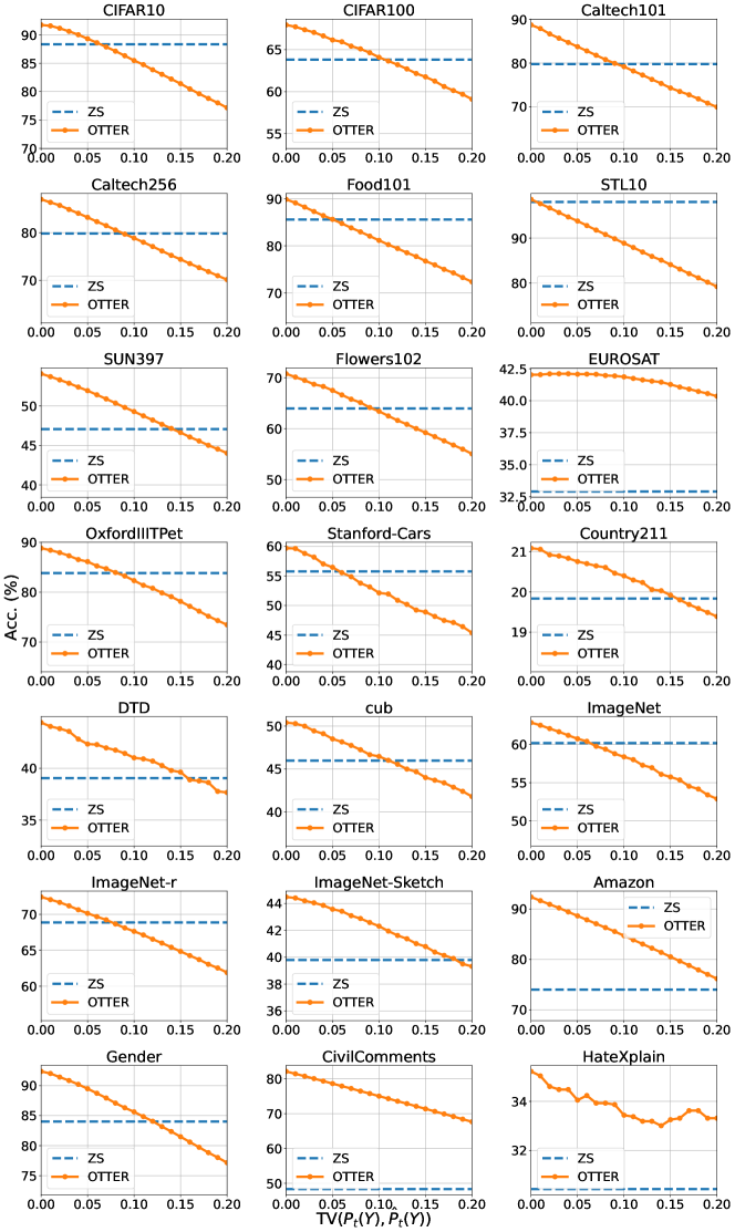
Figure 4: Ablation experiment on the class balance specification. X-axis represents the total variation distance between the class specification true class balance $P_{t}(Y)$ and $\hat{P}_{t}(Y)$. Y-axis represents accuracy. ViT-B/16 is used as the image zero-shot classifier, and BERT is used as the text zero-shot classifier.

Inference time comparison

To show that the additional computation complexity induced by OTTER is not heavy, we measured the time consumption (in seconds) for the inference step in the experiments in Section 5.2, with the pre-computed embeddings. Table 11 presents the result. Time reduction column represents the time reduction rate of OTTER compared to PM. Measurements were taken using a machine equipped with an Intel® Core™ i7-11700K @ 3.60GHz processor, 64GB RAM, and NVIDIA GPU RTX-4090. For most cases (n<30000), our method takes less than 1 second, while the prior matching baseline takes more than 3 seconds. It’s worth noting that the time consumption for computing embeddings is more substantial; even 10 seconds is negligible compared to the embedding time consumption (ranging from 5 to 30 minutes for each evaluation set), which is common for all inference conditions.

Dataset	n	ZS	PM	OTTER	Time reudction (%)
CIFAR10	10000	0.0381	3.7127	0.0733	98.03
CIFAR100	10000	0.0462	3.6296	0.1947	94.64
Caltech101	7162	0.0298	3.6445	0.1188	96.74
Caltech256	22897	0.2111	3.9597	0.8568	78.36
Food101	25250	0.1186	3.6968	0.4969	86.56
STL10	8000	0.0304	3.4877	0.0546	98.43
SUN397	87004	1.1233	33.0386	10.5316	68.12
Flowers102	6149	0.0280	3.7216	0.0959	97.42
EuroSAT	22000	0.0826	3.6655	0.3491	90.48
OXFORD-IIIT-Pet	3669	0.0137	3.3901	0.0233	99.31
STANFORD-Cars	8041	0.0413	3.4910	0.1964	94.37
Country211	21100	0.1285	3.7665	1.0537	72.02
DTD	1880	0.0070	3.4603	0.0156	99.55
CUB	5794	0.0306	3.5583	0.1410	96.04
ImageNet	40000	0.9954	37.6932	8.1003	78.51
ImageNet-r	26000	0.1921	3.8331	0.9834	74.35
ImageNet-Sketch	40889	1.0189	38.4853	9.0579	76.46

Table 11: Inference time comparison with pre-computed embeddings (in seconds).

Ablation on prompts

Recent studies have demonstrated the efficacy of enhancing prompts as a means to improve zero-shot models [71, 38]. In order to further illustrate the potential enhancements offered by OTTER beyond enhanced prompts, we reproduced Menon and Vondrick [38]’s approach (Classification by Description, CD), which employs multiple prompts generated by language models and takes max scores of them for each class. We applied OTTER to CD. The results of this experiment are summarized in Table 12. As anticipated, OTTER exhibits enhancements in zero-shot classification, even when prompt sets are refined using language models.

	ZS	PM	OT	ZS + CD	PM + CD	OT + CD
EuroSAT	32.90	11.36	42.03	53.62	11.37	57.15
Oxford-IIIT-Pet	83.84	23.11	88.83	87.95	16.33	91.01
DTD	39.04	8.83	44.41	42.87	14.73	43.24
CUB	45.98	10.34	50.40	55.51	11.49	58.47
ImageNet	60.18	12.42	62.86	66.46	14.08	68.05

Table 12: Accuracy in the prompt-enhanced zero-shot classification by Classification by Description (CD) [38]. We can observe OTTER’s capability to provide further enhancements upon refined the improvements achieved through refined prompts.

D.4 Detailed experiment results of Section 5.2.2

Class balance estimation errors

We report the class balance errors in Section 5.2.2. As a metric, we use the total variance $TV(\nu,\hat{\nu})=\frac{1}{2}\left|\left|\nu-\hat{\nu}\right|\right|_{1}$. We use zeroshot prediction scores and linear probing prediction scores for BBSE. $\hat{\nu}^{zs}$ denotes the estimated class balance based on zero-shot prediction scores, and $\hat{\nu}^{lp}$ represents the estimated class balance based on linear probing prediction scores.

Table 13 shows the result. We can see that total variation decreases with linear probing in image classification tasks since they reduces the violation of label shift assumptions. However, total variation increases in text classification tasks due to the small number of labeled sample size, following the size of label space ($K=2$ or $3$). Accordingly, we can expect OTTER will be more useful with linear probing, and just rebalancing zero-shot predictions with OTTER could be enough for text classification tasks.

Dataset	TV($\nu^{*},\hat{\nu}^{zs}$)	TV($\nu^{*},\hat{\nu}^{lp}$)	Dataset	TV($\nu^{*},\hat{\nu}^{zs}$)	TV($\nu^{*},\hat{\nu}^{lp}$)
CIFAR10	0.071	0.038	STL10	0.021	0.011
CIFAR100	0.219	0.153	SUN397	0.503	0.458
Caltech101	0.130	0.041	CUB	0.245	0.102
Caltech256	0.126	0.081	ImageNet	0.175	0.175
Country211	0.439	0.336	ImageNet-r	0.210	0.189
DTD	0.441	0.160	ImageNet-sketch	0.236	0.211
EUROSAT	0.404	0.084	Amazon	0.090	0.253
Flowers102	0.202	0.067	CivilComments	0.369	0.383
Food101	0.112	0.090	Gender	0.083	0.155
Oxford-IIIT-Pet	0.219	0.114	HateXplain	0.253	0.203
Stanford-Cars	0.255	0.143

Table 13: Class balance estimation error with BBSE in Section 5.2.2. We report the mean of 10 different random samplings of the validation set. Lower is better.

Ablation experiments on linear probing

We provide full results of Section 5.2.2. Specifically, we additionally report the results of combination with linear probing in text classification tasks and the results of zero-shot classification results in image classification tasks.

The results are presented in Table 14. While OTTER often provides additional improvement over LP, zero-shot classification was a strong baseline in image classification tasks. Meanwhile, class balance adaptation in text classification tasks is effective in all cases, giving a significant improvement over zero-shot predictions.

Dataset	ZS	ZS BBSE+PM	ZS BBSE+OT	LP	LP BBSE+PM	LP BBSE+OT
CIFAR10	88.3	72.7	87.5	90.2	89.8	90.0
CIFAR100	63.8	3.2	59.1	58.3	24.4	60.5
Caltech101	79.8	32.5	80.7	91.5	87.5	91.4
Caltech256	79.8	6.0	80.3	84.5	58.4	85.4
Country211	19.8	1.5	15.9	12.4	9.2	13.2
DTD	39.0	3.2	31.2	58.6	49.0	59.3
EUROSAT	32.9	19.2	34.0	74.6	71.6	75.9
Flowers102	64.0	40.3	60.8	89.0	87.8	90.2
Food101	85.6	15.3	82.3	79.1	60.6	79.8
Oxford-IIIT-Pet	83.8	43.3	71.4	75.7	72.0	75.6
Stanford-Cars	55.7	2.3	51.7	64.5	65.4	66.3
STL10	98.0	97.4	96.9	97.7	97.5	97.6
SUN397	47.1	6.9	25.6	0.2	0.2	0.2
cub	46.0	3.3	45.5	72.2	63.3	75.6
ImageNet	60.2	0.8	57.7	56.8	53.6	59.8
ImageNet-r	68.9	1.7	63.3	54.9	47.6	57.1
ImageNet-Sketch	39.8	0.8	40.4	43.4	37.9	48.3
Amazon	74.0	47.9	89.1	71.3	66.9	71.3
CivilComments	48.3	69.1	55.8	53.8	45.5	53.8
Gender	84.0	57.0	87.8	78.0	71.2	78.5
HateXplain	30.4	34.4	35.2	32.8	32.7	32.3

Table 14: Accuracy (%) with OTTER combined with class balance estimation. ZS BBSE denotes BBSE class balance estimation based on zero-shot prediction scores, and LP BBSE denotes BBSE class balance estimation based on linear probing prediction scores. We report the mean of 10 different random samplings of the validation set.

Ablation experiments on the number of examples per class

Few-shot adaptation scenario assumes we have access to labeled data to estimate the target distribution. We hypothesize that an increase in the number of labeled samples enhances the accuracy of the class balance estimation, thereby improving the performance of OTTER. To test this hypothesis, we use few-shot adaptation in image and text classification tasks, without linear probing. The experiment varies the number of samples per class from 10 to 100, anticipating a reduction in class balance estimation error and an improvement in OTTER’s accuracy with the increase in labeled samples.

The results, as depicted in Figure 5, corroborate our hypothesis. It is evident that the error in class balance estimation diminishes with an increasing number of samples, leading to a concurrent enhancement in the accuracy of OTTER.

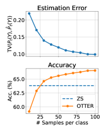
(a)

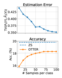
(b)

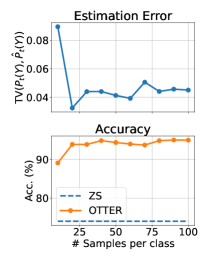
(c)

(d)

Figure 5: Ablation experiment on the number of samples. We report the mean of 10 different samplings in each setting. We use ViT-B/16 for image classification, and BERT for text classification.

Comparison between OTTER and Linear Probing with varying number of classes

In the few-shot adaptation scenario, we explored three approaches: OTTER, linear probing (LP), and a combination of LP + OTTER. We formulated two hypotheses. The first posits that OTTER might outperform LP, particularly in situations with a limited number of samples. The second hypothesis suggests that OTTER could provide further enhancements to LP even when LP already surpasses the naive version of OTTER. This experiment was conducted using the same setup as the previous one.

The results, displayed in Figure 6, reveal several insights regarding our hypotheses. To begin with, OTTER demonstrates performance on par with LP, especially in scenarios with fewer samples. Interestingly, OTTER achieves superior accuracy compared to LP in datasets like Amazon and CivilComments, characterized by a small number of classes ($K=2$), resulting in a relatively low total sample count. Furthermore, it is observed that incorporating OTTER into LP leads to an average increase in accuracy.

(a)

(b)

(c)

(d)

Figure 6: Comparison between OTTER, LP, and LP+OTTER with varying the number of samples. We report the mean of 10 different samplings in each setting. We use ViT-B/16 for image classification, and BERT for text classification.

D.5 Detailed experiment setup and results of Section 5.2.3

Class hierarchy

We used the following superclasses and subclasses classes for the proof of concept.

• fish: aquarium fish, flatfish, ray, shark , trout

• tree: maple tree, oak tree, palm tree, pine tree, willow tree

Class balance estimation error

We report the class balance estimation error in Section 5.2.3. Table 15 shows the total variation between true class balance and estimated class balance. We can expect a significant accuracy improvement for RN50, RN101, and ViT-B/16 based on this table.

	BBSE	H-BBSE
RN50	0.335	0.246
RN101	0.378	0.294
ViT-B/32	0.156	0.167
ViT-B/16	0.287	0.246
ViT-L/14	0.131	0.152

Table 15: Class balance estimation error in the Section 5.2.3 experiment. Class balance estimation error is measured by total variation distance. We report the mean of 10 different samplings of the validation set. H-BBSE denotes the class balance estimation using hierarchy upon BBSE.

References

- Adila et al. [2023] Dyah Adila, Changho Shin, Linrong Cai, and Frederic Sala. Zero-shot robustification of zero-shot models with foundation models. arXiv preprint arXiv:2309.04344, 2023.
- Agarwal et al. [2021] Sandhini Agarwal, Gretchen Krueger, Jack Clark, Alec Radford, Jong Wook Kim, and Miles Brundage. Evaluating clip: towards characterization of broader capabilities and downstream implications. arXiv preprint arXiv:2108.02818, 2021.
- Alexandari et al. [2020] Amr Alexandari, Anshul Kundaje, and Avanti Shrikumar. Maximum likelihood with bias-corrected calibration is hard-to-beat at label shift adaptation. In International Conference on Machine Learning, pages 222–232. PMLR, 2020.
- An et al. [2023] Bang An, Sicheng Zhu, Michael-Andrei Panaitescu-Liess, Chaithanya Kumar Mummadi, and Furong Huang. More context, less distraction: Visual classification by inferring and conditioning on contextual attributes. arXiv preprint arXiv:2308.01313, 2023.
- Azé and Corvellec [2002] Dominique Azé and Jean-Noël Corvellec. On the sensitivity analysis of hoffman constants for systems of linear inequalities. SIAM Journal on Optimization, 12(4):913–927, 2002.
- Azizzadenesheli et al. [2019] Kamyar Azizzadenesheli, Anqi Liu, Fanny Yang, and Animashree Anandkumar. Regularized learning for domain adaptation under label shifts. In International Conference on Learning Representations, 2019.
- Borkan et al. [2019] Daniel Borkan, Lucas Dixon, Jeffrey Sorensen, Nithum Thain, and Lucy Vasserman. Nuanced metrics for measuring unintended bias with real data for text classification. In Companion proceedings of the 2019 world wide web conference, pages 491–500, 2019.
- Bossard et al. [2014] Lukas Bossard, Matthieu Guillaumin, and Luc Van Gool. Food-101–mining discriminative components with random forests. In Computer Vision–ECCV 2014: 13th European Conference, Zurich, Switzerland, September 6-12, 2014, Proceedings, Part VI 13, pages 446–461. Springer, 2014.
- Chang et al. [2022] Wanxing Chang, Ye Shi, Hoang Tuan, and Jingya Wang. Unified optimal transport framework for universal domain adaptation. Advances in Neural Information Processing Systems, 35:29512–29524, 2022.
- Chang et al. [2015] Xiaojun Chang, Yi Yang, Alexander G. Hauptmann, Eric P. Xing, and Yao-Liang Yu. Semantic concept discovery for large-scale zero-shot event detection. In Proceedings of the 24th International Conference on Artificial Intelligence, IJCAI’15, page 2234–2240. AAAI Press, 2015. ISBN 9781577357384.
- Chawla et al. [2002] Nitesh V Chawla, Kevin W Bowyer, Lawrence O Hall, and W Philip Kegelmeyer. Smote: synthetic minority over-sampling technique. Journal of artificial intelligence research, 16:321–357, 2002.
- Chuang et al. [2023] Ching-Yao Chuang, Varun Jampani, Yuanzhen Li, Antonio Torralba, and Stefanie Jegelka. Debiasing vision-language models via biased prompts. arXiv preprint arXiv:2302.00070, 2023.
- Cimpoi et al. [2014] Mircea Cimpoi, Subhransu Maji, Iasonas Kokkinos, Sammy Mohamed, and Andrea Vedaldi. Describing textures in the wild. In Proceedings of the IEEE conference on computer vision and pattern recognition, pages 3606–3613, 2014.
- Coates et al. [2011] Adam Coates, Andrew Ng, and Honglak Lee. An analysis of single-layer networks in unsupervised feature learning. In Proceedings of the fourteenth international conference on artificial intelligence and statistics, pages 215–223. JMLR Workshop and Conference Proceedings, 2011.
- Dalton et al. [2013] Jeffrey Dalton, James Allan, and Pranav Mirajkar. Zero-shot video retrieval using content and concepts. In Proceedings of the 22nd ACM International Conference on Information & Knowledge Management, CIKM ’13, page 1857–1860, New York, NY, USA, 2013. Association for Computing Machinery. ISBN 9781450322638. doi: 10.1145/2505515.2507880. URL https://doi.org/10.1145/2505515.2507880.
- Deng et al. [2009] Jia Deng, Wei Dong, Richard Socher, Li-Jia Li, Kai Li, and Li Fei-Fei. Imagenet: A large-scale hierarchical image database. In 2009 IEEE conference on computer vision and pattern recognition, pages 248–255. Ieee, 2009.
- Devlin et al. [2018] Jacob Devlin, Ming-Wei Chang, Kenton Lee, and Kristina Toutanova. Bert: Pre-training of deep bidirectional transformers for language understanding. arXiv preprint arXiv:1810.04805, 2018.
- Dinan et al. [2020] Emily Dinan, Angela Fan, Ledell Wu, Jason Weston, Douwe Kiela, and Adina Williams. Multi-dimensional gender bias classification. In Proceedings of the 2020 Conference on Empirical Methods in Natural Language Processing (EMNLP), pages 314–331, Online, November 2020. Association for Computational Linguistics. doi: 10.18653/v1/2020.emnlp-main.23. URL https://www.aclweb.org/anthology/2020.emnlp-main.23.
- Dixon et al. [2018] Lucas Dixon, John Li, Jeffrey Sorensen, Nithum Thain, and Lucy Vasserman. Measuring and mitigating unintended bias in text classification. 2018.
- Fei-Fei et al. [2006] Li Fei-Fei, Robert Fergus, and Pietro Perona. One-shot learning of object categories. IEEE transactions on pattern analysis and machine intelligence, 28(4):594–611, 2006.
- Fernández et al. [2018] Alberto Fernández, Salvador García, Mikel Galar, Ronaldo C Prati, Bartosz Krawczyk, and Francisco Herrera. Learning from imbalanced data sets, volume 10. Springer, 2018.
- Garg et al. [2020] Saurabh Garg, Yifan Wu, Sivaraman Balakrishnan, and Zachary Lipton. A unified view of label shift estimation. Advances in Neural Information Processing Systems, 33:3290–3300, 2020.
- Griffin et al. [2007] Gregory Griffin, Alex Holub, and Pietro Perona. Caltech-256 object category dataset. 2007.
- Guo et al. [2022] Dandan Guo, Zhuo Li, He Zhao, Mingyuan Zhou, Hongyuan Zha, et al. Learning to re-weight examples with optimal transport for imbalanced classification. Advances in Neural Information Processing Systems, 35:25517–25530, 2022.
- He et al. [2023] Jianfeng He, Julian Salazar, Kaisheng Yao, Haoqi Li, and Jinglun Cai. Zero-shot end-to-end spoken language understanding via cross-modal selective self-training. arXiv preprint arXiv:2305.12793, 2023.
- Helber et al. [2019] Patrick Helber, Benjamin Bischke, Andreas Dengel, and Damian Borth. Eurosat: A novel dataset and deep learning benchmark for land use and land cover classification. IEEE Journal of Selected Topics in Applied Earth Observations and Remote Sensing, 12(7):2217–2226, 2019.
- Hendrycks et al. [2021] Dan Hendrycks, Steven Basart, Norman Mu, Saurav Kadavath, Frank Wang, Evan Dorundo, Rahul Desai, Tyler Zhu, Samyak Parajuli, Mike Guo, et al. The many faces of robustness: A critical analysis of out-of-distribution generalization. In Proceedings of the IEEE/CVF International Conference on Computer Vision, pages 8340–8349, 2021.
- Hoffman [1952] Alan J Hoffman. On approximate solutions of systems of linear inequalities. Journal of Research of the National Bureau of Standards, 49(4), 1952.
- Kahana et al. [2022] Jonathan Kahana, Niv Cohen, and Yedid Hoshen. Improving zero-shot models with label distribution priors. arXiv preprint arXiv:2212.00784, 2022.
- Krause et al. [2013] Jonathan Krause, Michael Stark, Jia Deng, and Li Fei-Fei. 3d object representations for fine-grained categorization. In Proceedings of the IEEE international conference on computer vision workshops, pages 554–561, 2013.
- Krizhevsky et al. [2009] Alex Krizhevsky, Geoffrey Hinton, et al. Learning multiple layers of features from tiny images. 2009.
- Lipton et al. [2018a] Zachary Lipton, Yu-Xiang Wang, and Alexander Smola. Detecting and correcting for label shift with black box predictors. In International conference on machine learning, pages 3122–3130. PMLR, 2018a.
- Lipton et al. [2018b] Zachary Lipton, Yu-Xiang Wang, and Alexander Smola. Detecting and correcting for label shift with black box predictors. In International conference on machine learning, pages 3122–3130. PMLR, 2018b.
- Liu et al. [2023] Haotian Liu, Chunyuan Li, Qingyang Wu, and Yong Jae Lee. Visual instruction tuning. arXiv preprint arXiv:2304.08485, 2023.
- Liusie et al. [2023] Adian Liusie, Potsawee Manakul, and Mark JF Gales. Mitigating word bias in zero-shot prompt-based classifiers. arXiv preprint arXiv:2309.04992, 2023.
- Loshchilov and Hutter [2018] Ilya Loshchilov and Frank Hutter. Decoupled weight decay regularization. In International Conference on Learning Representations, 2018.
- Mathew et al. [2021] Binny Mathew, Punyajoy Saha, Seid Muhie Yimam, Chris Biemann, Pawan Goyal, and Animesh Mukherjee. Hatexplain: A benchmark dataset for explainable hate speech detection. In Proceedings of the AAAI Conference on Artificial Intelligence, volume 35, pages 14867–14875, 2021.
- Menon and Vondrick [2022] Sachit Menon and Carl Vondrick. Visual classification via description from large language models. arXiv preprint arXiv:2210.07183, 2022.
- Nam et al. [2021] Jinwoo Nam, Daechul Ahn, Dongyeop Kang, Seong Jong Ha, and Jonghyun Choi. Zero-shot natural language video localization. In Proceedings of the IEEE/CVF International Conference on Computer Vision, pages 1470–1479, 2021.
- Ni et al. [2019] Jianmo Ni, Jiacheng Li, and Julian McAuley. Justifying recommendations using distantly-labeled reviews and fine-grained aspects. In Proceedings of the 2019 conference on empirical methods in natural language processing and the 9th international joint conference on natural language processing (EMNLP-IJCNLP), pages 188–197, 2019.
- Nilsback and Zisserman [2008] Maria-Elena Nilsback and Andrew Zisserman. Automated flower classification over a large number of classes. In 2008 Sixth Indian conference on computer vision, graphics & image processing, pages 722–729. IEEE, 2008.
- Novack et al. [2023] Zachary Novack, Julian McAuley, Zachary Chase Lipton, and Saurabh Garg. Chils: Zero-shot image classification with hierarchical label sets. In International Conference on Machine Learning, pages 26342–26362. PMLR, 2023.
- Parkhi et al. [2012] Omkar M Parkhi, Andrea Vedaldi, Andrew Zisserman, and CV Jawahar. Cats and dogs. In 2012 IEEE conference on computer vision and pattern recognition, pages 3498–3505. IEEE, 2012.
- Pena et al. [2021] Javier Pena, Juan C Vera, and Luis F Zuluaga. New characterizations of hoffman constants for systems of linear constraints. Mathematical Programming, 187:79–109, 2021.
- Peña [2024] Javier F Peña. An easily computable upper bound on the hoffman constant for homogeneous inequality systems. Computational Optimization and Applications, 87(1):323–335, 2024.
- Peng et al. [2021] Hanyu Peng, Mingming Sun, and Ping Li. Optimal transport for long-tailed recognition with learnable cost matrix. In International Conference on Learning Representations, 2021.
- Peyré et al. [2019] Gabriel Peyré, Marco Cuturi, et al. Computational optimal transport: With applications to data science. Foundations and Trends® in Machine Learning, 11(5-6):355–607, 2019.
- Radford et al. [2021] Alec Radford, Jong Wook Kim, Chris Hallacy, Aditya Ramesh, Gabriel Goh, Sandhini Agarwal, Girish Sastry, Amanda Askell, Pamela Mishkin, Jack Clark, et al. Learning transferable visual models from natural language supervision. In International conference on machine learning, pages 8748–8763. PMLR, 2021.
- Reed et al. [2016] S. Reed, Z. Akata, H. Lee, and B. Schiele. Learning deep representations of fine-grained visual descriptions. In 2016 IEEE Conference on Computer Vision and Pattern Recognition (CVPR), pages 49–58, Los Alamitos, CA, USA, jun 2016. IEEE Computer Society. doi: 10.1109/CVPR.2016.13. URL https://doi.ieeecomputersociety.org/10.1109/CVPR.2016.13.
- Reimers and Gurevych [2019] Nils Reimers and Iryna Gurevych. Sentence-bert: Sentence embeddings using siamese bert-networks. arXiv preprint arXiv:1908.10084, 2019.
- Ren et al. [2016] Zhou Ren, Hailin Jin, Zhe Lin, Chen Fang, and Alan Yuille. Joint image-text representation by gaussian visual-semantic embedding. In Proceedings of the 24th ACM International Conference on Multimedia, MM ’16, page 207–211, New York, NY, USA, 2016. Association for Computing Machinery. ISBN 9781450336031. doi: 10.1145/2964284.2967212. URL https://doi.org/10.1145/2964284.2967212.
- Roberts et al. [2023] Nicholas Roberts, Xintong Li, Dyah Adila, Sonia Cromp, Tzu-Heng Huang, Jitian Zhao, and Frederic Sala. Geometry-aware adaptation for pretrained models. In Thirty-seventh Conference on Neural Information Processing Systems, 2023.
- Robinson [1973] Stephen M Robinson. Bounds for error in the solution set of a perturbed linear program. Linear Algebra and its applications, 6:69–81, 1973.
- Sain et al. [2023] Aneeshan Sain, Ayan Kumar Bhunia, Pinaki Nath Chowdhury, Subhadeep Koley, Tao Xiang, and Yi-Zhe Song. Clip for all things zero-shot sketch-based image retrieval, fine-grained or not. In Proceedings of the IEEE/CVF Conference on Computer Vision and Pattern Recognition, pages 2765–2775, 2023.
- Saito et al. [2023] Kuniaki Saito, Kihyuk Sohn, Xiang Zhang, Chun-Liang Li, Chen-Yu Lee, Kate Saenko, and Tomas Pfister. Pic2word: Mapping pictures to words for zero-shot composed image retrieval. In Proceedings of the IEEE/CVF Conference on Computer Vision and Pattern Recognition, pages 19305–19314, 2023.
- Santambrogio [2015] Filippo Santambrogio. Optimal transport for applied mathematicians. Birkäuser, NY, 55(58-63):94, 2015.
- Sato et al. [2023] Fumiaki Sato, Ryo Hachiuma, and Taiki Sekii. Prompt-guided zero-shot anomaly action recognition using pretrained deep skeleton features. In Proceedings of the IEEE/CVF Conference on Computer Vision and Pattern Recognition, pages 6471–6480, 2023.
- Shi et al. [2024] Liangliang Shi, Haoyu Zhen, Gu Zhang, and Junchi Yan. Relative entropic optimal transport: a (prior-aware) matching perspective to (unbalanced) classification. Advances in Neural Information Processing Systems, 36, 2024.
- Tachet des Combes et al. [2020] Remi Tachet des Combes, Han Zhao, Yu-Xiang Wang, and Geoffrey J Gordon. Domain adaptation with conditional distribution matching and generalized label shift. Advances in Neural Information Processing Systems, 33:19276–19289, 2020.
- Tai et al. [2021] Kai Sheng Tai, Peter D Bailis, and Gregory Valiant. Sinkhorn label allocation: Semi-supervised classification via annealed self-training. In International Conference on Machine Learning, pages 10065–10075. PMLR, 2021.
- Thai-Nghe et al. [2010] Nguyen Thai-Nghe, Zeno Gantner, and Lars Schmidt-Thieme. Cost-sensitive learning methods for imbalanced data. In The 2010 International joint conference on neural networks (IJCNN), pages 1–8. IEEE, 2010.
- Torralba and Efros [2011] Antonio Torralba and Alexei A. Efros. Unbiased look at dataset bias. In CVPR 2011, pages 1521–1528, 2011. doi: 10.1109/CVPR.2011.5995347.
- Wah et al. [2011] Catherine Wah, Steve Branson, Peter Welinder, Pietro Perona, and Serge Belongie. The caltech-ucsd birds-200-2011 dataset. 2011.
- Wang et al. [2022] Haobo Wang, Mingxuan Xia, Yixuan Li, Yuren Mao, Lei Feng, Gang Chen, and Junbo Zhao. Solar: Sinkhorn label refinery for imbalanced partial-label learning. Advances in Neural Information Processing Systems, 35:8104–8117, 2022.
- Wang et al. [2019] Haohan Wang, Songwei Ge, Zachary Lipton, and Eric P Xing. Learning robust global representations by penalizing local predictive power. Advances in Neural Information Processing Systems, 32, 2019.
- Wei et al. [2021] Jason Wei, Maarten Bosma, Vincent Y Zhao, Kelvin Guu, Adams Wei Yu, Brian Lester, Nan Du, Andrew M Dai, and Quoc V Le. Finetuned language models are zero-shot learners. arXiv preprint arXiv:2109.01652, 2021.
- Xian et al. [2023] Ruicheng Xian, Lang Yin, and Han Zhao. Fair and optimal classification via post-processing. 2023.
- Xiao et al. [2010] Jianxiong Xiao, James Hays, Krista A Ehinger, Aude Oliva, and Antonio Torralba. Sun database: Large-scale scene recognition from abbey to zoo. In 2010 IEEE computer society conference on computer vision and pattern recognition, pages 3485–3492. IEEE, 2010.
- Yazdani and Henderson [2015] Majid Yazdani and James Henderson. A model of zero-shot learning of spoken language understanding. pages 244–249, 01 2015. doi: 10.18653/v1/D15-1027.
- Zhang et al. [2024] Chuyu Zhang, Hui Ren, and Xuming He. P2ot: Progressive partial optimal transport for deep imbalanced clustering. arXiv preprint arXiv:2401.09266, 2024.
- Zhou et al. [2022] Kaiyang Zhou, Jingkang Yang, Chen Change Loy, and Ziwei Liu. Learning to prompt for vision-language models. International Journal of Computer Vision, 130(9):2337–2348, 2022.