Superbunched radiation of a tunnel junction due to charge quantization
Steven Kim and Fabian Hassler
Institute for Quantum Information, RWTH Aachen University, 52056 Aachen, Germany
(April 12, 2024)
Abstract
A chaotic light source is characterized by the fact that many independent emitters radiate photons with a random optical phase.
This is similar compared to a tunnel junction where many independent channels are able to emit photons due to a coupling to an electromagnetic environment.
However, in a recent experiment it has been observed that a tunnel junction can deviate from the expectation of chaotic light and is able to emit strongly correlated, superbunched photons.
Motivated by this, we study the correlation of the radiation and show that the superbunching originates from the emission of multiple photons which is possible due to the quantization of charge.
Introduction.—Electrons at low temperature that traverse a constriction biased at a finite voltage are able to emit photons up to a frequency due to a coupling to an electromagnetic environment [1].
Microscopically, this radiation is emitted due to current fluctuations arising from shot-noise caused by the partitioning at the constriction [2].
For a quantum point contact, the electron transport is anti-bunched [3].
It has been shown that for a single transport channel this correlation can be transferred to the emitted photons [4, 5, 6].
The correlation of the photons is encoded in the second-order coherence [ the annihilation operator of a photon at time ]
(1)
describing the correlation between an initially emitted photon and a photon at a later time , where indicates anti-bunching [7].
However, due to their bosonic nature photons are typically bunched with .
In fact, a broad class of light sources emit so called ‘chaotic light’ that exhibit the special value of [8].
Chaotic light is realized in a situation where many independent emitters radiate photons with random optical phases.
At first sight, a tunnel junction, i.e., a constriction with many channels where all the transmission probabilities , is expected to produce chaotic light [9, 10].
This is due to the fact that the electron transport in different channels are independent, the transmission of electrons is rare and Poissonian, and the optical phase of the emitted radiation is random.
However, a recent experiment [11] has shown that a tunnel junction can act as a source of highly correlated light with , dubbed ‘superbunching’ [12, 13].
Motivated by this result, we theoretically study the correlation of the radiation emitted by a tunnel junction.
Here, we show that a tunnel junction acts as a chaotic light source only for weak light-matter interaction.
At stronger interaction, superbunching of photons is predicted by processes where a single electron emits a cascade of multiple photons.
On a fundamental level, the emission of a cascade of photons originates from the quantization of charge making the transport of electrons a point process [14, 15].
For a voltage , a single electron is able to emit up to photons in a single event which is reflected in a large value of .
Note that cascade effects leading to bunching have been studied before in the context of electron transport in molecules [16, 17, 18].
Similar effects have been studied in voltage biased Josephson junctions where a single Cooper pair can emit multiple photons while tunneling [19, 20, 21].
Note, however, that in the superconducting context the phase of the emitted photons is locked to the phase of the superconducting condensate such that a superconducting junction does not serve as a chaotic light source even at weak light-matter interaction.
The article is organized as follows.
We start by introducing the model and employ a Keldysh path integral approach to take the interaction with an environment into account.
After expanding the action of the path integral in the tunnel limit , we perform a rotating wave approximation (RWA) and obtain a Lindblad master equation that describes the non-unitary time evolution of the density matrix of the resonator.
From this, we determine the stationary state and the second-order coherence.
We show regimes where the second-order coherence exceeds the chaotic value of , discuss the impact of temperature, and point out that the strong correlations arise due to the quantization of charge.
The model.—
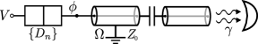
Figure 1: The setup is composed of a voltage biased tunnel junction with transmission probabilities in series with a microwave resonator that is capacitively coupled to a transmission line for readout purposes. The microwave resonator is at frequency with characteristic impedance . The variable is the node flux describing the voltage over the resonator. The transmission line introduces damping; where the photons are lost at rate into the detector.
We study the setup displayed in Fig. 1.
It consists of a resonator with the resonance frequency and the characteristic impedance .
The voltage across the resonator is given by the time-derivative of the node flux .
Due to the capacitive coupling to a readout transmission line, the photons are lost at a rate .
Close to the resonance frequency , the impedance of the resonator is given by
(2)
The resonator is in series with a tunnel junction that is biased with a DC voltage . The junction is modelled by a left (L) and right (R) electronic reservoir with the Hamiltonian
(3)
here, denotes the velocity of the fermionic mode of the -th transport channel 111The index in particular includes spin which allows the tunneling probability to depend on spin.. The leads are coupled by the tunneling Hamiltonian
(4)
where the coupling is connected to the tunneling probability [23]. Due to the DC voltage bias, the electrons in the leads are distributed as and with the Fermi-Dirac distribution at temperature with the Boltzmann constant .
The factor in the tunneling Hamiltonian is due to the finite-voltage across the resonator.
We want to derive an effective description for describing the resonator mode by integrating over the electrons with Hamiltonian .
For this, we employ a Keldysh path-integral approach. The time evolution of the density matrix of the system is given by ; here the Keldysh label [] refers to the forward [backward] propagation to the left [right] of the density matrix [24].
The action consists of a lead part
(5)
where and .
The matrices are given by
(6)
In Fourier space , the retarded [advanced] Greens function read and the Keldysh Greens function .
The tunneling contribution is given by .
The action is quadratic in and, thus, it is possible to perform the Gaussian integral over the fermionic degrees of freedom to obtain an effective action for the bosonic field [25].
Because the tunnel probabilities in a tunnel junction are small, we expand the action in the first non-vanishing order .
This yields the tunneling action [23]
(7)
where we have introduced the Keldysh rotated variables , .
All transmission channels contribute independently to the action by the total transmission probability .
It connects to the DC current through the device via the Landauer formula , i.e., the conductance is given by .
Note that the current through the tunnel junction is Poissonian such that no intrinsic electronic correlations can be transferred to the photons.
The last term of the action is due to the shot-noise with the noise-power
(8)
at frequency [26, 27, 3].
The origin is the granularity of the electron charge, as realized by Schottky [28], which is the vital ingredient that allows to produce superbunched radiation, see below.
For the dynamics of the resonator, we assume a large quality factor which allows a RWA with where is a slowly varying complex variable with phase .
To perform the RWA, we make use of the Jacobi-Anger expansion with the Bessel functions of the first kind .
After the RWA, it is possible to show [29] that the Keldysh action is equivalent to a Lindblad master equation with the Liouvillian
(9)
,dissipators , and describes the strength of the light-matter coupling, see [30] for details.
The rates depend on the Bose-Einstein distribution and describe the unsymmetrized shot-noise power, connecting to (8) via .
For [ they describe emission [absorption] of energy by the conductor [1, 31, 32].
At zero temperature, only if .
At finite temperature the rate can be non-zero also for .
But, this is suppressed because in this case.
Note that in Refs. [33, 34], it has been shown that over-bias emission of photons is also possible at zero temperature.
However, this is due to co-tunneling and thus a higher-order process that scales with [35].
The jump operators are given by ( is the confluent hypergeometric function)
(10)
where the colons denote normal ordering (all creation operators to the left of the annihilation operators ).
To lowest order in the light-matter coupling , the jump operators are given by and thus describe the creation [absorption] of photons [] in the resonator by a cascade.
Besides the creation and annihilation of photons, the jump operators also include higher order dynamics due to that appear at elevated light-matter interaction .
Physically, these corrections arise due to the backaction of the resonator onto the tunnel junction when the voltage across the resonator becomes finite and impacts the voltage across the junction.
This backaction can be exploited to achieve a single photon source with [36, 37, 15].
Note, however, that due to the chirality of quantum hall edge channels it is possible to suppress the backaction such that for all [38].
This is beneficiary for the oberservation of superbunching, see below.
The last ingredient of the modelling is the coupling of the resonator to the detector with rate and at temperature .
It leads to the absorption and emission of photons given by the Liouvillian
(11)
with , see e.g. [39].
The time-evolution of the density matrix of the resonator is thus given by .
It incorporates both the interaction of the resonator with the tunnel junction and the detector.
Note that the phase of the emitted photons of the resonator is arbitrary which is due to the -symmetry of the Liouvillian [40].
In this sense, the system consists of many independent sources given by the different channels that emit radiation with a random optical phase.
Still, we will observe superbunching of the radiation due to the fact that the electronic charge is granular.
Second-order coherence.—The second-order coherence quantifies the correlation of photons.
For chaotic light, it can be shown that [8].
Such light sources include blackbody radiation and emission from an Ohmic resistor, see below.
We determine the value of the second-order coherence for our system by solving for the stationary density matrix , fulfilling .
The second-order coherence can then be obtained by with .
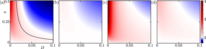
Figure 2:
Second-order coherence as a function of the light-matter coupling and conductance for (up to 2 photon process possible) in (a) and (b) and for (up to 4 photon process possible) in (c) and (d); with and [] in (a),(c) [in (b),(d)]. The superbunched region is indicated in red.
Note that in (c) values up to are present (the colorbar is maxed out at 4 for better visibility). The black line in (a) indicates the transition line at zero temperature; at finite temperature, the region of superbunching is larger. In general for larger voltages, both the region of superbunching as well as the values of are increased.
Results for the second-order coherence obtained by a numerical simulation are shown in Fig. 2 for different parameters.
It can be seen that especially at low-temperature, small, and large voltages superbunched radiation with is produced.
The smallness of the transmission is required such that the superbunching events are rare and separate in time.
Additionally, the light-matter interaction has to be sufficiently large such that multi-photon processes are present at all [19].
We would like to obtain further analytical insights into the superbunching effect.
For the following, we concentrate on zero temperature () and choose a voltage with such that only one- and two-photon cascade events corresponding to are relevant.
First, we focus on the one-photon dynamics.
In this situation, single photons are lost with a rate while they are predominantely generated by the jump operator with the rate .
For convenience, we assume that and small which is fulfilled in the relevant part of Fig. 2.
In this regime, we have that and thus the mean photon number in the resonator .
Additionally for small , we have which yields from (10).
The approximate Liouvillian in this case is given by which yields the Gaussian contribution since it is quadratic in and .
The stationary state is an effective thermal state with average occupation .
Because of this, we have to this order.
Note that the Liouvillian is also obtained for the situation of an Ohmic resistor when the discreteness of charge can be neglected such that .
This shows that the superbunched radiation is a property of the quantization of charge such that a single electron emits a cascade of photons.
To obtain the cascade effect, we have to calculate the next order correction in .
There are two new contributions in this order.
The first arises due to the expansion of the hypergeometric function in .
The second process that is important to this order is the two photon cascade described by .
As shown in [30], the average photon number in this approximation is given by
(12)
where .
The higher order terms originate from higher orders of the Gaussian contribution , the nonlinearity of , and the two-photon cascade process .
The second-order coherence is given by
(13)
see [30] for details.
The first term [] arises due to the chaotic Gaussian contribution as described above.
At elevated and due to the emission of a cascade of photons, additional non-Gaussian contributions appear.
The second term, partially, stems form the backaction expressed by the nonlinearity of the hypergeometric function of = .
Note that it lowers the second-order coherence and counteracts the observation of superbunching.
The superbunching in this parameter regime arises due to the two-photon cascade effects described by .
It yields a large positive contribution expressed in the last term of (13) 222It also leads to a negative correction due to the fact that the photon occupation in the resonator increases. However, this effect is subdominant and simply renormalizes the effect of ..
The cascade events scale with such that the superbunching effect is strongest when the transmission events are separated in time due to a small conductance.
Then, the superbunched photons can be emitted by the resonator before a new bunch is created.
This fact remains true also at voltages where higher order cascades are possible.
The superbunching persists to finite temperatures.
In this case, the divergence in the limit is cured and the systems occupies a thermal state with the average occupation and [42].
At elevated conductance D, the behavior (13) remains unchanged.
For small temperature, the superbunching is maximal at the crossover scale with .
As a result, for the two-photon cascade with a maximal value of can be found at .
The results obtained in this work can be measured in setups, Fig. 1, operating at microwave frequencies that are already available.
Today’s experiments can achieve resonators with a characteristic impedance , frequency GHz, operated at temperatures mK [38].
This yields for the light-matter coupling and an Bose-Einstein occupation of . For these parameters at the optimal value , we obtain for the two-photon cascade.
Note that our findings provide insights into the intriguing experiment of Ref. [11] which measured at optical frequencies.
For optical wavelengths, the zero temperature result (13) is applicable which explains the large values of the second-order coherence at small with .
Due to the absence of a cavity in Ref. [11], for an estimate, we set and obtain at the experimental value .
Conclusion.—To conclude, we have studied the correlation of the emitted radiation by a tunnel junction.
Intuitively, it is expected that the tunnel junction acts as a chaotic light source because many independent channels emit photons with a random optical phase.
However, we have shown that the quantization of charge yields non-Gaussian dynamics and makes the emission of multiple photons in a cascade during a single transmission event possible.
Because of this, the photons are highly correlated and superbunching with can be observed [11].
Additionally, we have analyzed the effect of temperature on the correlation, studied the emission of photon pairs analytically, and provided numerical results for higher order processes.
The correlations peaks at a crossover between the thermal occupation of the environment and the effective thermal state due to the tunnel junction at .
While emitters with are typically considered as classical light sources, we have shown that the strong correlations arise due to quantum effects, in particular the quantization of charge.
We acknowledge valuable discussions with C. Altimiras and O. Ghazouani Gharbi.
This work was supported by the Deutsche Forschungsgemeinschaft (DFG) under Grant No. HA 7084/8–1.
References
Lesovik and Loosen [1997]G. B. Lesovik and R. Loosen, On the detection of finite-frequency current fluctuations, JETP Lett. 65, 295 (1997).
Blanter and Büttiker [2000]Y. Blanter and M. Büttiker, Shot noise in mesoscopic conductors, Phys. Rep. 336, 1 (2000).
Lesovik [1989]G. B. Lesovik, Excess quantum noise in 2D ballistic point contacts, JETP Lett. 49, 592 (1989).
Beenakker and Schomerus [2004]C. W. J. Beenakker and H. Schomerus, Antibunched Photons Emitted by a Quantum Point Contact out of Equilibrium, Phys. Rev. Lett. 93, 096801 (2004).
Lebedev et al. [2010]A. V. Lebedev, G. B. Lesovik, and G. Blatter, Statistics of radiation emitted from a quantum point contact, Phys. Rev. B 81, 155421 (2010).
Fulga et al. [2010]I. C. Fulga, F. Hassler, and C. W. J. Beenakker, Nonzero temperature effects on antibunched photons emitted by a quantum point contact out of equilibrium, Phys. Rev. B 81, 115331 (2010).
Hassler and Otten [2015]F. Hassler and D. Otten, Second-order coherence of microwave photons emitted by a quantum point contact, Phys. Rev. B 92, 195417 (2015).
Loudon [2000]R. Loudon, The Quantum Theory of Light (Oxford University Press, 2000).
Beenakker and Schomerus [2001]C. W. J. Beenakker and H. Schomerus, Counting Statistics of Photons Produced by Electronic Shot Noise, Phys. Rev. Lett. 86, 700 (2001).
Zakka-Bajjani et al. [2010]E. Zakka-Bajjani, J. Dufouleur, N. Coulombel, P. Roche, D. C. Glattli, and F. Portier, Experimental determination of the statistics of photons emitted by a tunnel junction, Phys. Rev. Lett. 104, 206802 (2010).
Leon et al. [2019]C. C. Leon, A. Rosławska, A. Grewal, O. Gunnarsson, K. Kuhnke, and K. Kern, Photon superbunching from a generic tunnel junction, Sci. Adv. 5, eaav4986 (2019).
Wei et al. [2022]C.-Q. Wei, J.-B. Liu, X.-X. Zhang, R. Zhuang, Y. Zhou, H. Chen, Y.-C. He, H.-B. Zheng, and Z. Xu, Non-Rayleigh photon statistics of superbunching pseudothermal light, Chin. Phys. B 31, 024209 (2022).
Ye et al. [2022]Z. Ye, H.-B. Wang, J. Xiong, and K. Wang, Antibunching and superbunching photon correlations in pseudo-natural light, Photon. Res. 10, 668 (2022).
Jin et al. [2015]J. Jin, M. Marthaler, and G. Schön, Electroluminescence and multiphoton effects in a resonator driven by a tunnel junction, Phys. Rev. B 91, 085421 (2015).
Estève et al. [2018]J. Estève, M. Aprili, and J. Gabelli, Quantum dynamics of a microwave resonator strongly coupled to a tunnel junction (2018), arXiv:1807.02364 [cond-mat.mes-hall] .
Koch and von Oppen [2005]J. Koch and F. von Oppen, Franck-Condon blockade and giant Fano Factors in Transport through Single Molecules, Phys. Rev. Lett. 94, 10.1103/physrevlett.94.206804 (2005).
Belzig [2005]W. Belzig, Full counting statistics of super-Poissonian shot noise in multilevel quantum dots, Phys. Rev. B 71, 161301 (2005).
Gustavsson et al. [2009]S. Gustavsson, R. Leturcq, M. Studer, I. Shorubalko, T. Ihn, K. Ensslin, D. Driscoll, and A. Gossard, Electron counting in quantum dots, Surface Science Reports 64, 191 (2009).
Ménard et al. [2022]G. C. Ménard, A. Peugeot, C. Padurariu, C. Rolland, B. Kubala, Y. Mukharsky, Z. Iftikhar, C. Altimiras, P. Roche, H. le Sueur, P. Joyez, D. Vion, D. Esteve, J. Ankerhold, and F. Portier, Emission of Photon Multiplets by a dc-Biased Superconducting Circuit, Phys. Rev. X 12, 021006 (2022).
Lang and Armour [2021]B. Lang and A. D. Armour, Multi-photon resonances in Josephson junction-cavity circuits, New J. Phys. 23, 033021 (2021).
Arndt and Hassler [2022]L. Arndt and F. Hassler, Period tripling due to Parametric Down-Conversion in Circuit QED, Phys. Rev. Lett. 128, 187701 (2022).
Note [1]The index in particular includes spin which allows the tunneling probability to depend on spin.
Eckern et al. [1984]U. Eckern, G. Schön, and V. Ambegaokar, Quantum dynamics of a superconducting tunnel junction, Phys. Rev. B 30, 6419 (1984).
Kindermann and Nazarov [2003]M. Kindermann and Y. V. Nazarov, Interaction Effects on Counting Statistics and the Transmission Distribution, Phys. Rev. Lett. 91, 136802 (2003).
Dahm et al. [1969]A. J. Dahm, A. Denenstein, D. N. Langenberg, W. H. Parker, D. Rogovin, and D. J. Scalapino, Linewidth of the Radiation Emitted by a Josephson Junction, Phys. Rev. Lett. 22, 1416 (1969).
Khlus [1987]V. A. Khlus, Current and voltage fluctuations in microjunctions of normal and superconducting metals, Sov. Phys. JETP 66, 1243 (1987).
Schottky [1918]W. Schottky, Über spontane Stromschwankungen in verschiedenen Elektrizitätsleitern, Ann. Phys. 362, 541 (1918).
Sieberer et al. [2016]L. M. Sieberer, M. Buchhold, and S. Diehl, Keldysh field theory for driven open quantum systems, Rep. Prog. Phys. 79, 096001 (2016).
[30]See the Online Supplemental Material where we provide additional details on the derivations.
Aguado and Kouwenhoven [2000]R. Aguado and L. P. Kouwenhoven, Double Quantum Dots as Detectors of High-Frequency Quantum noise in Mesoscopic Conductors, Phys. Rev. Lett. 84, 1986 (2000).
Clerk et al. [2010]A. A. Clerk, M. H. Devoret, S. M. Girvin, F. Marquardt, and R. J. Schoelkopf, Introduction to quantum noise, measurement, and amplification, Rev. Mod. Phys. 82, 1155 (2010).
Schull et al. [2009]G. Schull, N. Néel, P. Johansson, and R. Berndt, Electron-Plasmon and Electron-Electron Interactions at a Single Atom Contact, Phys. Rev. Lett. 102, 057401 (2009).
Xu et al. [2014]F. Xu, C. Holmqvist, and W. Belzig, Overbias Light Emission due to Higher-Order Quantum Noise in a Tunnel Junction, Phys. Rev. Lett. 113, 066801 (2014).
Tobiska et al. [2006]J. Tobiska, J. Danon, I. Snyman, and Y. V. Nazarov, Quantum Tunneling Detection of Two-Photon and Two-Electron Processes, Phys. Rev. Lett. 96, 096801 (2006).
Gramich et al. [2013]V. Gramich, B. Kubala, S. Rohrer, and J. Ankerhold, From Coulomb-Blockade to Nonlinear Quantum Dynamics in a Superconducting Circuit with a Resonator, Phys. Rev. Lett. 111, 247002 (2013).
Rolland et al. [2019]C. Rolland, A. Peugeot, S. Dambach, M. Westig, B. Kubala, Y. Mukharsky, C. Altimiras, H. le Sueur, P. Joyez, D. Vion, P. Roche, D. Esteve, J. Ankerhold, and F. Portier, Antibunched Photons Emitted by a dc-Biased Josephson Junction, Phys. Rev. Lett. 122, 186804 (2019).
[38]Private discussions with O. Ghazouani Gharbi and C. Altimiras.
Breuer and Petruccione [2007]H. P. Breuer and F. Petruccione, The Theory of Open Quantum Systems (Oxford University Press, 2007).
Kim and Hassler [2023]S. Kim and F. Hassler, Third quantization for bosons: symplectic diagonalization, non-hermitian Hamiltonian, and symmetries, J. Phys. A: Math. Theor. 56, 385303 (2023).
Note [2]It also leads to a negative correction due to the fact that the photon occupation in the resonator increases. However, this effect is subdominant and simply renormalizes the effect of .
Brange et al. [2019]F. Brange, P. Menczel, and C. Flindt, Photon counting statistics of a microwave cavity, Phys. Rev. B 99, 085418 (2019).
Supplemental Material
Here, we show detailed calculations on how to obtain the results of this paper.
In the first part of this supplement, we demonstrate how to use Keldysh path integrals to obtain the tunnel action .
Afterwards, we perform the rotating wave approximation (RWA) to obtain the Liouvillian .
Continuing form the Liouvillian, we calculate the second-order coherence by determining the stationary state in the second part of the supplement.
.1 Tunneling action
In the following, we will show how to integrate out the fermionic degrees of freedom to obtain the tunneling action given in Eq. (7) and further perform the rotating wave approximation (RWA) to arrive at the Liouvillian .
To keep the notation simple, we derive the action in the single channel case.
However, the generalization to multiple channels is straightforward.
As stated in the main text, the action of the tunnel junction is given by with
(S1)
where and .
The matrices are given by
(S2)
with the retarded (advanced) Greens function and the Keldysh Greens function , in Fourier space .
The electron distribution in each lead is given by and with the Fermi-Dirac distribution .
The tunneling contribution is given by .
More explicitly,
(S3)
where
(S4)
with the Keldysh rotated fields and .
Now, we integrate out the fermionic fields and obtain with and the matrix trace.
Expanding the action to quadratic order in yields
(S5)
where we keep without loss of generality and the contribution vanishes due to trace preservation, see e.g. [29].
In the following we will compute the different contributions , and .
To do so, we move into Fourier space with and make use of the convolution theorem for .
We keep track of the Keldysh Greens functions of the left and right lead because they depend on the fermionic distribution in the respective leads.
The retarded and advanced Greens functions are given by independent of the lead.
To determine , , and , we make use of
and .
The first contribution is evaluated by
(S6)
Employing the identities from above and , we obtain .
Similarly
(S7)
The last contribution of the action is given by
(S8)
Then, the tunneling action reads
(S9)
as it is given in the main text.
Continuing from this expression, we show how to derive the Liouvillian .
The goal is to find a local in time action such that .
For the following, we define and with the Bose-Einstein distribution .
We write where is a slowly varying complex variable with phase .
Then, we employ the Jacobi-Anger expansion .
As an example, we will perform the RWA for the term that is part of the action .
The other terms are calculated straightforwardly.
First, we insert the Jacobi-Anger expansion to obtain
(S10)
To obtain a local in time action, we approximate .
Then, the integration results in a delta function which in turn solves the integral.
Then,
(S11)
Here, we perform the RWA by neglecting the fast-oscillating off-resonant terms with that average out due to the integration over time.
We obtain .
Doing the procedure for every term of the action yields
(S12)
with , , , and .
After defining , the action is equivalent to the Liouvillian
(S13)
by the identification , , and .
The additional factor results from the Baker-Campbell-Hausdorff formula due to the normal ordering of the operators.
The operators have to be normal ordered to employ the path integral formulation [29].
.2 Second-order coherence
Here, we want to derive the result (13) for the second-order coherence from the main text.
For the following, we focus on the zero temperature limit and include the relevant terms for the two-photon cascades as described in the main text.
We write , see below.
As we are interested in the stationary state , we write the density matrix in the photon number basis to obtain a difference equation for the with .
This yields
(S14)
and
(S15)
where and at zero temperature.
To solve the difference equation, we treat as a perturbation.
Then, the probability distribution is given by where and are solutions of the difference equations and .
Fortunately, both can be solved.
The first difference equation can be solved by with and .
We can write with
(S16)
The solution of is given by
(S17)
The full solution reads where such that .
We want to obtain the second-order coherence in leading order of .
Thus, we need to evaluate and to second order.
We obtain