11email: gvlipunova@gmail.com 22institutetext: Sternberg Astronomical Institute, Moscow M. V. Lomonosov State University, 13 Universitetski pr., Moscow, 119992, Russia 33institutetext: Institut für Astronomie und Astrophysik, Kepler Center for Astro and Particle Physics, Universität Tübingen, Sand 1, 72076 Tübingen, Germany 44institutetext: McWilliams Center for Cosmology & Astrophysics, Department of Physics, Carnegie Mellon University, Pittsburgh, PA 15213, USA 55institutetext: Department of Astronomy, University of Illinois at Urbana-Champaign, 1002 W. Green St., IL 61801, USA
Fast giant flares in discs around supermassive black holes
Abstract
Aims. We study the thermal stability of non-self-gravitating turbulent discs around supermassive black holes (SMBHs) to test a new type of high-amplitude active galactic nuclei (AGN) flares.
Methods. On calculating discs structures, we compute the critical points of stability curves for discs around SMBH, which cover a wide range of accretion rates and resemble the shape of a curve.
Results. We find that there are values of the disc parameters that favour the transition of a disc ring from a recombined cool state to a hot, fully ionised, advection dominated, geometrically thick state with higher viscosity parameter . For SMBH with masses , such a flare can occur in the geometrically thin and optically thick neutral disc with convective energy transfer through the disc thickness surrounding a radiatively inefficient accretion flow. When self-gravity effects are negligible, the duration of a flare and the associated mass exhibit a positive correlation with the truncation radius of the geometrically thin disc prior to the flare. According to our rough estimates, can be involved in a giant flare, i.e. can be accreted or entrained with an outflow lasting 1 to 400 years, if the flare is triggered somewhere between and gravitational radii in a disc around SMBH with . The accretion rate on SMBH peaks at a super-Eddington value about ten times faster. The peak effective disc temperature at the trigger radius is K, but it can be obscured by an optically thick outflow that reprocesses the emission to longer wavelengths.
Conclusions. Such a transfer of disc state could trigger a massive outburst, similar to that following a tidal disruption event.
Key Words.:
supermassive black holes – accretion discs – bursts1 Introduction
Disc instability is believed to be one of the underlying causes of transient events in binary systems with accretion discs. For dwarf and X-ray novae, a well-studied scenario of outbursts, the Disc Instability Model (DIM, see e.g., Hameury, 2020, and references therein) has been developed, according to which the non-monotonic opacity behaviour related to the partial ionization of hydrogen drives the thermal-viscous instability. Admittedly, discs in active galactic nuclei (AGNs) can undergo viscous-thermal instabilities too (e.g., Mineshige & Shields, 1990; Siemiginowska et al., 1996; Menou & Quataert, 2001a; Janiuk et al., 2004).
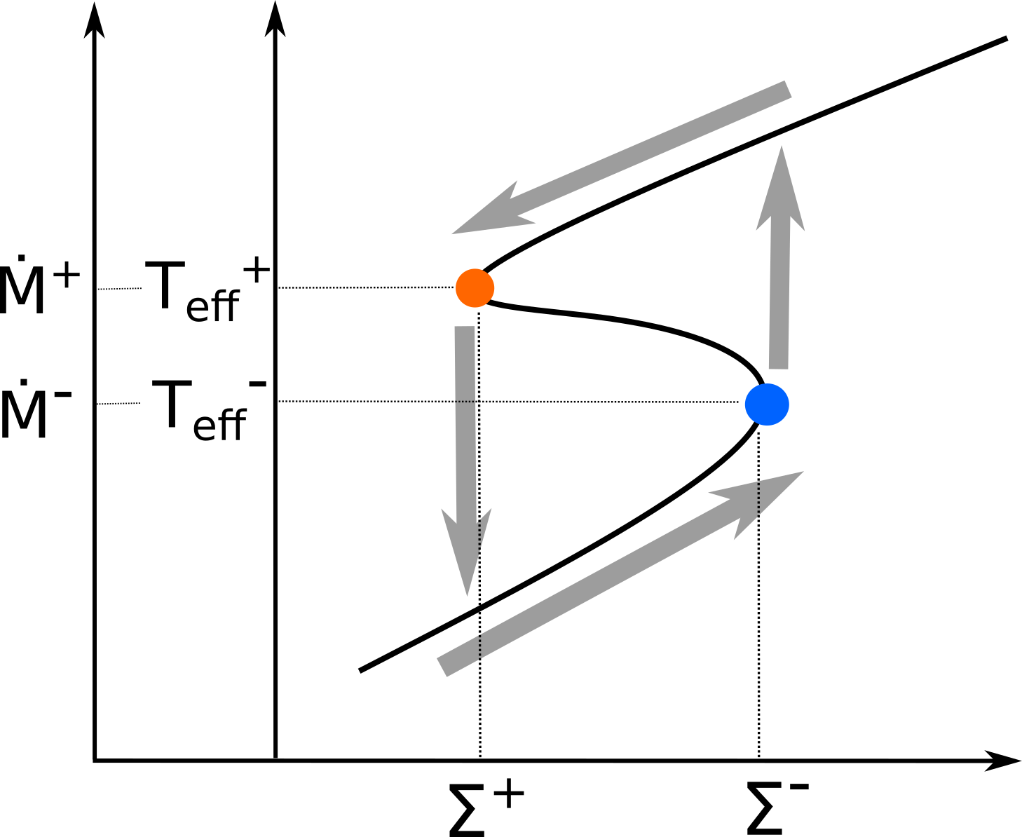
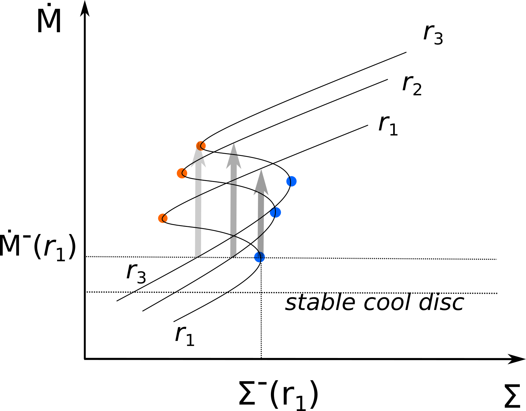
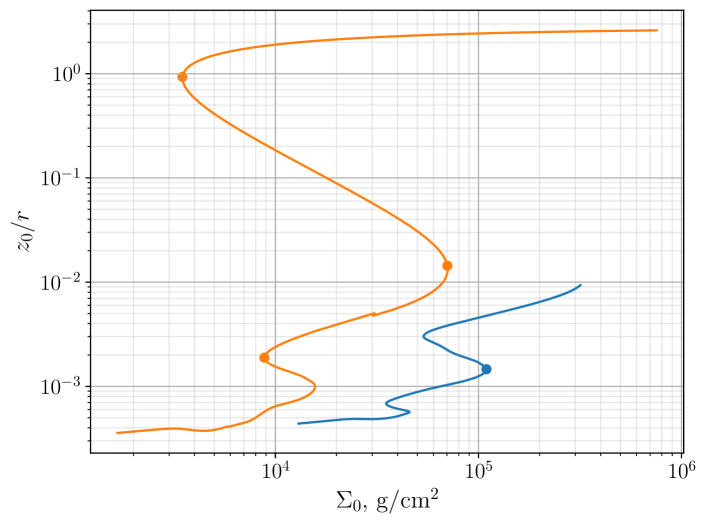
The outburst mechanism can be suitably illustrated using the relationship between the effective temperature or the accretion rate and the surface density (the disc-thickness-integrated bulk density), – S-curve, see, e.g., Fig. 1 or figure 4 in the review by Lasota (2016) (also Meyer & Meyer-Hofmeister, 1981; Smak, 1984b). The S-curves are obtained by solving the disc equations in -direction (vertical structure equations). If the parameters of a particular ring in a disc fall on the negative branch of the S-curve, the ring is in an unstable state. The ionisation instability that drives the DIM occurs at temperatures K.
For example, in low-mass X-ray binaries, matter from a normal star may accumulate in a slowly expanding torus around a compact object. As the mass accumulates, the temperature gradually rises and ionisation of the hydrogen eventually becomes possible. Then a notorious opacity dependence on temperature allows a thermal instability (see e.g. Faulkner et al., 1983). The disc matter becomes hotter and ionised, the viscous time shortens and a mass redistribution leads to the enhanced accretion on the central object and to the electromagnetic flare.
At higher temperatures, the radiation-dominated regime comprises another negative branch of the dependence for larger accretion rates, close to the Eddington limit. This regime is thermally and viscously unstable as well (Lightman & Eardley, 1974; Shakura & Sunyaev, 1976; Piran, 1978). A hotter positive-slope branch emerges at even higher accretion rates when photon trapping with the radially moving matter (advection) acts as an energy sink at each radius (Abramowicz et al., 1988, 1995; Bjoernsson et al., 1996). A corresponding limit cycle behaviour for black hole discs with accretion rates close to Eddington has been proposed (Janiuk & Czerny, 2011; Czerny, 2019, and references therein).
In the present work we study the stability curves for discs around SMBHs in a wide range of accretion rates. These stability curves resemble letter ’’ and have two unstable branches, connected to partial-ionization instability and radiation-pressure instability, and four critical values of the surface density. We find a new scenario of disc heating, triggered by the ionisation instability, which can only occur in a disc around a SMBH and is based on the assumption that the turbulent -parameter becomes higher in ionised discs. The relative positions of the critical points on the stability curve in the case of SMBH allow a disc ring heated by ionisation instability to bypass the gas pressure dominated regime and continue to heat until advection stabilises the disc. This leads to a huge increase in the accretion rate, by a factor of . Such a transition is likely to induce the super-Eddington state, when strong outflows are produced. The large semi-thickness of an optically thick advection-dominated disc explains a comparatively short flare duration.
We expect such flares to be observationally similar to tidal disruption events (TDE), except for the asymmetric manifestations. According to our toy-model estimates, the giant flares can be more powerful and longer than the typical average TDE. Assuming a constant supply of matter from a galaxy to the central SMBH, giant flares may be about ten times less frequent than current observed rate of TDEs. The emission from the initial heating is likely to be in the extreme ultraviolet and optical diapason, followed by soft X-rays, which may be strongly attenuated, as is usually expected from the outflowing accretion discs in the unfortunate geometrical situation.
2 Local stability curves of SMBH discs
Let us first briefly consider an outburst due to thermal-viscous instability using S-curves. We neglect for a while a possible change of the turbulent parameter .
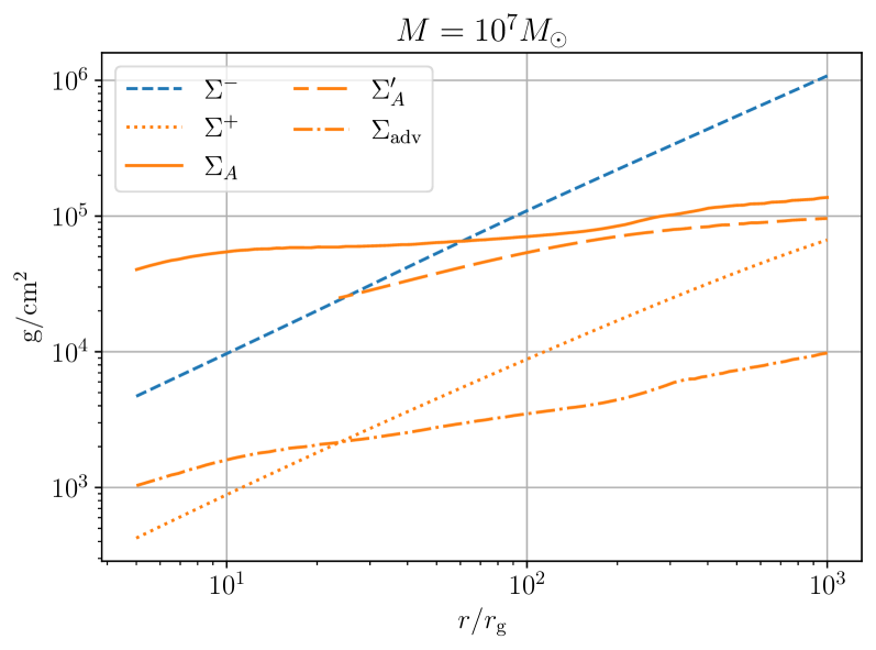
For each radius in a quasi-stationary disc, a proper S-curve can be constructed, see Fig. 2. As we can see, the critical surface densities and at each radius (namely, the abscissas of the turns, – the blue and orange points, – of the S-curve in Fig. 2) bound an interval of the surface density. If the actual of a ring were to lie within this interval, this would mean that the ring would be capable of transitioning to an alternative thermal state (another positive branch) if the thermal equilibrium were disturbed. If the heating is triggered at , the heating wave could reach to but no further, since the disc had the minimum possible density allowing ionization of matter there.
At higher temperatures, an unstable radiation-dominated regime and a stable advective regime of accretion emerge. The analytic relations between the accretion rate and surface density could be obtained for these branches. When the radiation pressure dominates over the gas pressure in the geometrically thin disc (the so-called A-zone, Shakura & Sunyaev, 1973), the height-integrated viscous stress can be expressed algebraically from using the vertical structure equations (Lightman & Eardley, 1974). Here, using the stationary-disc relation between the viscous stress tensor and , we obtain:
| (1) |
where is the turbulent parameter in the disc (Shakura & Sunyaev, 1973), is the angular Keplerian velocity, is the black hole mass, is the Eddington limit
| (2) |
and we adopted -parameters from Tavleev et al. (2023, equation 24), which are dimensionless values obtained by solving or averaging the vertical structure of the disc. 111Omitting the solution of the vertical structure leads to all = 1 as in the approach of Shakura & Sunyaev (1973). The Thomson cross section is denoted by and other symbols have standard meaning.
If the temperature is even higher, for , the central part of the disc becomes geometrically thick (a slim disc) and the radial advection starts to play role. Below we use the definition for the Eddington accretion rate:
| (3) |
Combining the equations for hydrostatic balance and viscous energy release (e.g., Tavleev et al., 2023, equations 1 and 2), or using again the -parameters, we obtain:
| (4) |
The half thickness should satisfy the energy balance equation, which can be solved together with the radial structure of an advective supercritical disc. In the advective regime the disc semi-thickness saturates and we can roughly assume (e.g., Lipunova, 1999; Lasota et al., 2016). The slope of the relation is positive for constant , implying the viscous stability of the advective zone (see Kato et al., 2008).
2.1 Non-stationary discs around SMBH
It has been proposed that in stellar mass systems, the turbulence parameter is higher in ionised material discs compared to neutral matter discs (e.g., Smak, 1984a; Meyer & Meyer-Hofmeister, 2015). We assume different for a cold neutral and a hot fully ionised disc, although the decreasing in the recombined material in AGN discs has been criticised (Menou & Quataert, 2001b). Janiuk et al. (2004) studied the magnetic Reynolds and ambipolar diffusion numbers and found that they appear to exceed the critical values required for sustained turbulence unless the accretion rate is very low. We can speculate that might still depend on the degree of ionisation, as shown for protoplanetary discs by Landry et al. (2013); see also discussion in §2.1 of Hameury et al. (2009).
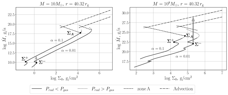
Examples of stability curves for a stellar-mass black hole and a SMBH are shown in Fig. 3. To calculate S-curves for states of the optically-thick and geometrically thin disc around SMBHs, we use our publicly available code (Tavleev et al., 2023). The upper branches are depicted according to Eqs. (1) and (4), by dashed and dot-dashed lines, respectively.
The difference between the S-curves of the stellar-mass BH and the SMBH is easy to see. For a very massive central black hole, the maximum critical surface density in the cold disc around the SMBHfor lower is larger than the maximum critical density of the geometrically thin hot ionised disc for larger .
This can lead to a ‘giant flare’ event. If the surface density in the cold state of a SMBH disc exceeds a critical maximum value the heating instability can lead to a direct transition of the ring to an advective state, skipping a ‘thin ionised’ state. This transition occurs on a thermal timescale. We cannot calculate the course of such heating in this paper. This is generally very difficult to do at the current level of disc simulation. However, the central point of the proposed mechanism is the assumption that if the ring in the diagram (, ) turns out to be at such a large surface density that there is a stable solution only at high temperature, then the ring should transfer to this hot state if it does not lose its density faster. This is similar to the classic mechanism in the DIM model.
An important caveat here is that Figure 3 is constructed for a quasi-stationary disc. Firstly, a quasi-stationary viscous radial torque distribution is assumed. Secondly, a sufficient time must elapse before the disc ‘settles’ and a state on the S-curve can be realised. In the case of a geometrically thin disc, this time must be of the order of the thermal time. In the case of a slim advective disc, whose energy balance is not local, this time can be longer, apparently, of order of the viscous time. This follows from the fact that the quasi-stationary accretion state at the highest positive branch can be achieved only when the radial transfer of energy is established. For the latter, the disc zone in question has to be already thick and advective. However, because the slim disc is quite thick, the viscous time scale is not much longer than the thermal time .
We assume that on the local viscous time scale the slim disc at each radius approaches a state corresponding to a point on the uppermost brunch on the S-curve. The heating may be accompanied with an optical flare of a modest magnitude. At the same time, the accretion rate on the central BH starts to increase and its maximum depends on the mass available in the heated state, i.e. on the range of radii where the disc has switched to the advective state.
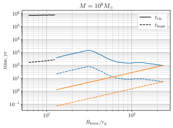
The evolution of the accretion rate on the SMBH depends on how the size of the advective zone decreases with time and on the outflows from the disc surface. The duration of the flares can be estimated as the viscous time at the maximum radius of the advective zone:
| (5) |
This time can be an order or two longer than the orbital time because and few. If one approximates a light curve by the exponential law, the -folding decay time is as follows:
| (6) |
see Appendix A, where
| (7) |
This time is much shorter than the viscous evolution time in the geometrically thin disc around the SMBH due to the fact that in the advective regime and for a thin disc.
In the following section, we abandon the analytical approximations for the branches of the -curves and calculate them numerically. We continue to call them S-curves (stability-curves).
2.2 Turning points of the stability curves
The critical values of the stability curves affect the possibility of a giant flare and its amplitude. To find these values,
| (8) | ||||
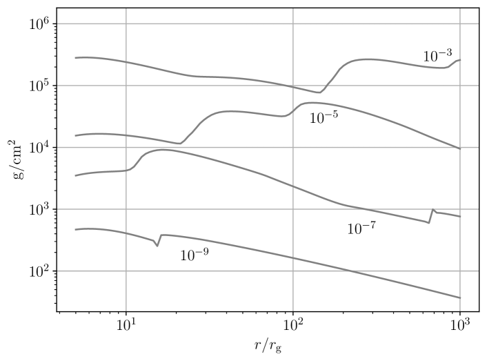
we construct a set of S-curves (see example in Fig. 4(a)) for different SMBH masses.
The S-curves for regimes when the gas pressure dominates are calculated using the open code DiscVerSt by Tavleev et al. (2023). In the radiation-pressure dominated regime, the code of Lipunova (1999) is used, applying a conservative scheme, i.e. without wind. While the super-Eddington accretion disc is expected to launch powerful winds, the critical values of the turning points are not significantly affected by this. The wind has been proposed to start when the total bolometric luminosity of the disc exceeds the Eddington value, shown on the right vertical axis in Fig. 4(a), i.e. on the upper positive branch. The code by Lipunova (1999) calculates the radial structure of a disc with the optional advection-dominated super-Eddington central zone, assuming the constant dimensionless parameters , characterizing the vertical structure (Ketsaris & Shakura, 1998; Tavleev et al., 2023). We stitch the radial structure obtained in the two codes at a point in the interval between and (marked as ‘Hot disc’), using the -values calculated in the DiscVerSt code at this point. To construct the global S-curves (like shown in Figs. 4), we calculate the radial structure for many values of .
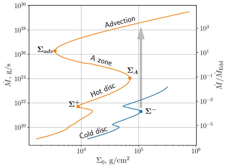
Resulting dependencies of the critical values (8) are shown for one SMBH mass in Fig. 5. Only one curve is calculated with , and others, with . A giant flare can happen if .
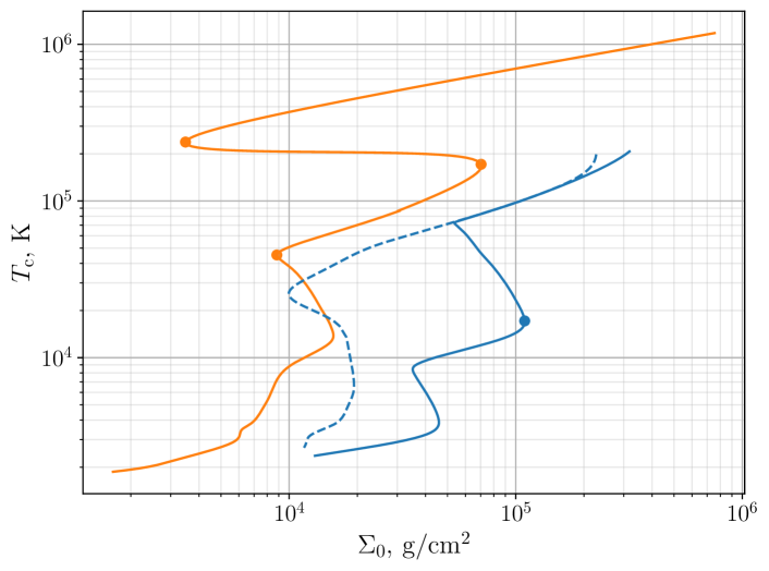
In Fig. 4(b) we also show the stability for a disc calculated without convection by the dashed line. Cannizzo & Reiff (1992) noted that ignoring convection reduces the critical surface density. Our values of agree well with the results of Hameury et al. (2009) with convection.
The semi-thickness of the advective disc is greater than 1 in Fig. 4(c). This can be attributed to the approximate character of the vertical structure approach in the code based on that of (Lipunova, 1999) (in the original paper , which decreases the thickness). Here we keep constant ( few) along the upper S-curve as we are most interested in calculating . In the following analysis, see §4, we assume a value of for the thickness of the advective slim disc.
In Fig. 5, the turning points corresponding to change between the gas- and radiation-pressure-dominated accretion regime are presented as obtained in two alternative ways ( and ). Generally, the vertical structure code DiscVerSt (which includes convection and tabular opacities and calculates values) has numerical difficulties when the radiation pressure is large, but in some cases we have managed to obtain the turning points . We see that at those radii, when we have , – result of DiscVerSt, – it is less than and, thus, cannot hinder the proposed mechanism. For further analysis we will use the dependence, keeping in mind its approximate character.
2.3 Thermal-viscous instability in the disc around SMBH
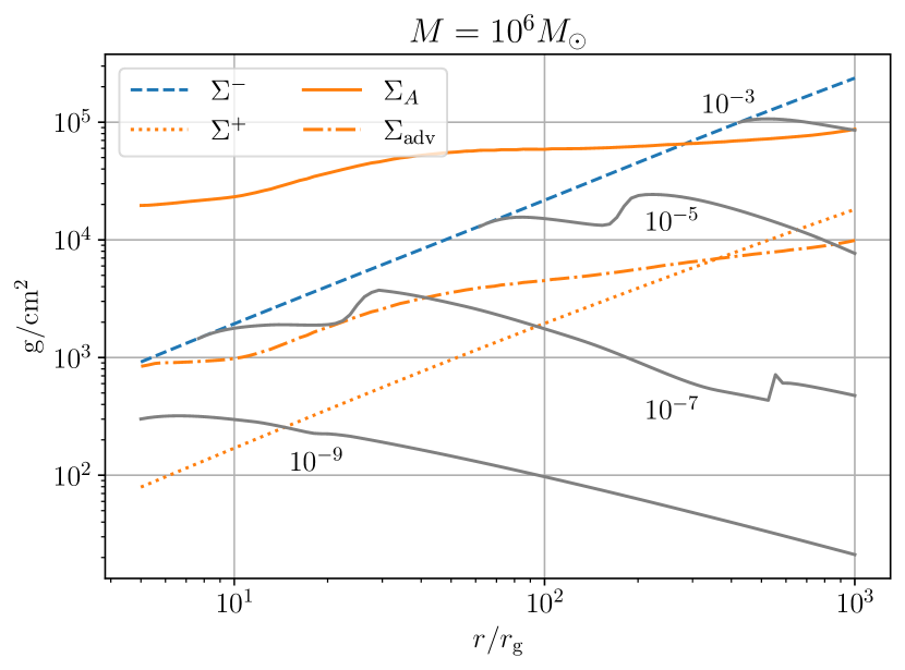
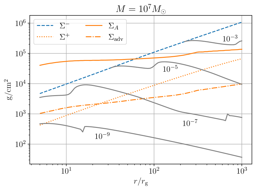
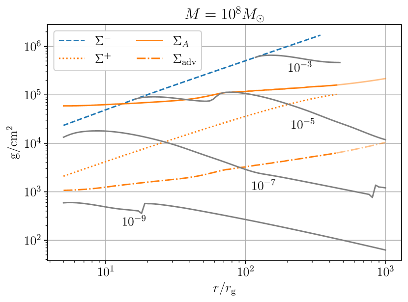
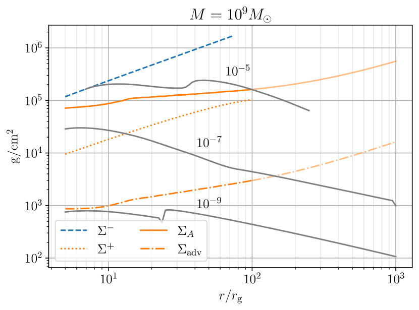
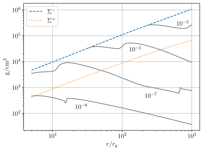
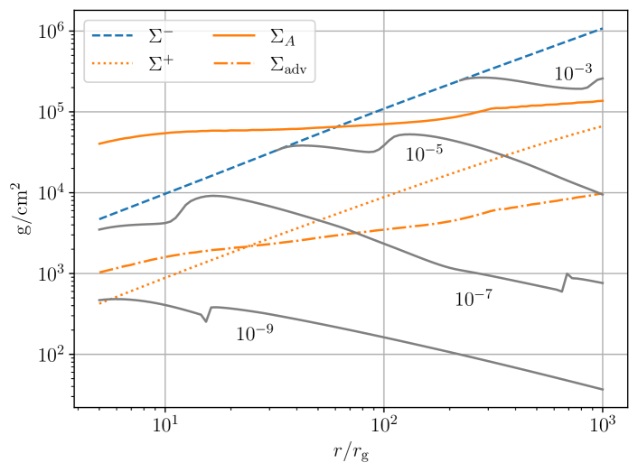
Consider the case of BH with . In Fig. 6a, we show the surface density distributions for several values of accretion rate in a quasi-stationary disc around the SMBH. In the panels (b) and (c), we cut the surface density distributions at the intersections with . The radial dependencies of the critical values of S-curves are plotted too. The similar plots for other SMBH masses can be found in Fig. 14.
In the quiescent epoch, as the mass accumulates in the disc due to income of the galactic matter, in its innermost parts (shown in Fig. 6a) the accretion rate can slowly increase. We imagine that the grey curves change successively in time, replacing each other in order from bottom to top. In reality, the accretion rate probably increases with radius in a quiescent disc. Consequently, realistic would have more positive slope (compare, for example with figure 5b in Hameury et al. 1998). This observation does not lead to qualitative changes in the picture. It can be kept in mind, though, that the accretion rates, indicated in Fig. 6, correspond to the accretion rate at the inner disc radius.
As long as , the whole disc is in the stable cold state (this accretion rate roughly corresponds to the intersection of with a grey curve at the inner disc edge). Nowhere in the disc does the surface density and temperature reach values where hydrogen ionisation triggers the instability.
When the quasi-stationary accretion rate exceeds , the surface density becomes greater than near the inner edge of the disc (see Fig. 6b) . At this radius , see Fig. 6c. This means that the outburst can occur in the classical framework of the DIM model. There will be a transition from the lower cool branch to the upper hot branch near the inner edge of the disc ( is between and ), and the hot front will start to propagate outwards. A rebrightening of the disc also occurs. The accretion rate to the SMBH increases, resulting in a slow outburst with the characteristic time yr, found from (5) by substituting (cf. Fig. 4(c)) and . (Value can be very roughly estimated as the intersection of the grey curve for and the curve , see Fig. 6b).
At the end of the outburst, as the cooling front moves towards the disc centre and the disc surface density falls below , the disc moves to the lower cold branch of the stability curves at each radius. The transition to the lower stable branch is actually possible for any in the interval from to . In that respect the left arrow in Fig. 1 is drawn very tentatively. Due to the external influx of matter, the process can start anew. The time between these flares corresponds to a long viscous time in a geometrically thin cold disc with .
3 Conditions for a ‘giant’ flare
It is believed that to explain the spectral features, evolution and timing of low accretion rate black hole (SMBH and stellar mass) accretion discs, it is necessary to assume that a geometrically thin disc is truncated from the inside and its inner part is replaced by a high temperature and low density accretion flow (see, e.g., Yuan & Narayan, 2014; Nemmen et al., 2014).
The absence of a standard disc at small radii means that, compared to the situation considered in §2.3, the quiescent accretion rate can increase to higher values without the disc triggering an instability. This is due to the fact that the surface density in the central region is lower than in the standard disc (while the radial velocity is higher).
For example, consider a disc around black hole with the truncation radius . As can be seen from Fig. 6b, the quiescent accretion rate must exceed for an outburst similar to the one described in §2.3 to occur: the ring transfers to ‘Hot disc’ state. In particular, if is close enough to , the increased accretion rate from this ring inwards will be such that the inner part of the disc, at , will be in the radiation-pressure instability zone (A zone), potentially driving fluctuations proposed to explain Changing-Look AGN (e.g., Śniegowska et al., 2023).
However, consider a situation where the truncation radius is larger, so large that a giant flare is produced. For this happens when . This value is determined by the intersection of the curves and , see panel (c) in Fig. 6.
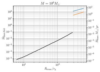
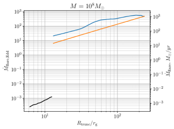
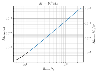
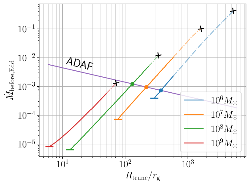
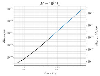
The truncation radius directly determines the accretion rate before a giant flare, which is the critical value of the accretion rate at the turning point (point in Fig. 4(a)). Figure 7 shows the accretion rate before the flare versus the truncation radius for different SMBH masses. We plot the dependencies only for those truncation radii that are larger than the minimum that allows a giant flare to occur. When the truncation radius is smaller than shown in Fig. 7, the thermal instability results in a ‘normal’ outburst and does not heat the disc to the super-Eddington regime. The maximum value of is determined by the self-gravity limit (see Eq. (10) below).
We can compare the truncation radii with those proposed by models such as the Advection-Dominated Accretion Flow (ADAF; Narayan & Yi, 1994) as a replacement for the central standard disc (Narayan, 1996; Esin et al., 1997; Poutanen et al., 1997; Dubus et al., 2001; Menou & Quataert, 2001a; Janiuk et al., 2004; Hameury et al., 2007; Narayan & McClintock, 2008).
To find the transition radius, one needs to consider the physical situation leading to the formation and thermal structure of the transition region(see e.g. Yuan & Narayan, 2014, §4.2.2.). Czerny et al. (2004) examined the data from the Broad Line Regions using optical/UV spectra from the Large Bright Quasar Survey and found evidence for a ‘strong ADAF principle’: the standard geometrically thin solution is chosen by the disc only if it is the only solution available for certain . Accordingly, an estimate of the radius of the boundary between the ADAF and the standard disc (Abramowicz et al. 1995,Czerny et al. 2004; see further references in Sniegowska et al. 2020) is as follows:
| (9) |
Inverted relation (9) is shown in Fig. 7. Taking the purple ‘ADAF’ line in Fig. 7 as an upper bound, we infer that there is potentially a wide range of parameters that allow giant flares to occur. Obviously, the required accretion rates and depend on the ratio ; they grow as the ratio decreases.
4 Properties of the giant flares
Similar to the DIM scenario, the ring heated by the instability can trigger a transition wave (a heating wave) that moves outwards. How far out can such a wave travel? The maximum possible distance is determined by the condition that there (before the outburst) should not be less than (see Fig. 4(a)). This can be difficult to achieve in a ‘rapidly changing landscape’ because, for example, viscous evolution occurs on almost the thermal timescale. We suggest that the minimum extent of the heating wave is on the order of , assuming isotropic heat diffusion.
At a certain radius in the disc, the effects of self-gravity begin to take effect. The distance beyond which the razor-thin disc becomes gravitationally unstable is defined by the following condition (Safronov, 1960; Toomre, 1964):
| (10) |
The behaviour of the disc and beyond depend on the cooling and heating mechanisms there. Given the uncertainties in the disc structure, which are beyond the scope of the present work, we choose to present the results only for radii less than . Also, due to numerical difficulties, we have not calculated flare parameters for very close to , nor have we considered radii larger than , as our primary focus is on lower estimates. The radii we considered are indicated by the solid intervals of the curves in Fig. 7.
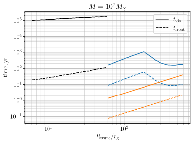
The time before the flare peaks can be estimated as the heating front propagation time (Meyer, 1984):
| (11) |
For a slim disc, the front time is of order of (17). It takes time for the inner accretion rate to peak for a disc whose size is growing only viscously, e.g. after a heating wave has already reached its limit. The caveat here is that the two estimates are derived from different approaches.
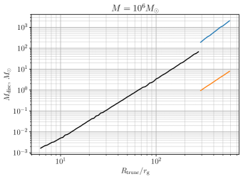
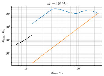
The upper limit of the characteristic flare decay time can be estimated as the viscous time at the outer boundary of the disc involved in the flare , see Eq. (5). The mass of the disc that can participate in the flare:
| (12) |
We neglect here that the surface density changes as the heating front propagates.
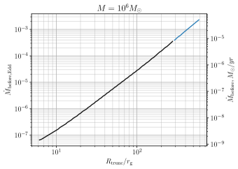
Finally, the peak accretion rate can be approximated as the mass divided by the characteristic time, see Eqs. (18):
| (13) |
It should be remembered that a substantial fraction of the ’heated’ mass is blown away with the outflow. In the slim disc models, the upper limit of the wind loss fraction of the accretion rate has been estimated to be as high as % (Poutanen et al., 2007).
It is evident that the truncation radius determines and before the flare, as well as the power and duration of the flare itself.
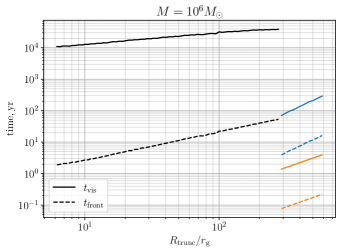
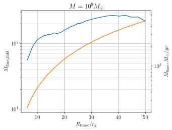
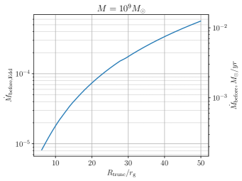
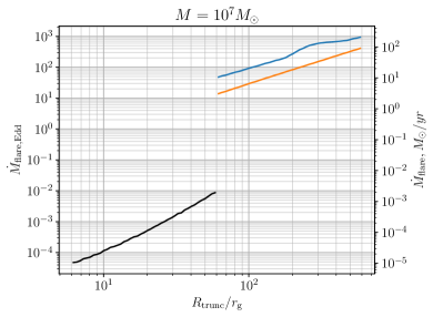
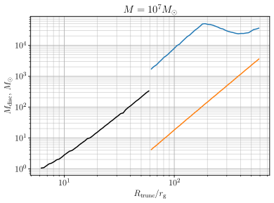
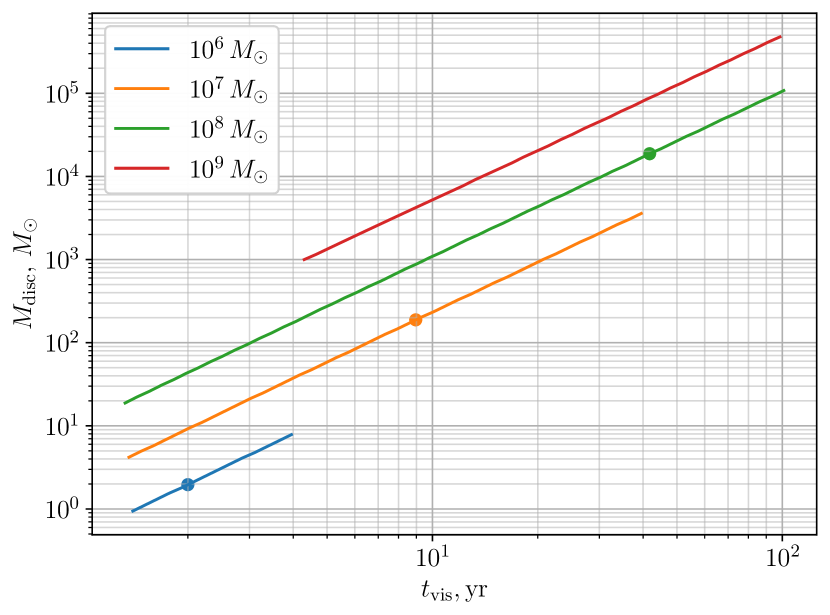
Figures 8 and 11–13 show the calculated parameters of the flares for different SMBH masses: peak accretion rate estimate (13), front time (11) and viscous time (5), accretion rate in a thin disc before the flare, and the mass involved in a flare. The left sets of points (black; absent for ) represent the values calculated for the ‘normal’ under-Eddington flares (see §2.3). The non-monotonic behaviour of the blue curves for is explained by the fact that, according to our assumption, the maximum radius that the heating wave can reach is limited by the radius of the gravitational instability .
Due to the assumed fixed thickness of the slim disc, the ratio between and is about one order everywhere.
For the giant flares, which are faster and more luminous, we plot two sequences: assuming , in blue, and , in orange. For ‘normal’ flares, we use , cf. Fig. 2.
Table 1 is a compilation of the flare characteristics for . This case is the least dependent on the radial distribution of the surface density in the quiescent disc and the most conservative estimate.
The effective temperature of the disc at can be estimated from . Due to the advection effect, we find that the effective temperature can be twice as low; for and , for and , respectively, K.
| 40 | 80 | 200 | – | |
| , yr | ||||
| 2 | 7 | 40 | – | |
| ¿20 | ||||
| 2.5 | 230 | – |
5 Discussion
5.1 Limits of the local analysis
The main shortcoming of the proposed model is that it is based on a local analysis of the S-curves. Numerical simulations show that the trajectories of the parameters of the disc ring during the development of a flare can be quite complicated, even in the case of ”normal” flares, see, e.g., Lasota (2001), figures 11 and 12, Śniegowska et al. (2023), figure 5.
Another possible difficulty is the substantial difference between and required by the mechanism. Overall, this fits well with the modern paradigm (e.g., Martin et al., 2019). Currently, however, there is a lack of confidence in both the magnitude of alpha and its radial constancy. MHD simulations result in varying with the dimensionless disc shear rate (which equals for a Keplerian disc) and due to the potential contribution of large-scale, mean magnetic fields, which can exist near and inside the inner edge of the disc (Penna et al., 2013). In the magnetically supported disc around in the global radiation MHD simulation were obtained (Jiang et al., 2019).
Observational constraints for in the case of AGN were obtained assuming thermal time-scale of the underlying variations’ mechanism. On studyng the UV/optical spectrum variability of 26 AGN Siemiginowska & Czerny (1989) obtained and for 49 AGN Starling et al. (2004) obtained , with . Xie et al. (2009) analysed temporal distance between optical light curve maxima of 31 gamma-ray loud blazars with and got . An analysis of -band light curves as of the continuous time stochastic process for 100 quasars provided a lower (Kelly et al., 2009). The stochastic variability in optical and UV is found to be consistent with in 67 AGN (Burke et al., 2021).
5.2 Giant flares and Tidal Disruption Events (TDE)
TDEs are invoked to explain bright X-ray, UV and/or optical events in galactic centres lasting months to years (Hills, 1975; Rees, 1988). If a star passes close enough to an SMBH, and if the tidal forces exerted by the massive object are strong enough, the star can be ripped apart. After returning to the circularisation radius, which is estimated to be twice the tidal radius ,
| (14) |
some debris is thought to form a viscously evolving disc (Cannizzo et al., 1990; Ulmer, 1999; Shen & Matzner, 2014). The disc of stellar debris, as well as the collisional shock, heats up and emits in a wide range of wavelengths, from optical to X-ray. This sudden increase in brightness is one of the key features used to identify a TDE.
The giant flares involve accretion in the super-Eddington regime, which makes their manifestation similar to that of TDEs (e.g., Shen & Matzner, 2014; Komossa, 2015; Metzger & Stone, 2016; Dai et al., 2018). Similarly, the bolometric luminosity is determined by the disc luminosity, which logarithmically exceeds , plus the emission from the pressure-supported envelope (Sarin & Metzger, 2024). The expected wind velocity is also of order of the escape velocity . As TDEs, giant flares from disc instability can be sources of ultra high-energy cosmic rays (Farrar & Gruzinov, 2009).
Most of the TDE observables come from an advanced stage, when the disc is already formed. Accordingly, in many cases, the reason for the super-Eddington mass accretion cannot be definitively established.
In general, the viscous time of giant flares, as shown in Table 1, is not less than one year, which contrasts with the typical duration of most TDEs. However, care should be taken when defining the times for comparison: Eq. (6) shows that the e-folding time of a flare is about 0.4 times less than and the rise time is about , see Eqs. (11). It should be noted that longer TDEs sometimes occur (Kankare et al., 2017; Lin et al., 2017; He et al., 2021; Yan & Xie, 2018; Zhang, 2023; Bandopadhyay et al., 2024). At this stage, we do not want to regard our flare parameters as restrictive, since they are derived from the simplest estimates of the viscous disc evolution model. The parameters given in Table 1 are physically the upper limits for actual giant flares, taking into account that (1) accretion discs with a shrinking outer boundary evolve faster than those with a fixed outer boundary, (2) outflows from radii comparable to the outer disc radius accelerate the evolution 222For , at the slim advective disc cannot exist at (see Fig. 4(a)). This shows that the zone of , which is the ‘short viscous time zone’, is shrinking. In this sense, the solution for an expanding disc from Cannizzo et al. (1990) is not applicable..
Spectral line shapes of TDE are used to extract geometry and kinematics of the photoionised gas. In some works, the interpretation due to the expanding spherical outflow is favoured without invoking the typical prescription of an elliptical disc. (Hung et al., 2019). Kara et al. (2018) found an indication of a ionised outflow in ASASSN-14li at early times (about first 40 days), consistent with the O VIII absorption. Using the ionization parameter , the upper limit on the outflow rate can be obtained: /yr. Matsumoto & Piran (2021) applied the ‘reprocessing-outflow’ model for the optically-thick quasi-spherical wind. By considering observed luminosity, temperature, and outflow velocity, they arrived at the conclusion that the outflows are excessively massive: approximately one order of magnitude more mass than what is available in a TDE scenario ().
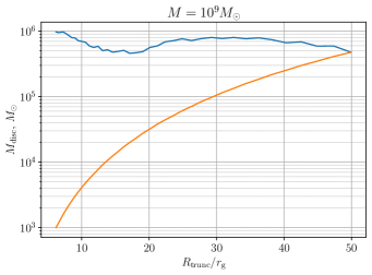
A giant flare scenario could help to resolve this issue. In the last panel of Fig. 8 and Fig. 11–13 we show estimates (12) of the excited mass: they are comparable to or much larger than the typical stellar masses, see also Table 1. Fig. 9 shows the corresponding result for the most modest giant flares, obtained with a rough minimum estimate of the heated zone of the disc, .
At the same time, in several instances, there are observations strongly suggesting that a TDE event preceded the outburst. For example, spectroscopic observations of AT 2020zso indicate the elliptical geometry of the emitter (Wevers et al., 2022), while the authors cite several previous works where emission from quasi-circular discs was reported. Further, event AT 2019azh shows signatures of both the stream-stream collision and delayed accretion (Liu et al., 2022). Linearly polarised optical emission at the level of observed from AT 2020mot possibly indicate accretion disc formation, when ‘the stream of stellar material collides with itself’ (Liodakis et al., 2023).
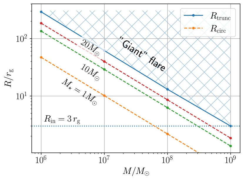
Figure 10 depicts the minimum truncation radius necessary for the ionization instability to trigger a giant flare versus SMBH mass. Notably, for SMBH with , any outburst in a disc with and will be a giant flare, provided the geometrically-thin accretion disc exists at the accretion rates less than . We also plot for stars of different masses, where dependence for the main sequence stars was used (Kippenhahn et al., 2012). It can be seen that a tidal disruption of a massive enough star can ignite a giant flare in a disc, which will increase the TDE output. This happens because the fallback material presumably forms a disc. For example, in the simulations by Andalman et al. (2022), the fallback following the complete destruction of a star near a SMBH results in a disc up to .
5.3 Dew cycle
The process of supplying mass to the central galactic discs during quiescent periods remains unclear (Lodato, 2012; Alexander & Hickox, 2012). At distances of pc in the disc, the self-gravity effects such as spiral waves, fragmentation, and subsequent star formation are possible. The influence of these effects on the mass increase in the central cold disc is quite complex, as they can both nourish and hinder the feeding of SMBHs (Nayakshin et al., 2007; Hopkins & Quataert, 2010). Other possible ways of feeding the central black hole have also been proposed, for example by the very low angular momentum gas (King & Pringle, 2006).
Candidates for galaxies capable of producing giant flares include low-luminosity AGN (LLAGN) (Yuan & Narayan, 2014) and other quiescent SMBHs (Soria et al., 2006; Volonteri et al., 2011) if a geometrically thin accretion disc manages to form at . For very massive SMBH, the development of giant flares may be impossible due to the absence of a cold molecular disc, because the radius of the gravitational instability decreases with the increasing mass. For , the radius of the self-gravity instability is less than the assumed ADAF boundary (see Fig. 7).
For low-mass stellar X-ray binaries, it is common to assume that a binary is transient, i.e. it experiences outbursts, if the transfer rate from a neighbouring star through the Lagrangian point is between and . The ratio between these values is only in Fig. 2. Does this mean that only galaxies with such a rate of mass supply can have giant flares? Obviously not, since galaxies in the process of increasing their central accretion rate from very low levels could also be susceptible to giant flares.
Assuming a constant mass supply from the distant reservoir to the cold disc, the upper limit on the time between giant flares can be considered as the time required for the viscous flow in the geometrically thin disc to reach the inner radii and grow to a critical value. For the sake of estimation and order of magnitude, this can be approximated by the analytical peak time of an outburst (see Appendix A) which gives , where we have substituted , . The radius corresponds to the extent of the mass reservoir, which appears to be larger than , but possibly only by a factor of a few to 10. If a giant flare does not reach a certain radius of the disc, this means that the mass reservoir there is intact. Consequently, the lower the estimates of the flare amplitude, the shorter the replenishment times.
However, taking into account the possibility of very complex matter supply pathways, this estimate may be far from the actual replenishment time. Note that possible events of tidal stripping of stars (‘partial TDE’, see Chen & Shen, 2021) can significantly reduce the time between giant flares.
Given that the rate of ‘complete’ TDEs is estimated to be 1 event per yr, see van Velzen et al. (2020); Saxton et al. (2021) and references therein, Sazonov et al. (2021); Masterson et al. (2024), we suggest that giant flares, if the mechanism is confirmed, could contribute to the observed TDE rate.
6 Summary
We propose a novel mechanism for outbursts associated with the ionisation-viscous instability in the accretion disc. According to our proposal, a massive, cold, neutral, geometrically thin disc with vertical convective energy transfer can transition to a slim, advection-dominated regime within a few thermal timescales, provided that the critical surface density is accumulated. The mechanism is only viable in discs around SMBH and if the turbulent parameter grows in the ionised disc.
For example, if and , and the SMBH mass is , the giant flare can develop if the geometrically thin accretion disc exists at accretion rates less than . Also, any flare due to ionization instability in a geometrically thin convective neutral disc around SMBH with will be a giant flare.
For lighter SMBH, a giant outburst can develop if there is a geometrically thin accretion disc and its inner part is truncated by an optically thin, tenuous flow. An ADAF is a compelling candidate for such a scenario.
Estimated peak accretion rates depend on the size of the disc region transitioning to the ionised state and are , but may be somewhat reduced by the strong outflows. The characteristic outburst duration is estimated by the viscous time of a slim disc, which also depends on the size of the region involved in a flare and can range from several months to several years.
The present calculations should be considered as a rough estimate. The possibility of giant flare development needs to be further investigated using numerical models that can account for non-equilibrium processes in accretion discs.
If confirmed, giant flares could contribute to a variety of bright extragalactic phenomena, such as TDE.
References
- Abramowicz et al. (1995) Abramowicz, M. A., Chen, X., Kato, S., Lasota, J.-P., & Regev, O. 1995, ApJ, 438, L37
- Abramowicz et al. (1988) Abramowicz, M. A., Czerny, B., Lasota, J. P., & Szuszkiewicz, E. 1988, ApJ, 332, 646
- Alexander & Hickox (2012) Alexander, D. M. & Hickox, R. C. 2012, New A Rev., 56, 93
- Andalman et al. (2022) Andalman, Z. L., Liska, M. T. P., Tchekhovskoy, A., Coughlin, E. R., & Stone, N. 2022, MNRAS, 510, 1627
- Bandopadhyay et al. (2024) Bandopadhyay, A., Fancher, J., Athian, A., et al. 2024, ApJ, 961, L2
- Bjoernsson et al. (1996) Bjoernsson, G., Abramowicz, M. A., Chen, X., & Lasota, J.-P. 1996, ApJ, 467, 99
- Burke et al. (2021) Burke, C. J., Shen, Y., Blaes, O., et al. 2021, Science, 373, 789
- Cannizzo et al. (1990) Cannizzo, J. K., Lee, H. M., & Goodman, J. 1990, ApJ, 351, 38
- Cannizzo & Reiff (1992) Cannizzo, J. K. & Reiff, C. M. 1992, ApJ, 385, 87
- Chen & Shen (2021) Chen, J.-H. & Shen, R.-F. 2021, ApJ, 914, 69
- Czerny (2019) Czerny, B. 2019, Universe, 5, 131
- Czerny et al. (2004) Czerny, B., Rózańska, A., & Kuraszkiewicz, J. 2004, A&A, 428, 39
- Dai et al. (2018) Dai, L., McKinney, J. C., Roth, N., Ramirez-Ruiz, E., & Miller, M. C. 2018, ApJ, 859, L20
- Dubus et al. (2001) Dubus, G., Hameury, J. M., & Lasota, J. P. 2001, A&A, 373, 251
- Esin et al. (1997) Esin, A. A., McClintock, J. E., & Narayan, R. 1997, ApJ, 489, 865
- Farrar & Gruzinov (2009) Farrar, G. R. & Gruzinov, A. 2009, ApJ, 693, 329
- Faulkner et al. (1983) Faulkner, J., Lin, D. N. C., & Papaloizou, J. 1983, MNRAS, 205, 359
- Hameury (2020) Hameury, J. M. 2020, Advances in Space Research, 66, 1004
- Hameury et al. (2007) Hameury, J.-M., Lasota, J.-P., & Viallet, M. 2007, in Black Holes from Stars to Galaxies – Across the Range of Masses, ed. V. Karas & G. Matt, Vol. 238, 297–300
- Hameury et al. (1998) Hameury, J.-M., Menou, K., Dubus, G., et al. 1998, MNRAS, 298, 1048
- Hameury et al. (2009) Hameury, J. M., Viallet, M., & Lasota, J. P. 2009, A&A, 496, 413
- He et al. (2021) He, J. S., Dou, L. M., Ai, Y. L., et al. 2021, A&A, 652, A15
- Hills (1975) Hills, J. G. 1975, Nature, 254, 295
- Hopkins & Quataert (2010) Hopkins, P. F. & Quataert, E. 2010, MNRAS, 407, 1529
- Hung et al. (2019) Hung, T., Cenko, S. B., Roth, N., et al. 2019, ApJ, 879, 119
- Janiuk & Czerny (2011) Janiuk, A. & Czerny, B. 2011, MNRAS, 414, 2186
- Janiuk et al. (2004) Janiuk, A., Czerny, B., Siemiginowska, A., & Szczerba, R. 2004, ApJ, 602, 595
- Jiang et al. (2019) Jiang, Y.-F., Blaes, O., Stone, J. M., & Davis, S. W. 2019, ApJ, 885, 144
- Kankare et al. (2017) Kankare, E., Kotak, R., Mattila, S., et al. 2017, Nature Astronomy, 1, 865
- Kara et al. (2018) Kara, E., Dai, L., Reynolds, C. S., & Kallman, T. 2018, MNRAS, 474, 3593
- Kato et al. (2008) Kato, S., Fukue, J., & Mineshige, S. 2008, Black-Hole Accretion Disks — Towards a New Paradigm —
- Kelly et al. (2009) Kelly, B. C., Bechtold, J., & Siemiginowska, A. 2009, ApJ, 698, 895
- Ketsaris & Shakura (1998) Ketsaris, N. A. & Shakura, N. I. 1998, Astronomical and Astrophysical Transactions, 15, 193
- King & Pringle (2006) King, A. R. & Pringle, J. E. 2006, MNRAS, 373, L90
- Kippenhahn et al. (2012) Kippenhahn, R., Weigert, A., & Weiss, A. 2012, Stellar Structure and Evolution
- Komossa (2015) Komossa, S. 2015, Journal of High Energy Astrophysics, 7, 148
- Landry et al. (2013) Landry, R., Dodson-Robinson, S. E., Turner, N. J., & Abram, G. 2013, ApJ, 771, 80
- Lasota (2001) Lasota, J.-P. 2001, New A Rev., 45, 449
- Lasota (2016) Lasota, J.-P. 2016, in Astrophysics and Space Science Library, Vol. 440, Astrophysics of Black Holes: From Fundamental Aspects to Latest Developments, ed. C. Bambi, 1
- Lasota et al. (2016) Lasota, J. P., Vieira, R. S. S., Sadowski, A., Narayan, R., & Abramowicz, M. A. 2016, A&A, 587, A13
- Lightman & Eardley (1974) Lightman, A. P. & Eardley, D. M. 1974, ApJ, 187, L1
- Lin et al. (2017) Lin, D., Guillochon, J., Komossa, S., et al. 2017, Nature Astronomy, 1, 0033
- Liodakis et al. (2023) Liodakis, I., Koljonen, K. I. I., Blinov, D., et al. 2023, Science, 380, 656
- Lipunova (1999) Lipunova, G. V. 1999, Astronomy Letters, 25, 508
- Lipunova (2015) Lipunova, G. V. 2015, ApJ, 804, 87
- Liu et al. (2022) Liu, X.-L., Dou, L.-M., Chen, J.-H., & Shen, R.-F. 2022, ApJ, 925, 67
- Lodato (2012) Lodato, G. 2012, Advances in Astronomy, 2012, 846875
- Lynden-Bell & Pringle (1974) Lynden-Bell, D. & Pringle, J. E. 1974, MNRAS, 168, 603
- Martin et al. (2019) Martin, R. G., Nixon, C. J., Pringle, J. E., & Livio, M. 2019, New A, 70, 7
- Masterson et al. (2024) Masterson, M., De, K., Panagiotou, C., et al. 2024, ApJ, 961, 211
- Matsumoto & Piran (2021) Matsumoto, T. & Piran, T. 2021, MNRAS, 502, 3385
- Menou & Quataert (2001a) Menou, K. & Quataert, E. 2001a, ApJ, 562, L137
- Menou & Quataert (2001b) Menou, K. & Quataert, E. 2001b, ApJ, 552, 204
- Metzger & Stone (2016) Metzger, B. D. & Stone, N. C. 2016, MNRAS, 461, 948
- Meyer (1984) Meyer, F. 1984, A&A, 131, 303
- Meyer & Meyer-Hofmeister (1981) Meyer, F. & Meyer-Hofmeister, E. 1981, A&A, 104, L10
- Meyer & Meyer-Hofmeister (2015) Meyer, F. & Meyer-Hofmeister, E. 2015, PASJ, 67, 52
- Mineshige & Shields (1990) Mineshige, S. & Shields, G. A. 1990, ApJ, 351, 47
- Narayan (1996) Narayan, R. 1996, ApJ, 462, 136
- Narayan & McClintock (2008) Narayan, R. & McClintock, J. E. 2008, New A Rev., 51, 733
- Narayan & Yi (1994) Narayan, R. & Yi, I. 1994, ApJ, 428, L13
- Nayakshin et al. (2007) Nayakshin, S., Cuadra, J., & Springel, V. 2007, MNRAS, 379, 21
- Nemmen et al. (2014) Nemmen, R. S., Storchi-Bergmann, T., & Eracleous, M. 2014, MNRAS, 438, 2804
- Penna et al. (2013) Penna, R. F., S\kadowski, A., Kulkarni, A. K., & Narayan, R. 2013, MNRAS, 428, 2255
- Piran (1978) Piran, T. 1978, ApJ, 221, 652
- Poutanen et al. (1997) Poutanen, J., Krolik, J. H., & Ryde, F. 1997, MNRAS, 292, L21
- Poutanen et al. (2007) Poutanen, J., Lipunova, G., Fabrika, S., Butkevich, A. G., & Abolmasov, P. 2007, MNRAS, 377, 1187
- Rees (1988) Rees, M. J. 1988, Nature, 333, 523
- Safronov (1960) Safronov, V. S. 1960, Annales d’Astrophysique, 23, 979
- Sarin & Metzger (2024) Sarin, N. & Metzger, B. D. 2024, ApJ, 961, L19
- Saxton et al. (2021) Saxton, R., Komossa, S., Auchettl, K., & Jonker, P. G. 2021, Space Sci. Rev., 217, 18
- Sazonov et al. (2021) Sazonov, S., Gilfanov, M., Medvedev, P., et al. 2021, MNRAS, 508, 3820
- Shakura et al. (2018) Shakura, N. I., Lipunova, G. V., Malanchev, K. L., et al. 2018, Accretion flows in astrophysics (New York: New York)
- Shakura & Sunyaev (1973) Shakura, N. I. & Sunyaev, R. A. 1973, A&A, 500, 33
- Shakura & Sunyaev (1976) Shakura, N. I. & Sunyaev, R. A. 1976, MNRAS, 175, 613
- Shen & Matzner (2014) Shen, R.-F. & Matzner, C. D. 2014, ApJ, 784, 87
- Siemiginowska & Czerny (1989) Siemiginowska, A. & Czerny, B. 1989, MNRAS, 239, 289
- Siemiginowska et al. (1996) Siemiginowska, A., Czerny, B., & Kostyunin, V. 1996, ApJ, 458, 491
- Smak (1984a) Smak, J. 1984a, Acta Astron., 34, 161
- Smak (1984b) Smak, J. 1984b, PASP, 96, 5
- Sniegowska et al. (2020) Sniegowska, M., Czerny, B., Bon, E., & Bon, N. 2020, A&A, 641, A167
- Śniegowska et al. (2023) Śniegowska, M., Grzȩdzielski, M., Czerny, B., & Janiuk, A. 2023, A&A, 672, A19
- Soria et al. (2006) Soria, R., Graham, A. W., Fabbiano, G., et al. 2006, ApJ, 640, 143
- Starling et al. (2004) Starling, R. L. C., Siemiginowska, A., Uttley, P., & Soria, R. 2004, MNRAS, 347, 67
- Tavleev et al. (2023) Tavleev, A. S., Lipunova, G. V., & Malanchev, K. L. 2023, MNRAS, 524, 3647
- Toomre (1964) Toomre, A. 1964, ApJ, 139, 1217
- Ulmer (1999) Ulmer, A. 1999, ApJ, 514, 180
- van Velzen et al. (2020) van Velzen, S., Holoien, T. W. S., Onori, F., Hung, T., & Arcavi, I. 2020, Space Sci. Rev., 216, 124
- Volonteri et al. (2011) Volonteri, M., Dotti, M., Campbell, D., & Mateo, M. 2011, ApJ, 730, 145
- Wevers et al. (2022) Wevers, T., Nicholl, M., Guolo, M., et al. 2022, A&A, 666, A6
- Xie et al. (2009) Xie, Z. H., Ma, L., Zhang, X., et al. 2009, ApJ, 707, 866
- Yan & Xie (2018) Yan, Z. & Xie, F.-G. 2018, MNRAS, 475, 1190
- Yuan & Narayan (2014) Yuan, F. & Narayan, R. 2014, ARA&A, 52, 529
- Zhang (2023) Zhang, X. 2023, ApJ, 948, 68
Acknowledgements.
We thank Arman Tursunov for comments on the manuscript. We acknowledge the usage of computing resources of the M. V. Lomonosov Moscow State University Program of Development. Support was provided by Schmidt Sciences, LLC. for KM.Appendix A Analytic relations for -folding time and peak accretion rate
Lipunova (2015) shows that the -folding decay time of the accretion rate evolution in a finite disc with constant viscosity 333For spatially confined accretion disc with varying viscosity , evolution is described by a power-law dependence on time but can be approximated by exponential for a limited time interval. is related to the viscous time as follows:
| (15) |
where is the parameter defined by the viscosity type, introduced by Lynden-Bell & Pringle (1974) and depends on the boundary conditions (Lipunova 2015) and lies in the interval for many cases of accreting discs.
The peak accretion rate in the solution of Lynden-Bell & Pringle (1974) for the infinite disc is
| (16) |
with
| (17) |
(see Appendix of Lipunova 2015).
Combining above formulae, we arrive at
| (18) |
with for , appropriate for discs with constant semi-thickness. For such discs, the dimensionless factor in (15) is about 0.4.
Following the vertical structure solution, we employ
| (19) |
and substitute (see Shakura et al. 2018, §1.5.2 and equation 1.148).
Fiures 11–13 show the same flare characteristics as Fig. 8 for other considered masses of SMBH. They are calculated according to the scheme described in §4 and using the critical surface densities, which could be viewed for different masses in Fig. 14.
In Figure 14, for and , the stationary distributions are plotted only for defined by (10). For these SMBH masses, critical cannot be found for large because the positive hot geometrically thin branch of the S-curve disappears. In this case the values and , which require at a point on this brach, are extrapolated from smaller radii. These intervals are shown as transparent in the lower panels of Fig. 14. The extrapolated values affect only the flare caracteristics calculated if .