Numerical Discretization Methods
for Linear Quadratic Control Problems
with Time Delays

Zhanhao Zhang    Steen Hørsholt    John Bagterp Jørgensen Department of Applied Mathematics and Computer Science
Technical University of Denmark, DK-2800 Kgs. Lyngby, Denmark (e-mail: {jbjo}@dtu.dk)
Abstract

This paper presents the numerical discretization methods of the continuous-time linear-quadratic optimal control problems (LQ-OCPs) with time delays. We describe the weight matrices of the LQ-OCPs as differential equations systems, allowing us to derive the discrete equivalent of the continuous-time LQ-OCPs. Three numerical methods are introduced for solving proposed differential equations systems: 1) the ordinary differential equation (ODE) method, 2) the matrix exponential method, and 3) the step-doubling method. We implement a continuous-time model predictive control (CT-MPC) on a simulated cement mill system, and the objective function of the CT-MPC is discretized using the proposed LQ discretization scheme. The closed-loop results indicate that the CT-MPC successfully stabilizes and controls the simulated cement mill system, ensuring the viability and effectiveness of LQ discretization.

keywords:
Linear Quadratic Optimal Control \sepNumerical Discretization \sepTime Delay Systems

, ,

1 Introduction

Time delays are common in many industrial processes, shaping control systems’ trajectories by not solely relying on the present state but also integrating their history. These delays can significantly influence the robustness and control performance (Lee, 1995; Gu et al., 2003).The linear-quadratic optimal control problems (LQ-OCPs) with time delays find extensive practical applications and needs tailored algorithms for the system identification (Jørgensen and Jørgensen, 2007a, c, b) as well as in the linear quadratic Gaussian (LQG) control and model predictive control (MPC) implementation (Jørgensen et al., 2012; Frison and Jørgensen, 2013). Therefore, there is a need for discretization methods tailored for LQ-OCPs with time delays.

Although research on discretization methods for time-delay systems is extensive (Franklin et al., 1990; Kassas and Dunia, 2006; Hendricks et al., 2008; Otto and Radons, 2017), studies on discretization methods for continuous-time LQ-OCP, particularly incorporating with time delays, are limited. Hendricks et al. (2008) introduced the discrete-time approximation for LQ-OCPs without time delays, employing the zero-order hold (ZOH) parameterization on system states and inputs. Åström (1970)Åström and Wittenmark (2011) and Franklin et al. (1990) provided analytical expressions for equivalent discrete weighting matrices by extending continuous-time cost functions, which can be solved using the matrix exponential method (Moler and Van Loan, 1978; Al-Mohy and Higham, 2011). The discretization and solution methods for continuous-time linear-quadratic regulator (CLQR) problems are described by Pannocchia et al. (2010, 2015). They used the matrix exponential method to obtain the discrete equivalent and proposed a novel computational procedure for solving the optimal control problem.

On the other hand, stochastic LQ-OCPs can be valuable in some scenarios, such as Conditional Value-at-Risk (CVaR) optimization problems (Rockafellar and Uryasev, 2001; Capolei et al., 2015). Åström (1970) and Åström and Wittenmark (2011) introduced the analytic expressions of continuous-time stochastic LQ-OCPs’ cost function and described its expectation. However, as far as we know, the existing literature has not addressed the case of time delays or stochastic systems. In this paper, we thus focus on discretization methods for deterministic and stochastic LQ-OCPs with time delays. The key problems that we address in this paper:

  • 1.

    Formulation of differential equation systems for LQ discretization with time delays

  • 2.

    Numerical methods for solving resulting systems of differential equations

This paper is organized as follows. Section 2 introduces the discretization of time-delay systems and deterministic and stochastic LQ-OCPs with time delays. The discrete weighting matrices are described as differential equation systems. Section 3 describes three numerical methods for solving proposed differential equation systems. We test the proposed numerical methods by a numerical experiment in Section 4 and give the conclusions in Section 5.

2 Linear-Quadratic Optimal Control Problems

This section describes deterministic and stochastic LQ-OCPs with time delays.

2.1 Certainty equivalent LQ for deterministic time-delay systems

Consider a SISO, time-delay, linear state space model

$\displaystyle\dot{x}(t)$ $\displaystyle=A_{c}x(t)+B_{c}u(t-\tau),$ (1a)
$\displaystyle z(t)$ $\displaystyle=C_{c}x(t)+D_{c}u(t-\tau),$ (1b)

where $x\in\mathbb{R}^{n_{x}\times 1}$ is the state, $u\in\mathbb{R}^{n_{u}\times 1}$ is the input and $z\in\mathbb{R}^{n_{z}\times 1}$ is the output. $\tau\in\mathbb{R}^{+}_{0}$ is the input time delay.

Assuming piece-wise constant input $u(t)=u_{k}$ for $t_{k}\leq t<t_{k+1}$ and $T_{s}$ is the sampling time. Note that $m\in\mathbb{Z}^{+}_{0}$ and $0\leq v<1$ are the integer and fractional time delay constants for $l=\tau/T_{s}=m-v$. By taking integral on both side, we obtain the solution of (1)

$\displaystyle x(t)$ $\displaystyle=A(t)x_{k}+B_{o}(t)\tilde{u}_{k},$ (2a)
$\displaystyle z(t)$ $\displaystyle=C_{c}x(t)+D_{c}u_{k-m}=C_{c}x(t)+D_{o}\tilde{u}_{k},$ (2b)

where $\tilde{u}_{k}=[u_{o,k};u_{k}]$ is the augmented input vector and $u_{o,k}=[u_{k-m};\cdots;u_{k-1}]$ is the historical input vector.

The corresponding system matrices are

$\displaystyle A(t)=e^{A_{c}t},$ $\displaystyle B_{1}(t)=\int_{0}^{t}A(s)dsB_{1c},$ (3a)
$\displaystyle A_{v}(t)=e^{vA_{c}t},$ $\displaystyle B_{2}(t)=v\int_{0}^{t}A_{v}(s)ds(B_{2c}-B_{1c}),$ (3b)
$\displaystyle B_{1c}=B_{c}e^{1}_{m+1},$ $\displaystyle B_{2c}=B_{c}e^{2}_{m+1},$ (3c)
$\displaystyle D_{o}=D_{c}e^{1}_{m+1},$ $\displaystyle B_{o}(t)=B_{1}(t)+B_{2}(t),$ (3d)

where $e^{p}_{m+1}=[0\cdots I\cdots 0]$ for $p=1,2,\ldots,m+1$ is an unit vector for selecting $u_{k-(m+1)+p}$ from $\tilde{u}_{k}$ such that $u_{k-{m+1}+p}=e^{p}_{m+1}\tilde{u}_{k}$.

Set $t=T_{s}$, and we obtain

$\displaystyle\overbrace{\left[\begin{array}[]{c}x_{k+1}\\ \hdashline[2pt/2pt]u_{o,k+1}\end{array}\right]}^{=\tilde{x}_{k+1}}$ $\displaystyle=\overbrace{\left[\begin{array}[]{c;{2pt/2pt}c}A&B_{o,1}\\ \hdashline[2pt/2pt]0&I_A\end{array}\right]}^{=\tilde{A}}\overbrace{\left[\begin{array}[]{c}x_{k}\\ \hdashline[2pt/2pt]u_{o,k}\end{array}\right]}^{=\tilde{x}_{k}}+\overbrace{\left[\begin{array}[]{c}B_{o,2}\\ \hdashline[2pt/2pt]I_{B}\end{array}\right]}^{=\tilde{B}}u_{k},$ (4i)
$\displaystyle z_{k}$ $\displaystyle=\overbrace{\left[\begin{array}[]{c;{2pt/2pt}c}C_{c}&D_{o,1}\end{array}\right]}^{=\tilde{C}}\tilde{x}_{k}+\overbrace{D_{o,2}}^{=\tilde{D}}u_{k},$ (4k)

where the system matrices are

$\displaystyle B_{o,1}=B_{o}(:,1:end-n_{u}),\,$ $\displaystyle B_{o,2}=B_{o}(:,mn_{u}:end),$ (5a)
$\displaystyle D_{o,1}=D_{o}(:,1:end-n_{u}),$ $\displaystyle D_{o,2}=D_{o}(:,mn_{u}:end),$ (5b)
$\displaystyle I_{A}=\begin{bmatrix}0&I&\ldots&0\\ \vdots&\vdots&\ddots&\vdots\\ 0&0&\ldots&I\\ 0&0&\ldots&0\end{bmatrix},$ $\displaystyle I_{B}=\begin{bmatrix}0\\ \vdots\\ 0\\ I\end{bmatrix}.$ (5c)

To present time delays in one single MIMO state space model, we consider the following $n_{z}\times n_{u}$ SISO systems

$\displaystyle\dot{x}_{ij}(t)$ $\displaystyle=A_{c,ij}x_{ij}(t)+B_{c,ij}u_{j}(t-\tau_{ij}),$ (6a)
$\displaystyle z_{ij}(t)$ $\displaystyle=C_{c,ij}x_{ij}(t)+D_{c,ij}u_{j}(t-\tau_{ij}),$ (6b)
with
$\displaystyle\quad u=[u_{1};u_{2};\ldots,u_{n_{u}}],$ $\displaystyle x=[x_{11};x_{21};\ldots;x_{n_{z}n_{u}}],$ (6c)
$\displaystyle\quad z=[z_{1};z_{2};\ldots;z_{n_{z}}],$ $\displaystyle z_{i}=\sum_{j=1}^{n_{u}}z_{ij},$ (6d)

where $A_{c,ij}$, $B_{c,ij}$, $C_{c,ij}$, $D_{c,ij}$ and $\tau_{ij}$ for $i=1,2,\ldots,n_{z}$ and $j=1,2,\ldots,n_{u}$ are parameters of the $[i,j]$ SISO system. It describes the dynamics from the jth input to ith output. The corresponding time delay constants are denoted as $l_{ij}=m_{ij}-v_{ij}=\tau_{ij}/T_{s}$.

The historical input vector is $u_{o,k}=[u_{k-\bar{m}};\ldots;u_{k-1}]$ with $\bar{m}=\max{\left\{m_{ij}\right\}}$. For the augmented input vector $\tilde{u}$, we have the following expression in the MIMO case

$$u_{j,k-(\bar{m}+1)+p}=e_{j}u_{k-(\bar{m}+1)+p}=e_{j}E_{\bar{m}+1}^{p}\tilde{u}_{k},$$ (7)

where $E_{\bar{m}+1}^{p}$ is an unit matrix that select $u_{k-(\bar{m}+1)+p}$ from $\tilde{u}_{k}$ and $e_{j}=[0\cdots 1\cdots 0]$ for $j=1,2,\ldots,n_{u}$ is an unit vector for selecting $j^{th}$ input from $u_{k-(\bar{m}+1)+p}$.

Stacking all SISO systems’ solutions, we can obtain the solution of the MIMO time-delay model that has the same expressions as the SISO case (2). The matrices $A$, $A_{v}$, $B_{1}$, $B_{2}$ have the same expressions introduced in (3a) and (3b), and their coefficients become

$\displaystyle A_{c}=\text{diag}(A_{c,11},A_{c,21},\ldots,A_{c,n_{z}n_{u}}),$ (8a)
$\displaystyle B_{1c}=[B_{1c,11};B_{1c,21};\ldots;B_{1c,n_{z}n_{u}}],$ (8b)
$\displaystyle B_{2c}=[B_{2c,11};B_{2c,21};\ldots;B_{2c,n_{z}n_{u}}],$ (8c)
$\displaystyle V=\text{diag}(V_{11},V_{21},\ldots,V_{n_{z}n_{u}}),$ (8d)

where $V_{ij}=Iv_{ij}$, $B_{1c,ij}=B_{c,ij}e_{j}E_{\bar{m}+1}^{m_{ij}}$ and $B_{2c,ij}=B_{c,ij}e_{j}E_{\bar{m}+1}^{m_{ij}+1}$.

The matrices $C_{c}$ and $D_{o}$ output function matrices become

$\displaystyle C_{c}=[\bar{C}_{1},\bar{C}_{2},\cdots,\bar{C}_{n_{u}}],$ (9a)
$\displaystyle D_{o}=[\bar{D}_{1};\bar{D}_{2};\cdots;\bar{D}_{n_{z}}],$ (9b)
$\displaystyle\bar{C}_{j}=\text{diag}(C_{c,1j},C_{c,2j},\ldots,C_{c,n_{z}j}),$ (9c)
$\displaystyle\bar{D}_{c,i}=\sum_{j=1}^{n_{u}}D_{c,ij}e_{j}E_{\bar{m}+1}^{m_{ij}},\quad\text{for}\>i=1,2,\ldots,n_{z}.$ (9d)

Consequently, set $t=T_{s}$, we can obtain the discrete-time system of (6) with same expressions introduced in the SISO case (4) with $B_{o,1}=B_{o}(:,1:end-n_{u})$, $B_{o,2}=B_{o}(:,\bar{m}n_{u}:end)$, $D_{o,1}=D_{o}(:,1:end-n_{u})$ and $D_{o,2}=D_{o}(:,\bar{m}n_{u}:end)$.

Proposition 1

The system of differential equations

$\displaystyle\dot{A}(t)$ $\displaystyle=A_{c}A(t),\qquad$ $\displaystyle A(0)=I,$ (10a)
$\displaystyle\dot{A}_{v}(t)$ $\displaystyle=VA_{c}A_{v}(t),\qquad$ $\displaystyle A_{v}(0)=I,$ (10b)
$\displaystyle\dot{B}_{1}(t)$ $\displaystyle=A(t)B_{1c},\qquad$ $\displaystyle B_{1}(0)=0,$ (10c)
$\displaystyle\dot{B}_{2}(t)$ $\displaystyle=A_{v}(t)\bar{B}_{2c},\qquad$ $\displaystyle B_{2}(0)=0,$ (10d)

where

$$\bar{B}_{2c}=V(B_{2c}-B_{1c}),$$ (11)

may be used to compute ($A=A(T_{s})$, $B_{o}=B_{1}(T_{s})+B_{2}(T_{s})$) for the discretization of MIMO time-delay systems.

2.2 Deterministic linear-quadratic optimal control problem

Consider the following deterministic LQ-OCP

$\displaystyle\min_{x,u,z,\tilde{z}}$ $\displaystyle\phi=\int_{t_{0}}^{t_{0}+T}l_{c}(\tilde{z}(t))dt$ (12a)
$\displaystyle s.t.$ $\displaystyle x(t_{0})=\hat{x}_{0},$ (12b)
$\displaystyle u(t)=u_{k},\>t_{k}\leq t<t_{k+1},\>k\in\mathcal{N},$ (12c)
$\displaystyle\dot{x}(t)=A_{c}x(t)+B_{c}u(t-\tau),t_{0}\leq t<t_{0}+T,$ (12d)
$\displaystyle z(t)=C_{c}x(t)+D_{c}u(t-\tau),t_{0}\leq t<t_{0}+T,$ (12e)
$\displaystyle\bar{z}(t)=\bar{z}_{k},\>t_{k}\leq t<t_{k+1},\>k\in\mathcal{N},$ (12f)
$\displaystyle\tilde{z}(t)=z(t)-\bar{z}(t),\>t_{0}\leq t<t_{0}+T,$ (12g)

with the stage cost function

$$\begin{split}l_{c}(\tilde{z}(t))&=\frac{1}{2}\left\|W_{z}\tilde{z}(t)\right\|_{2}^{2}=\frac{1}{2}\tilde{z}(t)^{\prime}Q_{c}\tilde{z}(t),\end{split}$$ (13)

where $T=NT_{s}$ and $N\in\mathbb{Z}^{+}$ for $\mathcal{N}=0,1,\ldots,N-1$ is the control interval. $Q_{c}=W_{z}^{\prime}W_{z}$ is a semi-positive definite weight matrix.

We assume piece-wise constant inputs $u(t)=u_{k}$ and target variables $\bar{z}(t)=\bar{z}_{k}$ for $t_{k}\leq t<t_{k+1}$. Replacing $z(t)$ with the expressions introduced in (2), the discrete-time equivalent of (12) can be defined as

$\displaystyle\min_{x,u}\quad$ $\displaystyle\phi=\sum_{k\in\mathcal{N}}l_{k}(x_{k},u_{k})$ (14a)
$\displaystyle s.t.$ $\displaystyle x_{0}=\hat{x}_{0},$ (14b)
$\displaystyle x_{k+1}=Ax_{k}+Bu_{k},\quad$ $\displaystyle k\in\mathcal{N},$ (14c)

where the states $x$ and system matrices $A$, $B$, $C$ and $D$ are in the augmented form and correspond to $\tilde{x},\tilde{A},\tilde{B},\tilde{C},\tilde{D}$ described in (4).

The stage cost function $l_{k}(x_{k},u_{k})$ is

$$l_{k}(x_{k},u_{k})=\frac{1}{2}\begin{bmatrix}x_{k}\\ u_{k}\end{bmatrix}^{\prime}Q\begin{bmatrix}x_{k}\\ u_{k}\end{bmatrix}+q_{k}^{\prime}\begin{bmatrix}x_{k}\\ u_{k}\end{bmatrix}+\rho_{k},\quad k\in\mathcal{N},$$ (15)

and its affine term’s coefficients and the constant term are

$$q_{k}=M\bar{z}_{k},\>\rho_{k}=\int_{t_{k}}^{t_{k+1}}l_{c}(\bar{z}_{k})dt=l_{c}(\bar{z}_{k})T_{s},\>k\in\mathcal{N}.$$ (16)
Proposition 2

The system of differential equations

$\displaystyle\dot{A}(t)$ $\displaystyle=A_{c}A(t),\qquad$ $\displaystyle A(0)=I,$ (17a)
$\displaystyle\dot{A}_{v}(t)$ $\displaystyle=VA_{c}A_{n}(t),\qquad$ $\displaystyle A_{v}(0)=I,$ (17b)
$\displaystyle\dot{B}_{1}(t)$ $\displaystyle=A(t)B_{1c},\qquad$ $\displaystyle B_{1}(0)=0,$ (17c)
$\displaystyle\dot{B}_{2}(t)$ $\displaystyle=A_{v}(t)\bar{B}_{2c},\qquad$ $\displaystyle B_{2}(0)=0,$ (17d)
$\displaystyle\dot{Q}(t)$ $\displaystyle=\Gamma(t)^{\prime}Q_{c}\Gamma(t),\qquad$ $\displaystyle Q(0)=0,$ (17e)
$\displaystyle\dot{M}(t)$ $\displaystyle=-\Gamma(t)^{\prime}M_{c},\qquad$ $\displaystyle M(0)=0,$ (17f)

where

$$\bar{B}_{2c}=V(B_{2c}-B_{1c}),\>\>\Gamma(t)=\begin{bmatrix}C_{c}&D_{o}\end{bmatrix}\begin{bmatrix}A(t)&B_{o}(t)\\ 0&I\end{bmatrix},$$ (18)

may be used to compute ($A=A(T_{s})$, $B_{o}=B_{1}(T_{s})+B_{2}(T_{s})$, $Q=Q(T_{s})$, $M=M(T_{s})$) for the discretization of deterministic LQ-OCPs with time delays.

2.3 Certainty equivalent LQ control for a stochastic time-delay system

Consider the following linear, stochastic, time-delay system

$\displaystyle d{\boldsymbol{x}}(t)$ $\displaystyle=\left(A_{c}{\boldsymbol{x}}(t)+B_{c}u(t-\tau)\right)dt+G_{c}d{\boldsymbol{\omega}}(t),$ (19a)
$\displaystyle{\boldsymbol{z}}(t)$ $\displaystyle=C_{c}{\boldsymbol{x}}(t)+D_{c}u(t-\tau).$ (19b)

and the initial state $\boldsymbol{x}_{0}\sim N(\hat{x}_{0},P_{0})$ and stochastic variable $d{\boldsymbol{\omega}}(t)\sim N_{iid}(0,Idt)$.

Based on expressions obtained in the deterministic case (2) and (4), we can define the discrete-time system of (19) as

$\displaystyle\tilde{\boldsymbol{x}}_{k+1}$ $\displaystyle=\tilde{A}\tilde{\boldsymbol{x}}_{k}+\tilde{B}u_{k}+\tilde{\boldsymbol{w}}_{k},$ (20a)
$\displaystyle{\boldsymbol{z}}_{k}$ $\displaystyle=\tilde{C}\tilde{\boldsymbol{x}}_{k}+\tilde{D}u_{k},$ (20b)
and $\tilde{\boldsymbol{w}}_{k}=[\boldsymbol{w}_{k};0]$ is expressed in terms of It$\hat{o}$
$$\boldsymbol{w}_{k}=\int_{t_{k}}^{t_{k+1}}A(t)G_{c}d\boldsymbol{\omega}(t),\quad\boldsymbol{w}_{k}\sim N_{iid}\left(0,R_{ww}\right),$$ (20c)

where $\tilde{A}$, $\tilde{B}$, $\tilde{C}$ and $\tilde{D}$ are identical to the deterministic case (4) and $R_{ww}=\text{Cov}(\boldsymbol{w}_{k})$ is the covariance matrix.

Proposition 3

The system of differential equations

$\displaystyle\dot{A}(t)$ $\displaystyle=A_{c}A(t),\qquad$ $\displaystyle A(0)=I,$ (21a)
$\displaystyle\dot{A}_{v}(t)$ $\displaystyle=VA_{c}A_{v}(t),\qquad$ $\displaystyle A_{v}(0)=I,$ (21b)
$\displaystyle\dot{B}_{1}(t)$ $\displaystyle=A(t)B_{1c},\qquad$ $\displaystyle B_{1}(0)=0,$ (21c)
$\displaystyle\dot{B}_{2}(t)$ $\displaystyle=A_{v}(t)\bar{B}_{2c},\qquad$ $\displaystyle B_{2}(0)=0,$ (21d)
$\displaystyle\dot{R}_{ww}$ $\displaystyle=\Phi(t)\Phi(t)^{\prime},\qquad$ $\displaystyle R_{ww}(0)=0,$ (21e)

where

$$\bar{B}_{2c}=V(B_{2c}-B_{1c}),\quad\Phi(t)=A(t)G_{c},$$ (22)

may be used to compute ($A=A(T_{s})$, $B_{o}=B_{1}(T_{s})+B_{2}(T_{s})$, $R_{ww}=R_{ww}(T_{s})$) for the discretization of stochastic time-delay models.

2.4 Stochastic linear-quadratic optimal control problem

Consider the stochastic LQ-OCP governed by (19)

$\displaystyle\min_{{\boldsymbol{x}},u,{\boldsymbol{z}},{\tilde{\boldsymbol{z}}}}\>\psi=E\left\{\phi=\int_{t_{0}}^{t_{0}+T}l_{c}({\tilde{\boldsymbol{z}}}(t))dt\right\}$ (23a)
$\displaystyle s.t.\quad{\boldsymbol{x}}(t_{0})\sim N(\hat{x}_{0},P_{0}),$ (23b)
$\displaystyle\qquad\>d{\boldsymbol{\omega}}(t)\sim N_{iid}(0,Idt),$ (23c)
$\displaystyle\qquad\>u(t)=u_{k},\quad t_{k}\leq t<t_{k+1},\,k\in\mathcal{N},$ (23d)
$\displaystyle\qquad\>d{\boldsymbol{x}}(t)=(A_{c}{\boldsymbol{x}}(t)+B_{c}u(t-\tau))dt+G_{c}d{\boldsymbol{\omega}}(t),$ (23e)
$\displaystyle\qquad\>{\boldsymbol{z}}(t)=C_{c}{\boldsymbol{x}}(t)+D_{c}u(t-\tau),$ (23f)
$\displaystyle\qquad\>{\bar{z}}(t)=\bar{z}_{k},\quad t_{k}\leq t<t_{k+1},\,k\in\mathcal{N},$ (23g)
$\displaystyle\qquad\>{\tilde{\boldsymbol{z}}}(t)={\boldsymbol{z}}(t)-\bar{z}(t).$ (23h)

The corresponding discrete-time stochastic LQ-OCP is

$\displaystyle\min_{x,u}\quad$ $\displaystyle\psi=E\left\{\phi=\sum_{k\in\mathcal{N}}l_{k}({\boldsymbol{x}}_{k},u_{k})+l_{s,k}(\boldsymbol{x}_{k},u_{k})\right\}$ (24a)
$\displaystyle s.t.$ $\displaystyle{\boldsymbol{x}}_{0}\sim N(\hat{x}_{0},P_{0}),$ (24b)
$\displaystyle{\boldsymbol{w}_{k}}\sim N_{iid}(0,R_{ww}),\qquad\qquad k\in\mathcal{N},$ (24c)
$\displaystyle{\boldsymbol{x}}_{k+1}=A{\boldsymbol{x}}_{k}+Bu_{k}+{\boldsymbol{w}}_{k},\quad\>k\in\mathcal{N},$ (24d)

where the variables $\boldsymbol{x}$, $\boldsymbol{w}$ and system matrices $A$, $B$, $C$, $D$ correspond to $\tilde{\boldsymbol{x}},\tilde{\boldsymbol{w}},\tilde{A},\tilde{B},\tilde{C},\tilde{D}$ described in (20).

The stage cost function $l_{k}(\boldsymbol{x}_{k},u_{k})$ is

$$l_{k}(\boldsymbol{x}_{k},u_{k})=\frac{1}{2}\begin{bmatrix}\boldsymbol{x}_{k}\\ u_{k}\end{bmatrix}^{\prime}Q\begin{bmatrix}\boldsymbol{x}_{k}\\ u_{k}\end{bmatrix}+q_{k}^{\prime}\begin{bmatrix}\boldsymbol{x}_{k}\\ u_{k}\end{bmatrix}+\rho_{k},$$ (25)

and $l_{s,k}(\boldsymbol{x}_{k},u_{k})$ is

$$l_{s,k}(\boldsymbol{x}_{k},u_{k})=\int_{t_{k}}^{t_{k+1}}\frac{1}{2}\boldsymbol{w}(t)^{\prime}Q_{c,ww}\boldsymbol{w}(t)+\boldsymbol{q}_{s,k}^{\prime}\boldsymbol{w}(t)dt,$$ (26)

where $Q$, $q_{k}$, and $\rho_{k}$ are identical to the deterministic case described in (16) and (17). The state $\boldsymbol{w}(t)$ and system matrices $Q_{c,ww}$ and $\boldsymbol{q}_{s,k}$ of $l_{s,k}(\boldsymbol{x}_{k},u_{k})$ are

$\displaystyle\boldsymbol{w}(t)=\int_{0}^{t}A(s)G_{c}d\boldsymbol{\omega}(s),\quad$ $\displaystyle Q_{c,ww}=C_{c}^{\prime}Q_{c}C_{c},$ (27a)
$\displaystyle\tilde{\boldsymbol{z}}_{k}=\Gamma(t)\begin{bmatrix}\boldsymbol{x}_{k}\\ u_{k}\end{bmatrix}-\bar{z}_{k},$ $\displaystyle\boldsymbol{q}_{s,k}=C_{c}^{\prime}Q_{c}\tilde{\boldsymbol{z}}_{k}.$ (27b)

Based on the previous work by Åström (1970), we can rewrite (24) as

$\displaystyle\min_{x,u}\>$ $\displaystyle\psi=\sum_{k\in\mathcal{N}}l_{k}(x_{k},u_{k})+\boldsymbol{\rho}_{s,k}$ (28a)
$\displaystyle s.t.$ $\displaystyle x_{0}=\hat{x}_{0},$ (28b)
$\displaystyle x_{k+1}=Ax_{k}+Bu_{k},\quad k\in\mathcal{N},$ (28c)

where $\boldsymbol{\rho}_{s,k}$ is

$$\boldsymbol{\rho}_{s,k}=\frac{1}{2}\left[\text{tr}\left(Q\bar{P}_{k}\right)+\int_{t_{k}}^{t_{k+1}}\text{tr}\left(Q_{c,ww}P_{w}\right)dt\right],$$ (29a)
and
$$\begin{bmatrix}\boldsymbol{x}_{k}\\ u_{k}\end{bmatrix}\sim N(m_{k},\bar{P}_{k}),\>m_{k}=\begin{bmatrix}x_{k}\\ u_{k}\end{bmatrix},\>\bar{P}_{k}=\begin{bmatrix}P_{k}&0\\ 0&0\end{bmatrix},$$ (29b)
$$P_{k+1}=AP_{k}A^{\prime}+R_{ww},\qquad P_{w}=\text{Cov}\left(\boldsymbol{w}(t)\right).$$ (29c)
Proposition 4

The system of differential equations

$\displaystyle\dot{A}(t)$ $\displaystyle=A_{c}A(t),\qquad$ $\displaystyle A(0)=I,$ (30a)
$\displaystyle\dot{A}_{v}(t)$ $\displaystyle=VA_{c}A_{v}(t),\qquad$ $\displaystyle A_{v}(0)=I,$ (30b)
$\displaystyle\dot{B}_{1}(t)$ $\displaystyle=A(t)B_{1c},\qquad$ $\displaystyle B_{1}(0)=0,$ (30c)
$\displaystyle\dot{B}_{2}(t)$ $\displaystyle=A_{v}(t)\bar{B}_{2c},\qquad$ $\displaystyle B_{2}(0)=0,$ (30d)
$\displaystyle\dot{Q}(t)$ $\displaystyle=\Gamma(t)^{\prime}Q_{c}\Gamma(t),\qquad$ $\displaystyle Q(0)=0,$ (30e)
$\displaystyle\dot{M}(t)$ $\displaystyle=-\Gamma(t)^{\prime}Q_{c},\qquad$ $\displaystyle M(0)=0,$ (30f)
$\displaystyle\dot{R}_{ww}(t)$ $\displaystyle=\Phi(t)\Phi(t)^{\prime},\qquad$ $\displaystyle R_{ww}(0)=0,$ (30g)

where

$$\bar{B}_{2c}=V(B_{2c}-B_{1c}),\qquad\Phi(t)=A(t)G_{c},$$ (31a)
$$\Gamma(t)=\begin{bmatrix}C_{c}&D_{o}\end{bmatrix}\begin{bmatrix}A(t)&B_{o}(t)\\ 0&I\end{bmatrix},\quad$$ (31b)

may be used to compute ($A=A(T_{s})$, $B_{o}=B_{1}(T_{s})+B_{2}(T_{s})$, $Q=Q(T_{s})$, $M=M(T_{s})$, $R_{ww}=R_{ww}(T_{s})$) for the discretization of stochastic LQ-OCPs with time delays.

3 Numerical Discretization Methods

In this section, we introduce numerical methods for solving proposed differential equations systems.

3.1 Ordinary differential equation methods

Algorithm 1 ODE method for LQ Discretization

Input: $(A_{c},B_{c},G_{c},C_{c},D_{c},Q_{c},T_{s},N)$

Output: $(A,B,Q,M,R_{ww})$

Set initial states
($k=0$, $A_{k}=I$, $A_{v,k}=I$, $B_{1,k}=0$, $B_{2,k}=0$, $Q_{k}=0$, $M_{k}=0$, $R_{ww,k}=0$)
Compute the step size $h=\frac{T_{s}}{N}$
Use (33) to compute ($\Lambda_{i}$, $\Lambda_{v,i}$, $\Theta_{1,i}$, $\Theta_{2,i}$)
Use (34) to compute ($\Lambda$, $\Lambda_{v}$, $\Theta_{1}$, $\Theta_{2}$)
while $k<N$ do
     Use (32) to update ($A_{k}$, $B_{o,k}$, $Q_{k}$, $M_{k}$, $R_{ww,k}$)
     Set $k\leftarrow k+1$
end while
Get system matrices $(A(T_{s})=A_{k},B(T_{s})=B_{k},Q(T_{s})=Q_{k},M(T_{s})=M_{k},R_{ww}(T_{s})=R_{ww,k})$

Consider an s-stage fixed-time-step ODE method with $N\in\mathbb{Z}^{+}$ integration steps and the time step $h=\frac{T_{s}}{N}$. Define $a_{i,j}$ and $b_{i}$ for $i=1,2,\ldots,s$ and $j=1,2,\ldots,s$ are the Butcher tableau parameters of the ODE method, and we can compute ($A$,$B_{o}$,$Q$,$M$,$R_{ww}$) as

$\displaystyle A_{k+1}=\Lambda A_{k},\>$ $\displaystyle B_{1,k+1}=B_{1,k}+\Theta_{1}A_{k}\bar{B}_{1c},$ (32a)
$\displaystyle A_{v,k+1}=\Lambda_{v}A_{v,k},\>$ $\displaystyle B_{2,k+1}=B_{2,k}+\Theta_{2}A_{v,k}\bar{B}_{2c},$ (32b)
$\displaystyle B_{o,k}=B_{1,k}+B_{2,k},\;\;$ $\displaystyle\Gamma_{k+1}=\begin{bmatrix}A_{k+1}&B_{o,k+1}\\ 0&I\end{bmatrix},$ (32c)
$\displaystyle M_{k+1}=M_{k}+h\sum_{i=1}^{s}b_{i}\Gamma_{k,i}^{\prime}\bar{M}_{c},$ (32d)
$\displaystyle Q_{k+1}=Q_{k}+h\sum_{i=1}^{s}b_{i}\Gamma_{k,i}^{\prime}\bar{Q}_{c}\Gamma_{k,i},$ (32e)
$\displaystyle R_{ww,k+1}=R_{ww,k}+h\sum_{i=1}^{s}b_{i}A_{k,i}\bar{R}_{ww,c}A_{k,i}^{\prime}.$ (32f)

$\bar{B}_{1c}=hB_{1c}$, $\bar{B}_{2c}=hV\left(B_{2c}-B_{1c}\right)$, $\bar{M}_{c}$=$-\begin{bmatrix}C_{c}&D_{o}\end{bmatrix}^{\prime}Q_{c}$, $\bar{Q}_{c}$=$-M_{c}\begin{bmatrix}C_{c}&D_{o}\end{bmatrix}$ and $\bar{R}_{ww,c}$=$G_{c}G_{c}^{\prime}$ are constant. Note that $A_{k,i}$, $A_{v,k,i}$, $B_{1,k,i}$, $B_{2,k,i}$ and $\Gamma_{k,i}$ for $i$=$1,2,\ldots,s$ are stage variables of ($A$, $A_{v}$, $B_{1}$, $B_{2}$, $\Gamma$), we then have

$\displaystyle A_{k,i}=A_{k}+h\sum_{j=1}^{s}a_{i,j}\dot{A}_{k,j}=\Lambda_{i}A_{k},$ (33a)
$\displaystyle A_{v,k,i}=A_{v,k}+h\sum_{j=1}^{s}a_{i,j}\dot{A}_{v,k,j}=\Lambda_{v,i}A_{v,k},\vspace{2.0cm}$ (33b)
$$B_{1,k,i}=B_{1,k}+h\sum_{j=1}^{s}a_{i,j}\dot{B}_{1,k,j}=B_{1,k}+\Theta_{1,i}A_{k}\bar{B}_{1c},$$ (33c)
$$B_{2,k,i}=B_{2,k}+h\sum_{j=1}^{s}a_{i,j}\dot{B}_{2,k,j}=B_{2,k}+\Theta_{2,i}A_{v,k}\bar{B}_{2c},$$ (33d)
$$B_{o,k,i}=B_{1,k,i}+B_{2,k,i},\quad\Gamma_{k,i}=\begin{bmatrix}A_{k,i}&B_{o,k,i}\\ 0&I\end{bmatrix},$$ (33e)

and we can compute coefficients $\Lambda$, $\Lambda_{v}$, $\Theta_{1}$, and $\Theta_{2}$ as

$\displaystyle\Lambda=I+h\sum_{i=1}^{s}b_{i}A_{c}\Lambda_{i},\quad$ $\displaystyle\Theta_{1}=\sum_{i=1}^{s}b_{i}\Lambda_{i},$ (34a)
$\displaystyle\Lambda_{v}=I+h\sum_{i=1}^{s}b_{i}VA_{c}\Lambda_{v,i},\quad$ $\displaystyle\Theta_{2}=\sum_{i=1}^{s}b_{i}\Lambda_{v,i}.$ (34b)

where the stage variable coefficients $\Lambda_{i}$, $\Lambda_{v,i}$, $\Theta_{1,i}$ and $\Theta_{2,i}$ are functions of Butcher tableau’s parameters $a$ and $b$.

In particular, $\Gamma$ can be decomposed into the linear combination of $A$, $A_{v}$, $B_{1}$ and $B_{2}$, such that

$$\begin{split}\Gamma(t)&=\begin{bmatrix}A(t)&B_{o}(t)\\ 0&I\end{bmatrix}\\ &=\overbrace{\begin{bmatrix}A(t)&B_{1}(t)\\ 0&I\end{bmatrix}}^{H_{1}(t)}+\overbrace{\begin{bmatrix}A_{v}(t)&B_{2}(t)\\ 0&I\end{bmatrix}}^{H_{2}(t)}-\overbrace{\begin{bmatrix}A_{v}(t)&0\\ 0&I\end{bmatrix}}^{H_{3}(t)}\\ &=E_{1}H(t)E_{2},\end{split}$$ (35a)
and
$\displaystyle\qquad H_{1c}=\begin{bmatrix}A_{c}&B_{1c}\\ 0&0\end{bmatrix},\qquad H_{2c}=\begin{bmatrix}\bar{A}_{c}&\bar{B}_{2c}\\ 0&0\end{bmatrix},$ (35b)
$\displaystyle H_{3c}=\begin{bmatrix}A_{v,c}&0\\ 0&0\end{bmatrix},\>\>E_{1}=[I,I,-I],\>\>E_{2}=[I;I;I],$ (35c)

where $H(t)=\text{diag}(H_{1}(t),H_{2}(t),H_{3}(t))=e^{H_{c}t}$ for $H_{c}=\text{diag}(H_{1c},H_{2c},H_{3c})$ and $H_{k}(t)=e^{H_{kc}t}$ for $k=1,2,3$.

Consequently, we compute $A(T_{s})=A_{N}$, $B_{o}(T_{s})=B_{o,N}$, $M(T_{s})=M_{N}$, $Q(T_{s})=Q_{N}$ and $R_{ww}(T_{s})=R_{ww,N}$ with constant coefficients $\Lambda$, $\Lambda_{v}$, $\Theta_{1}$ and $\Theta_{2}$ using fixed-time-step ODE methods. Algorithm 1 describes the fixed-time-step ODE method for the LQ discretization with time delays.

3.2 Matrix exponential method

Based on formulas introduced by Van Loan (1978) and Moler and Van Loan (1978, 2003), we can discretize the LQ-OCP with time delays by solving the following matrix exponential problems

$\displaystyle\begin{bmatrix}\Phi_{1,11}&\Phi_{1,12}\\ 0&\Phi_{1,22}\end{bmatrix}$ $\displaystyle=\text{exp}\left(\begin{bmatrix}-H_{c}^{\prime}&E_{1}^{\prime}\bar{Q}_{c}E_{1}\\ 0&H_{c}\end{bmatrix}t\right),$ (36a)
$\displaystyle\begin{bmatrix}I&\Phi_{2,12}\\ 0&\Phi_{2,22}\end{bmatrix}$ $\displaystyle=\text{exp}\left(\begin{bmatrix}0&I\\ 0&H_{c}^{\prime}\end{bmatrix}t\right),$ (36b)
$\displaystyle\begin{bmatrix}\Phi_{3,11}&\Phi_{3,12}\\ 0&\Phi_{3,22}\end{bmatrix}$ $\displaystyle=\text{exp}\left(\begin{bmatrix}-A_{c}&\bar{R}_{ww,c}\\ 0&A_{c}^{\prime}\end{bmatrix}t\right),$ (36c)

The elements of matrix exponential problems (36) are

$\displaystyle\begin{split}\Phi_{1,22}&=H(t)=\text{diag}\left(\begin{bmatrix}H_{1}(t)&H_{2}(t)&H_{3}(t)\end{bmatrix}\right),\end{split}$ (37a)
$\displaystyle\begin{split}\Phi_{1,12}&=H(-t)^{\prime}\int_{0}^{t}H(\tau)^{\prime}E_{1}^{\prime}\bar{Q}_{c}E_{1}H(\tau)d\tau,\end{split}$ (37b)
$\displaystyle\begin{split}\Phi_{2,12}&=\int_{0}^{t}H(\tau)^{\prime}d\tau,\end{split}$ (37c)
$\displaystyle\begin{split}\Phi_{3,22}&=A(t),\end{split}$ (37d)
$\displaystyle\begin{split}\Phi_{3,12}&=A(-t)\int^{t}_{0}A(\tau)\bar{R}_{ww,c}A(\tau)^{\prime}d\tau.\end{split}$ (37e)

where $H_{c}$, $\bar{Q}_{c}$, $\bar{M}_{c}$, $\bar{R}_{ww,c}$ are introduced in (32) and (35).

Consequently, set $t=T_{s}$, we can compute ($A$, $B_{o}$, $Q$, $M$, $R_{ww}$) as

$\displaystyle A(T_{s})$ $\displaystyle=\Phi_{1,22}(1:n_{x},1:n_{x}),$ (38a)
$\displaystyle B_{o}(T_{s})$ $\displaystyle=\Phi_{1,22}(1:n_{x},n_{x}+1:\text{end}),$ (38b)
$\displaystyle\Gamma(T_{s})$ $\displaystyle=E_{1}\Phi_{1,22}E_{2},$ (38c)
$\displaystyle Q(T_{s})$ $\displaystyle=E_{2}^{\prime}\Phi_{1,22}^{\prime}\Phi_{1,12}E_{2},$ (38d)
$\displaystyle M(T_{s})$ $\displaystyle=E_{2}^{\prime}\Phi_{2,12}\bar{M}_{c},$ (38e)
$\displaystyle R_{ww}(T_{s})$ $\displaystyle=\Phi_{3,22}^{\prime}\Phi_{3,12}.$ (38f)

3.3 Step-doubling method

Consider the matrix $H(t)=e^{H_{c}t}$, and we can express it in the form of the differential equation as

$$\dot{H}(t)=H_{c}H(t),\qquad H(0)=I_{h},$$ (39)

and its ODE expressions are

$\displaystyle H_{k+1}=\Omega H_{k},\quad$ $\displaystyle\Gamma_{k}=\begin{bmatrix}A_{k}&B_{o,k}\\ 0&I\end{bmatrix}=E_{1}H_{k}E_{2},$ (40a)
$\displaystyle H_{k,i}=\Omega_{i}H_{k},$ $\displaystyle\Gamma_{k,i}=\begin{bmatrix}A_{k,i}&B_{o,k,i}\\ 0&I\end{bmatrix}=E_{1}H_{k,i}E_{2},$ (40b)

where $I_{h}$ is an identity matrix that has the same dimension as $H_{c}$. $H_{k,i}$ for $i=1,2,\ldots,s$ indicate the stage variables of $H(t)$ and their coefficients $\Omega_{i}$ are functions of Butcher tableau’s parameters $a_{i,j}$ and $b_{i}$, such that $\Omega=I+h\sum_{i=1}^{s}b_{i}H_{c}\Omega_{i}$.

Consider the ODE expressions (32) and (40), the matrices

$\displaystyle\tilde{A}(N)=\bar{\Lambda}^{N},$ $\displaystyle\tilde{A}(1)=\bar{\Lambda},$ (41a)
$\displaystyle\tilde{B}_{o}(N)=\sum_{k=0}^{N-1}\bar{\Lambda}^{k},$ $\displaystyle\tilde{B}(1)=I,$ (41b)
$\displaystyle\tilde{H}(N)=\Omega^{N},$ $\displaystyle\tilde{H}(1)=\Omega,$ (41c)
$\displaystyle\tilde{M}(N)=\sum_{k=0}^{N-1}\left(\Omega^{k}\right)^{\prime},$ $\displaystyle\tilde{M}(1)=I_{h},$ (41d)
$\displaystyle\tilde{Q}(N)=\sum_{k=0}^{N-1}\left(\Omega^{k}\right)^{\prime}\tilde{Q}_{c}\left(\Omega^{k}\right),$ $\displaystyle\tilde{Q}(1)=\tilde{Q}_{c},$ (41e)
$\displaystyle\tilde{R}(N)=\sum_{k=0}^{N-1}\left(\Lambda^{k}\right)\bar{R}_{ww,c}\left(\Lambda^{k}\right)^{\prime},$ $\displaystyle\tilde{R}(1)=\bar{R}_{ww,c},$ (41f)

that can be used for computing

$\displaystyle A(T_{s})=\tilde{A}(N)(1:n_{x},1:n_{x}),\;H(T_{s})=\tilde{H}(N),$ (42a)
$\displaystyle B_{o}(T_{s})=\Theta_{o}\tilde{B}_{o}(N)\bar{B}_{oc},\quad\;M(T_{s})=E_{2}^{\prime}\tilde{M}(N)^{\prime}\tilde{M}_{c},$ (42b)
$\displaystyle Q=E_{2}^{\prime}\tilde{Q}(N)E_{2},\qquad\quad\;R_{ww}=h\sum_{i=1}^{s}b_{i}\Lambda_{i}\tilde{R}(N)\Lambda_{i}^{\prime},$ (42c)

where

$$\bar{\Lambda}=\text{diag}(\Lambda,\Lambda_{v}),\,\Theta_{o}=\begin{bmatrix}\Theta_{1}&\Theta_{2}\end{bmatrix},\,\bar{B}_{oc}=[\bar{B}_{1c};\bar{B}_{2c}],$$ (43a)
$\displaystyle\tilde{M}_{c}=h\sum_{i=1}^{s}b_{i}\Omega_{i}^{\prime}E_{1}^{\prime}\bar{M}_{c},\>\tilde{Q}_{c}=h\sum_{i=1}^{s}b_{i}\Omega_{i}^{\prime}E_{1}^{\prime}\bar{Q}_{c}E_{1}\Omega_{i}.$ (43b)

Higham (2005); Al-Mohy and Higham (2010, 2011) described the squaring and scaling algorithm for solving the matrix exponential problem. We can apply the idea of repeated squaring for computing matrices introduced in (41), and it leads to the step-doubling method.

Table 1: The step-doubling functions
Numerical expression Step-doubling function
$\tilde{A}(N)$ $\Lambda^{N}$ $\tilde{A}(\frac{N}{2})\tilde{A}(\frac{N}{2})$
$\tilde{B}(N)$ $\sum_{i=0}^{N-1}\bar{\Lambda}^{i}$ $\tilde{B}(\frac{N}{2})\left(I+\bar{A}(\frac{N}{2})\right)$
$\tilde{H}(N)$ $\Omega^{N}$ $\tilde{H}(\frac{N}{2})\tilde{H}(\frac{N}{2})$
$\tilde{M}(N)$ $\sum_{i=0}^{N-1}\Omega^{i}$ $\tilde{M}(\frac{N}{2})\left(I+\tilde{H}(\frac{N}{2})\right)$
$\tilde{Q}(N)$ $\sum_{i=0}^{N-1}\left(\Omega^{i}\right)^{\prime}\tilde{Q}_{c}\left(\Omega^{i}\right)$ $\tilde{Q}(\frac{N}{2})+\tilde{H}(\frac{N}{2})^{\prime}\tilde{Q}(\frac{N}{2})\tilde{H}(\frac{N}{2})$
$\tilde{R}(N)$ $\sum_{i=0}^{N-1}\left(\Lambda^{i}\right)\bar{R}_{ww,c}\left(\Lambda^{i}\right)^{\prime}$ $\tilde{R}(\frac{N}{2})+\tilde{A}(\frac{N}{2})\tilde{R}(\frac{N}{2})\tilde{A}(\frac{N}{2})^{\prime}$
Algorithm 2 Step-doubling meth. for LQ Discretization

Input: $(A_{c},B_{c},G_{c},C_{c},D_{c},Q_{c},T_{s},j)$

Output: $(A,B_{o},Q,M,R_{ww})$

Compute the integration step $N=2^{j}$
Compute the step size $h=\frac{T_{s}}{N}$
Use (33) and (40) to compute ($\Lambda_{i}$, $\Lambda_{v,i}$, $\Omega_{i}$, $\Theta_{1,i}$, $\Theta_{2,i}$)
Use (34) and (40) to compute ($\Lambda$, $\Lambda_{v}$, $\Omega$, $\Theta_{1}$, $\Theta_{2}$)
Use (43) to compute ($\bar{\Lambda}$, $\Theta_{o}$, $\bar{B}_{oc}$, $\tilde{M}_{c}$, $\tilde{Q}_{c}$)
Set initial states ($i=1$, $\tilde{A}(i)=\bar{\Lambda}$, $\tilde{B}(i)=I$,
$\tilde{H}(i)=\Omega$, $\tilde{Q}(i)=\tilde{Q}_{c}$, $\tilde{M}(i)=I$, $\tilde{R}(i)=\bar{R}_{ww,c}$)
while $i\leq j$ do
     Use step-doubling functions (44) to update
       ($\tilde{A}(i)$, $\tilde{A}_{v}(i)$, $\tilde{B}(i)$, $\tilde{H}(i)$, $\tilde{Q}(i)$, $\tilde{M}(i)$, $\tilde{R}(i)$)
     Set $i\leftarrow i+1$
end while
Use (42) to compute ($A$, $B_{o}$, $Q$, $M$, $R_{ww}$)

Let $f(n)$ for $f\in\left[\tilde{A},\tilde{B}_{o},\tilde{H},\tilde{M},\tilde{Q},\tilde{R}\right]$ represents functions described in (41), and the integration step $N=2^{j}$ for $j\in\mathbb{Z}^{+}$. The step-doubling expression of $f(n)$ can be written as

$$f(1)\rightarrow f(2)\rightarrow f(4)\rightarrow\cdots\rightarrow f(\frac{N}{2})\rightarrow f(N),$$ (44a)
and
$$f(n)=F(f(\frac{n}{2})),\qquad n\in\left[2,4,\ldots,\frac{N}{2},N\right].$$ (44b)

$F(x)$ is the step-doubling function for computing $f(n)$, and it takes the $\frac{n}{2}^{\text{th}}$ step’s result to compute the double step’s result $f(n)$. Consequently, we only take j steps to get the same results as the ODE method with N integration steps. Table 1 describes step-doubling functions, and Algorithm 2 describes the step-doubling method for solving proposed differential equations systems.

4 Numerical experiments

This section presents numerical experiments for comparing proposed numerical discretization methods and testing the CT-MPC.

The numerical experiment considers the cement mill system introduced by Olesen et al. (2013) and Prasath et al. (2010), and it can be described as

$$\boldsymbol{Y}(s)=G_{u}(s)U(s)+G_{d}(s)(D(s)+\boldsymbol{W}(s))+\boldsymbol{V}(s),$$ (45)

with the transfer functions

$$G_{u}(s)=\begin{bmatrix}\frac{12.8e^{-s}}{16.7s+1}&\frac{-18.9e^{-3s}}{21.0s+1}\\ \frac{6.6e^{-7s}}{10.9s+1}&\frac{-19.4e^{-3s}}{14.4s+1}\end{bmatrix},G_{d}(s)=\begin{bmatrix}\frac{-1.0e^{-3s}}{(32s+1)(21s+1)}\\ \frac{60}{(30s+1)(20s+1)}\end{bmatrix},$$ (46)

where the inputs $u_{1}$ = feed flow rate [TPH] and $u_{2}$ = separator speed [%] and the outputs $z_{1}$ = elevator load [kW] and $z_{2}$ = fineness [cm2/g]. The disturbance $D$ is the clinker hardness [HGI]. $\boldsymbol{W}$ and $\boldsymbol{V}$ are the process and measurement noise.

The cement mill system (45) is converted into a discrete-time state space model with $T_{s}=2$ [min],

$\displaystyle\boldsymbol{x}_{k+1}$ $\displaystyle=A\boldsymbol{x}_{k}+Bu_{k}+Ed_{k}+G\boldsymbol{w}_{k},$ (47a)
$\displaystyle\boldsymbol{y}_{k}$ $\displaystyle=C\boldsymbol{x}_{k}+Du_{k}+\boldsymbol{v}_{k}.$ (47b)

We use the discrete-time state space model as the simulator in the numerical test. The covariance matrices for the process noise $\boldsymbol{w}_{k}$ and the measurement noise $\boldsymbol{v}_{k}$ are selected as $R_{ww}=1.0$ and $R_{vv}=\text{diag}(0.1,50)$. The simulation time is $T_{sim}=12$ [h] and the system steady states are $u_{s}=\left[128;60\right]$ and $z_{s}=\left[25;3100\right]$. The disturbance $d_{k}=20$ for $t\in\left\{3,9\right\}$ [h] and $d_{k}=0$ for the rest time.

4.1 Discretization of CT-MPC

The control model of the CT-MPC is $\boldsymbol{Z}(s)=G(s)U(s)+H(s)\boldsymbol{W}(s)$. Here the deterministic model $G(s)$ is identical to $G_{u}(s)$ and $H(s)$ is the stochastic part of the control model and

$$H(s)=\text{diag}\left(\left[\frac{1}{s}\frac{1}{10s+1};\frac{1}{s}\frac{1}{10s+1}\right]\right).$$ (48)

The transfer function models are converted into a continuous-time state space model. We use the continuous-time LQ-OCP introduced in (23) as the objective function of the CT-MPC. The weight matrix $Q_{c}$ = diag$\left(1.0,1.0\right)$ and the control and prediction horizons are $N$ = $200$ [min].

Table 2: CPU time and error of the scenario using classic RK4 with $N=2^{14}$
Matrix Exp. ODE Step-doubling
$e(A)$ [-] - $1.03\cdot 10^{-12}$ $1.03\cdot 10^{-12}$
$e(B_{o})$ [-] - $2.31\cdot 10^{-12}$ $2.31\cdot 10^{-12}$
$e(R_{ww})$ [-] - $3.43\cdot 10^{-12}$ $3.43\cdot 10^{-12}$
$e(M)$ [-] - $4.76\cdot 10^{-7}$ $4.76\cdot 10^{-7}$
$e(Q)$ [-] - $5.51\cdot 10^{-7}$ $5.51\cdot 10^{-7}$
CPU Time [s] 0.29 2.94 0.03

We discretize the continuous-time LQ-OCP using the proposed three numerical methods. Table 2 illustrates the CPU time and error of the fixed-time-step ODE and step-doubling methods using the classic RK4 with $N=2^{14}$. We consider the results from the matrix exponential method as the true solution and the error is computed as $e(i)=\left\|i(T_{s})-i(N)\right\|_{\infty}$ for $i\in[A,B_{o},R_{ww},M,Q]$. From Table 2, we notice that the step-doubling method is the fastest among all three methods, spending only 3 [ms] while keeping the same accuracy as the fixed-time-step ODE method.

4.2 Closed-loop simulation

Consequently, we obtain the discrete-time equivalent (28). Define the input sequence $u$ = $\left[u_{0};u_{1};\ldots,u_{N-1}\right]$ with $u_{k}=I_{k}u$, and we have

$$b_{k}=A^{k}x_{0},\;\;\Gamma_{k}=\sum_{i=0}^{k}A^{k-1-i}BI_{i},\;\;x_{k}=b_{k}+\Gamma_{k}u.$$ (49)

Replacing $x_{k}$ and $u_{k}$ with the above expressions, we then get the following quadratic program (QP)

$\displaystyle\min_{\{u_{k}\}^{N-1}_{k=0}}\quad$ $\displaystyle\phi=\frac{1}{2}u^{\prime}Hu+g^{\prime}u$ (50a)
$\displaystyle s.t.$ $\displaystyle u_{min}\leq u_{k}\leq u_{max},\quad$ $\displaystyle k\in\mathcal{N},$ (50b)
$\displaystyle\Delta u_{min}\leq\Delta u_{k}\leq\Delta u_{max},\quad$ $\displaystyle k\in\mathcal{N},$ (50c)

with the quadratic and linear terms matrices

$\displaystyle H=\sum_{k\in\mathcal{N}}^{N-1}\begin{bmatrix}\Gamma_{k}\\ I_{k}\end{bmatrix}^{\prime}Q\begin{bmatrix}\Gamma_{k}\\ I_{k}\end{bmatrix},g=\sum_{k=0}^{N-1}\begin{bmatrix}\Gamma_{k}\\ I_{k}\end{bmatrix}^{\prime}\left(Q\begin{bmatrix}b_{k}\\ 0\end{bmatrix}+q_{k}\right),$ (51)

where $q_{k}=M\bar{z}_{k}$. $u_{min}=-20$, $u_{max}=20$ and $\Delta u_{min}=-2.0$, $\Delta u_{max}=2.0$ are input box and input rate-of-movement (ROM) constraints.

Refer to caption
Figure 1: The closed-loop simulation of a simulated cement mill controlled by a LQ discretization-based MPC.

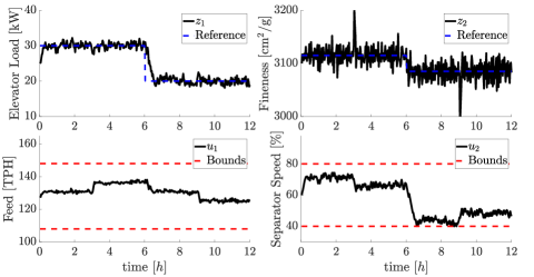
We implement the CT-MPC along with a linear Kalman filter on the simulated cement mill system. The covariance matrix of the measurement noise is $R_{vv}=\left[0.1;50\right]$ and the process noise covariance $R_{ww}$ is obtained from the differential equation $R_{ww}(T_{s})$. The cross-covariance matrix is assumed to be $S=0$. Fig. 1 illustrates the closed-loop simulation result of the cement mill system. Initially, the CT-MPC takes a while to bring two outputs to the reference (indicated by the blue lines). Then, there are overshoots on the outputs at $t=3$ [h] caused by the disturbance $d_{k}$. The controller captures the unknown disturbance and rejects it after a few iterations. The references have a step change at $t=6$ [h], and the system outputs are controlled to follow the new reference points. We withdraw the disturbance at $t=9$ [h]. Thus, the overshoots appear again, and the controller successfully handles it.

5 Conclusions

This paper introduced the discretization of continuous-time LQ-OCPs with time delays. We expressed the discrete weight matrices as the systems of differential equations, leading to the discrete equivalent of the continuous-time LQ-OCPs with time delays. Three numerical methods are described for solving proposed differential equation systems. We tested the CT-MPC with proposed numerical methods in the numerical experiment on a simulated cement mill system. The step-doubling is the fastest among all three methods and keeps the same accuracy level as the fixed-time-step ODE method. The closed-loop simulation results indicate that the proposed CT-MPCs can stabilize and control the simulated cement mill system.

References

  • Al-Mohy and Higham (2010) Al-Mohy, A.H. and Higham, N.J. (2010). A new scaling and squaring algorithm for the matrix exponential. SIAM Journal on Matrix Analysis and Applications, 31(3), 970–989.
  • Al-Mohy and Higham (2011) Al-Mohy, A.H. and Higham, N.J. (2011). Computing the action of the matrix exponential, with an application to exponential integrators. SIAM Journal on Scientific Computing, 33(2), 488–511.
  • Åström (1970) Åström, K.J. (1970). Introduction to stochastic control theory. Academic Press New York.
  • Åström and Wittenmark (2011) Åström, K.J. and Wittenmark, B. (2011). Computer-Controlled Systems: Theory and Design, Third Edition. Dover Publications.
  • Capolei et al. (2015) Capolei, A., Foss, B., and Jørgensen, J.B. (2015). Profit and risk measures in oil production optimization. IFAC-PapersOnLine, 48(6), 214–220. 2nd IFAC Workshop on Automatic Control in Offshore Oil and Gas Production OOGP 2015.
  • Franklin et al. (1990) Franklin, G.F., Powell, J.D., and Workman, M.L. (1990). Digital Control of Dynamic Systems. Electrical and Computer Engineering; Control Engineering. Addison-Wesley, Reading Massachusetts.
  • Frison and Jørgensen (2013) Frison, G. and Jørgensen, J.B. (2013). Efficient implementation of the riccati recursion for solving linear-quadratic control problems. In 2013 IEEE International Conference on Control Applications (CCA), 1117–1122.
  • Gu et al. (2003) Gu, K., Kharitonov, V.L., and Chen, J. (2003). Stability of Time-Delay Systems. Birkhäuser.
  • Hendricks et al. (2008) Hendricks, E., Sørensen, P.H., and Jannerup, O. (2008). Linear Systems Control: Deterministic and Stochastic Methods. Springer, Berlin, German.
  • Higham (2005) Higham, N.J. (2005). The scaling and squaring method for the matrix exponential revisited. SIAM Journal on Matrix Analysis and Applications, 26(4), 1179–1193.
  • Jørgensen et al. (2012) Jørgensen, J.B., Frison, G., Gade-Nielsen, N.F., and Damman, B. (2012). Numerical methods for solution of the extended linear quadratic control problem. IFAC Proceedings Volumes, 45(17), 187–193. 4th IFAC Conference on Nonlinear Model Predictive Control.
  • Jørgensen and Jørgensen (2007a) Jørgensen, J.B. and Jørgensen, S.B. (2007a). Comparison of Prediction-Error-Modelling Criteria. In American Control Conference 2007, 140–146.
  • Jørgensen and Jørgensen (2007b) Jørgensen, J.B. and Jørgensen, S.B. (2007b). Continuous-Discrete Time Prediction-Error Identification Relevant for Linear Model Predictive Control. In European Control Conference 2007, 4752–4758.
  • Jørgensen and Jørgensen (2007c) Jørgensen, J.B. and Jørgensen, S.B. (2007c). MPC-Relevant Prediction-Error Identification. In American Control Conference 2007, 128–133.
  • Kassas and Dunia (2006) Kassas, Z.M. and Dunia, R. (2006). Discretization of mimo systems with nonuniform input and output fractional time delays. In Proceedings of the 45th IEEE Conference on Decision and Control, 2541–2546. IEEE.
  • Lee (1995) Lee, E. (1995). Time-delay systems: Stability and performance criteria with applications: By j. e. marshall, h. górecki, k. walton and a. korytowski. ellis horwood, chichester (1992). Automatica, 31(5), 793–795.
  • Moler and Van Loan (1978) Moler, C. and Van Loan, C. (1978). Nineteen dubious ways to compute the exponential of a matrix. SIAM Rev., 20(4), 801–836.
  • Moler and Van Loan (2003) Moler, C. and Van Loan, C. (2003). Nineteen dubious ways to compute the exponential of a matrix, twenty-five years later. SIAM Review, 45(1), 3–49.
  • Olesen et al. (2013) Olesen, D.H., Huusom, J.K., and Jørgensen, J.B. (2013). A tuning procedure for arx-based mpc of multivariate processes. In 2013 American Control Conference, 1721–1726.
  • Otto and Radons (2017) Otto, A. and Radons, G. (2017). Time Delay Systems: Theory, Numerics, Applications, and Experiments. Springer.
  • Pannocchia et al. (2015) Pannocchia, G., Rawlings, J.B., Mayne, D.Q., and Mancuso, G.M. (2015). Whither discrete time model predictive control? IEEE Transactions on Automatic Control, 60(1), 246–252.
  • Pannocchia et al. (2010) Pannocchia, G., Rawlings, J.B., Mayne, D.Q., and Marquardt, W. (2010). On computing solutions to the continuous time constrained linear quadratic regulator. IEEE Transactions on Automatic Control, 55(9), 2192–2198.
  • Prasath et al. (2010) Prasath, G., Recke, B., Chidambaram, M., and Jørgensen, J.B. (2010). Application of soft constrained mpc to a cement mill circuit. IFAC Proceedings Volumes, 43(5), 302–307. 9th IFAC Symposium on Dynamics and Control of Process Systems.
  • Rockafellar and Uryasev (2001) Rockafellar, R. and Uryasev, S. (2001). Conditional value-at-risk: Optimization approach. Stochastic optimization: algorithms and applications, 411–435.
  • Van Loan (1978) Van Loan, C. (1978). Computing integrals involving the matrix exponential. IEEE Transactions on Automatic Control, 23(3), 395–404.