Role of Noise in the Fairen-Velarde model of bacterial respiration
Soumyadeep Kundu1 and Muktish Acharyya2,∗
Department of Physics, Presidency University,
86/1 College Street, Kolkata-700073, India Email1:sdpknu@gmail.com
Email2:muktish.physics@presiuniv.ac.in
Abstract: Following our recent study (Kundu and Acharyya, Int. J. Mod. Phys. C (2024) 2450094), we have introduced stochasticity (random noise) in the Fairen-Velarde deterministic differential equations. The role of such noise on time scales is studied. The probability of reaching the domain of fixed points in a given interval is also calculated. The probability is studied as a function of the width of the noise, and a hyperbolic tangent fitting is proposed. The noise reduces the time scale for bringing the bacteria into an inactive state. The area of the fixed-point domain was found to be asympotically linear with noise. The time to reach the fixed-point domain is fitted to a Gaussian with noise intensity.
Keywords: Klebsiella, Bacterial respiration, Fairen-Velarde model, Runge-Kutta- Fehlberg method, Fixed point, Limit cycle, Time scale, Noise
∗ Corresponding author
1 Introduction
The study of bacterial respiration is crucial for understanding various biological processes and ecological dynamics. Bacteria play vital roles in nutrient cycling, decomposition, and maintaining ecosystem stability. Besides, bacteria are also responsible for different diseases. One of the fundamental aspects of bacterial respiration involves the dynamics of oxygen and nutrient concentrations, which are essential for bacterial survival and growth.
In the realm of theoretical biology, mathematical models serve as valuable tools for understanding the complex dynamics of biological systems. The Fairen-Velarde model, proposed in 1979[1], is a notable example in the study of bacterial respiration. This model provides a mathematical framework to describe the interplay between oxygen and nutrient concentrations in bacterial populations.
The Fairen-Velarde model consists of a set of coupled nonlinear differential equations that capture the dynamics of oxygen and nutrient concentrations over time. These equations incorporate parameters such as transport rates, supply rates, and regulatory factors that influence the behaviour of the bacterial population.
In recent years, there has been growing interest in exploring the role of stochastic factors, such as noise, in biological systems. Noise can arise from various sources, including fluctuations in environmental conditions and inherent stochasticity in biochemical processes. Understanding how noise affects the dynamics of bacterial respiration can provide insights into the resilience and adaptability of bacterial populations in changing environments[2, 3, 4].
In this study, we investigate the role of noise in the Fairen-Velarde model of bacterial respiration. We explore how random fluctuations in oxygen and nutrient concentrations influence the stability and behaviour of the bacterial population. Through numerical simulations and statistical analysis, we analyze the effects of noise width and time scale on the dynamics of the system.
Our findings contribute to a broader understanding of bacterial respiration dynamics and provide insights into the mechanisms underlying the robustness and variability of bacterial populations. By integrating mathematical modelling with experimental data, we can gain deeper insights into the complex dynamics of microbial communities and their ecological significance.
2 Fairen-Velarde Mathematical model of Bacterial respiration
Theoretically, finding an appropriate model is necessary in order to analyse the bacterial life cycles. The time dependency of nutrition and oxygen amounts—two essential components for bacterial survival—must be provided by this model. Such dynamical evolution could be modelled by differential equations involving these two variables (nutrient and oxygen concentrations). Furthermore, a differential equation model of this kind ought to reflect the interdependence of these two fundamental variables. The most well-known model for bacterial respiration in this context is the Fairen-Velarde (1979) model[1].
| (1) |
In this case, the concentration of oxygen in the system is , whereas the concentration of nutrients is . The oxygen transport rate from the chamber to the system is represented by , and the reverse transport rate is represented by . The rate at which nutrients are supplied from the chamber to the system is . The limit cycle is determined by and . The concentrations of nutrients and oxygen in the chamber are and , respectively.
We have found the non-dimensionalized equation in our previous paper[7]
| (2) |
2.1 Ranges of parameters
All the parameters are positive definite because (since every term is dependent upon rate constants). So our conditions become,
| (3) | ||||
| (4) |
To have a stable fixed point, the aforementioned relationships must be upheld. The limit cycle can be found by extending outside of the previously specified range. To verify stability (or limit cycle), we evaluated the parameters in various ranges. Using the parameters from (eqn.(4)), we simulated[7] the nonlinear equation (eqn.(2)) using the 6-th order Runge-Kutta-Fehlberg method.
Now we are introducing time-dependent random noise to the system. So the equations will be transformed to
| (5) |
Here, the white noise is added with a mean value of zero, or . , , , . In the next section of this work, we will talk about the results of noises ranging in width from to at various time steps. The distribution of the noise width is uniform around zero. In every instance, the noise width is also of the same order. For example, it distributes between and if the noise width is .
3 Numerical Results of Fairen-Velarde coupled nonlinear differential equations
We have solved eqn. (1) using the 6th order Runge-Kutta-Fehlberg technique to get the instantaneous value of population (both and ) as a function of time(). We have used the 6th order Runge-Kutta-Fehlberg technique[6], mentioned above. We have taken the time interval so that the error involved in the 6th order RKF method is quite small.
3.1 Numerical results without noise
We have solved the eqn. (5) by the 6-th-order Runge-Kutta-Fehlberg method for the fixed set of values of the parameters, and the results are shown in Fig. 1. In these values of the parameters (, , and ), we have shown the existence of the stable limit cycle for a noiseless system. First of all, we shall take a noiseless system ().
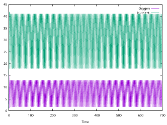
(a)
 (b)
(b)
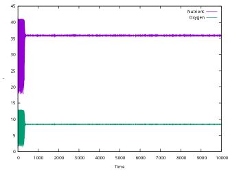
3.2 Reduction of Time-Scale in the presence of noise
By fixing our parameters, , , and , we are creating a limit cycle that will bring this system to a fixed point with even the smallest variation on one side. The system may be shifted to either side because we are providing random noise while maintaining a zero mean value. Macroscopically, the system should remain in equilibrium and there won’t be any net value of noise. However, we are seeing that the system may eventually approach a fixed point for the same noise width if a particular level of noise is applied for an extended period of time. Therefore, we must handle it statistically using a sizable amount of datapoints. To obtain sufficient samples for lower noise widths, we have taken ensembles for each noise. The five time limitations that we are computing the probability for are , , , , and .

(a)
 (b)
(b)
4 Analysis of the results
We will talk about the outcomes of our statistical analysis in this part. Reaching a fixed point is not a guarantee, as was previously mentioned. Thus, we will calculate the likelihood that it will reach the fixed point. Furthermore, we are unable to refer to it as a “fixed point” because the system is stuck in a “fixed region”, which we will refer to as a “fixed domain” in the material that follows, rather than reaching a ”unique” point. We designate it as a fixed domain if the successive peak-deep value of the nutrient and oxygen is 0.02 times that of the maximum peak-deep value. We will also examine how the fixed domain’s area varies with noise width. Lastly, we will investigate the approximate time required to get to the fixed point for each noise width.
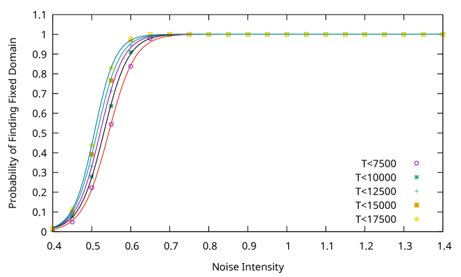
4.1 Probability to reach the fixed-point domain
We have measured the likelihood () of arriving at a given domain in various time frames. It appears that after a cutoff noise, it will undoubtedly go to the fixed domain. The following is the probability’s dataset: We are seeing a steady increase in at various noise levels based on our dataset. Our datapoints have now been fitted using the equation;
| (6) |
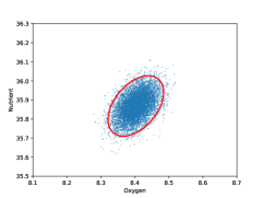
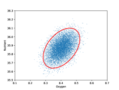
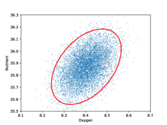
4.2 Area of the fixed domain
The system is not arriving to a single, fixed position, in contrast to the previous chapter. Rather, it is creating an ellipse area. We are now exploring the process of determining the region’s area. We shall take the Probabilistic Principal Component Analysis approach[8]. We will use an algorithm described in Fig. 4 to do this [9]. We will use our dataset to create a matrix. With N data points and k variables, the generalised matrix will be:
| (7) |
We are going to compute the covariance matrix now. One kind of matrix used to specify the covariance values between two items in random vectors is the covariance matrix. A definition of a covariance matrix () (a square matrix, indeed) is
| (8) |
where is the mean matrix (non-squared in general). This mean is calculated over various realisations of noise of fixed intensity. is defined as;
| (9) |
Now, we shall use the standard technique to determine the eigenvalues and eigenvectors of matrix. Now, if V is the eigenvector and is the eigenvalue,
| (10) |
From this, we can write,
| (11) |
So, we can identify the eigenvalues and subsequently find the eigenvectors from this process. Then we have to sort the eigenvalues and corresponding eigenvectors in descending order based on the magnitude of the eigenvalues.
Now, for our case, we have two variables i.e. Nutrient and Oxygen; denoting as N and O; the matrix will look like.
| (12) |
Now, the is a matrix, in general a non-square matrix. The covariant matrix will be a square square matrix. So, we shall get two eigenvalues of the covariant matrix , namely, and , with two eigenvectors and . So the rotation matrix can be given by eigenvectors as:
| (13) |
Again, can be also written in the terms of rotation angle() as,
| (14) |
Now, to get the semi-major axis of the ellipse, we shall consider the eigenvector corresponding to the larger eigenvalue, where as the smaller eigenvalue corresponds to the semi-minor axis. We can see that, the two rotation matrices mentioned in Eq. 13 and 14 are equivalent. So taking the first column, we can calculate,
| (15) |
So, from this we can calculate the angle of rotation of the ellipse.
Now we have to calculate the standard deviation of the principal components to find the dispersion of the set of values. Eigenvalues from the covariance matrix is the variation of the principle components; so if we take its square root, we shall get the standard deviation. So mathematically,
| (16) | |||
| (17) |
Now, we have to measure the scaling factor. For this, we are taking confidence limit i.e. we are taking data as outliers. Scaling factor() and confidence limit() is related as such,
| (18) |
Now, we have , and . So using this we can find the semi-major() and semi-minor() axes. The mathematical equation to find it is,
| (19) | |||
| (20) |
So, the area of the desired ellipse() can be calculated as,
| (21) |
(a)
 (b)
(b)
 (c)
(c)
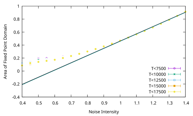
When we increase the noise, we see that the area gradually increases. For increased noise, we are seeing an asymptotic convergence of the data points to a straight line. Thus, we have used the equation 22 to fit the data points for noises larger than .
| (22) |
4.3 Time to reach the fixed domain
For each noise, we have determined the average time it takes to achieve the fixed domain within various time constraints. For averaging, we have only included ensembles that have reached the defined domain. We are observing there is a peak in between and . To observe it more specifically, we have fit it with the equation ,
| (23) |
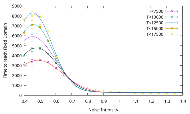
We observing that the system is obviously going to the fixed domain for higher noises asymptotically. There is a saturation of timescale at higher noises. It is taking time around 250-300 to reach the fixed domain.
5 Summary and concluding remarks
The Fairen-Velarde model is a prototypical model of bacterial respiration. The two-dimensional deterministic nonlinear differential equation for the oxygen and the nutrient contents can grasp the essential features of bacterial respirations. Depending on the various domains of the parameters, it can successfully provide the active phase (limit cycle) and the inactive phase (fixed point) of bacterial respiration. The existence of two time scales before reaching the fixed point has been shown in our previous work published in Int. J. Mod. Phys C (2024) 2450097.
In this article, we mainly focused on the role of noise in the steady behaviour of bacterial respiration. The stochasticity (introduced by noise) in the modified Fairen-Velrade model gives rise to various interesting phenomena. We have observed that the noise accelerates the motion towards the fixed point. We have shown the reduction of the gross time scale due to the presence of noise. This has far-reaching consequences in bacteriology. Just by introducing the noise (which may be thermal, impurity, or mechanical noise), one can bring the system of bacteria into an inactive phase (fixed point) faster than in a noiseless case.
The fixed point remains no longer a fixed point in the presence of noise. The scattering of fixed-point data covers a fixed-point domain in the presence of noise. The area of such a domain has been found to increase as the noise intensity is increased. Asymptotically, this growth is linear with noise intensity. To reach the fixed point, it becomes probabilistic with a given time in the presence of noise. The probality of reaching the fixed point domain within a given interval of time shows a hyperbolic tangent behaviour with noise intensity.
Acknowledgements:
Soumyadeep Kundu thankfully acknowledges the library facility of Presidency University, Kolkata.
Authors’ contribution:
Soumyadeep Kundu has developed the code for numerical calculations, collected data, prepared figures and written the manuscript. Muktish Acharyya has conceptualized the problem, analysed the results and written the manuscript.
Data availability statement: The data will be available on reasonable request to Soumyadeep Kundu.
Conflict of interest statement: We declare that this manuscript is free from any conflict of interest. The authors have no financial or proprietary interests in any material discussed in this article.
Funding statement: No funding was received particularly to support this work.
References
- [1] V. Fairen and M. G. Velarde, Time-periodic oscillations in a model for the respiratory process of a bacterial culture, J. Math. Biol. 8:2, 147-157, 1979.
- [2] Corinaldesi, C. (2015). New perspectives in benthic deep-sea microbial ecology. Frontiers in Marine Science, 2.
- [3] Ruwini Rupasinghe, Sathya Amarasena, Sudeera Wickramarathna, Patrick J. Biggs, Rohana Chandrajith, & Saumya Wickramasinghe (2022). Microbial diversity and ecology of geothermal springs in the high-grade metamorphic terrain of Sri Lanka. Environmental Advances, 7, 100166.
- [4] Horneck G, Klaus DM, Mancinelli RL. Space microbiology. Microbiol Mol Biol Rev. 2010 Mar;74(1):121-56. doi: 10.1128/MMBR.00016-09. PMID: 20197502; PMCID: PMC2832349.
- [5] Nonlinear dynamics and Chaos, S. H. Strogatz, (1994), Perseus Book publishing Limited, ISBN-0-201-54344-3
- [6] Applied Numerical analysis 7th edition, Curtis F. Gerald, Patrick O. Wheatley (2004), Pearson, ISBN-9780321133045
- [7] S. Kundu and M. Acharyya, Existence of two distinct time scales in the Fairen-Velarde model of bacterial respiration, Int. J. Mod. Phys. C, (2024), https://doi.org/10.1142/S0129183124500943
- [8] Tipping, M. E., & Bishop, C. M. (1999). Probabilistic Principal Component Analysis. Journal of the Royal Statistical Society. Series B (Statistical Methodology), 61(3), 611–622. http://www.jstor.org/stable/2680726
- [9] Bishop, Christopher M. (2006). Pattern recognition and machine learning. New York :Springer,