Enhanced Quantum Metrology with Non-Phase-Covariant Noise

Abstract

The detrimental impact of noise on sensing performance in quantum metrology has been widely recognized by researchers in the field. However, there are no explicit fundamental laws of physics stating that noise invariably weakens quantum metrology. We reveal that phase-covariant (PC) noise either degrades or remains neutral to sensing precision, whereas non-phase-covariant (NPC) noise can potentially enhance parameter estimation, surpassing even the ultimate precision limit achievable in the absence of noise. This implies that a non-Hermitian quantum sensor may outperform its Hermitian counterpart in terms of sensing performance. To illustrate and validate our theory, we present several paradigmatic examples of magnetic field metrology.

Introduction.—Investigating quantum parameter estimation in open systems is essential due to the unavoidable interaction of real physical systems with their surrounding environment [1, 2]. Previous studies consistently show that environmental noise degrades quantum coherence, leading to reduced sensing precision. Strategies such as dynamic decoupling [3, 4, 5, 6], time optimization [7, 8], quantum error correction [9, 10, 11], feedback control [12, 13, 14], quantum trajectory monitoring [15] and Floquet engineering [16] have been developed to overcome this challenge. Some works explore noise types with lesser detrimental effects, revealing that non-Markovian noises [17, 18, 19] or noises with special orientation [20] can be advantageous.

In fact, there is no fundamental law that prohibits the positive influence of environmental noise on quantum metrology. Recent findings recognize noise as a booster for quantum precision measurement and sensing in some cases [21, 22, 23, 24]. For instance, a high-temperature reservoir can enhance system fluctuations, improving distinguishability in measuring dual electron spin states [25]. The theory of enhanced sensor sensitivity at environmentally induced exceptional points has been experimentally validated [26, 27, 28], emphasizing the use of environmental factors to amplify quantum sensor responses to weak signals. Moreover, a dissipative adiabatic measurement based on noise is proposed [29], where noise is an indispensable resource.

Spirited by the development of noisy quantum metrology, two important questions naturally arise: (1) What types of noise may boost quantum metrology; (2) Can estimation precision in the presence of noise surpass the noiseless precision limit? This Letter aims to address these two questions. Firstly, we demonstrate that only NPC noise is likely to boost quantum metrology, while PC noise has a negative effect (or no effect) on sensing performance. Surprisingly, we find that the sensing precision of a non-Hermitian sensor influenced by NPC noise may surpass the ultimate precision limit given by its Hermitian counterpart. We illustrate these findings in the analysis of paradigmatic quantum metrological schemes, including quantum estimation of magnetic field strength and its direction. We emphasize that, unless otherwise stated, the noise mentioned below does not contain estimated parameters.

Preliminaries.—The dynamic evolution of an open quantum system is described by the master equation [30] $\partial_{t}\hat{\rho}\left(t\right)=(\hat{\mathcal{H}}+\hat{\mathcal{L}})\left[\hat{\rho}\left(t\right)\right]$ (hereafter $\hbar=1$), where $\hat{\mathcal{H}}\left[\bullet\right]:=-i[\hat{H},\bullet]$ and $\hat{\mathcal{L}}\left[\bullet\right]:=\sum_{k}\gamma_{k}[\hat{\Gamma}_{k}\bullet\hat{\Gamma}_{k}^{\dagger}-\frac{1}{2}\{\hat{\Gamma}_{k}^{\dagger}\hat{\Gamma}_{k},\bullet\}]$, with $\hat{H}$ the Hamiltonian of system and $\hat{\Gamma}_{k}$ the quantum jump operator associated with a dissipative channel occurring at decay rate $\gamma_{k}$. The series solution of $\hat{\rho}\left(t\right)$ reads as [31]

$$\hat{\rho}\left(t\right)=e^{\mathcal{\hat{H}}t}[\hat{\Pi}\left(t\right)[\hat{\rho}\left(0\right)]],$$ (1)

where $\hat{\rho}\left(0\right)$ is the initial-state density matrix operator of system, $\hat{\Pi}\left(t\right)=\sum_{n=1}^{\infty}(\hat{\mathbb{1}}+\hat{\Xi}_{n})$ is an effective dissipative superoperator, $\hat{\mathbb{1}}$ is identity superoperator, and

$$\hat{\Xi}_{n}=\int_{0}^{t}\int_{0}^{t_{1}}\cdots\int_{0}^{t_{n-1}}e^{-\mathcal{\hat{H}}t_{1}}\hat{\mathcal{L}}e^{\mathcal{\hat{H}}t_{1}}e^{-\mathcal{\hat{H}}t_{2}}\hat{\mathcal{L}}e^{\mathcal{\hat{H}}t_{2}}\cdots e^{-\mathcal{\hat{H}}t_{n}}\hat{\mathcal{L}}e^{\mathcal{\hat{H}}t_{n}}d{t_{n}}d{t_{n-1}}\cdots d{t_{1}}(n>0),$$ (2)

with the integral upper limit satisfying $t>t_{1}>\cdots>t_{n-1}$. Based on the commutativity of noise-induced operations with Hamiltonian dynamics in the master equation, noise is categorized into two types. The first one is PC noise, where dissipative dynamics commutes with coherent dynamics [32], i.e, $\mathcal{\hat{H}}[\mathcal{\hat{L}}[\hat{\rho}(t)]]=\mathcal{\hat{L}}[\mathcal{\hat{H}}[\hat{\rho}\left(t\right)]]$. In this case $\hat{\rho}\left(t\right)$ can be expressed as [31],

$$\hat{\rho}\left(t\right)=e^{\mathcal{\hat{L}}t}[e^{\mathcal{\hat{H}}t}[\hat{\rho}\left(0\right)]]=e^{\mathcal{\hat{L}}t}[\hat{\rho}^{\left(0\right)}\left(t\right)],$$ (3)

where $\hat{\rho}^{\left(0\right)}\left(t\right)$ represents the evolved state in the noiseless case. This implies a complete separation of the two dynamics in time evolution, and their order does not affect the final state $\hat{\rho}\left(t\right)$.

The other is NPC noise, where the two dynamics are no longer commutative [32], i.e., $\mathcal{\hat{H}}[\mathcal{\hat{L}}[\hat{\rho}(t)]]\neq\mathcal{\hat{L}}[\mathcal{\hat{H}}[\hat{\rho}(t)]]$. In this case, the two dynamics cannot be separated in state evolution, presenting significant challenges for solving the master equation. But at the short-term limit, $\hat{\rho}\left(t\right)$ is approximated as [31]

$$\hat{\rho}\left(t\right)\approx e^{\mathcal{\hat{H}}t}[e^{\mathcal{\hat{L}}t}[\hat{\rho}\left(0\right)]].$$ (4)

The approximate expression involves transforming the two concurrent dynamics processes into a sequential order, with dissipative dynamics preceding the coherent dynamics. This sequence implies that the noise may solely alter the effective initial state which subsequently undergoes coherent evolution.

Let $\theta$ represents the estimated parameter, and the corresponding estimation error is quantified by quantum Cramér-Rao bound (QCRB) [33], i.e., Var$(\hat{\theta})\geq 1/\nu F_{\theta}$. Here, Var$(\hat{\theta})$ is the mean squared error of unbiased estimator, $\nu$ is the number of trials, $F_{\theta}[\hat{\rho}_{\theta}]:=\text{Tr}[\hat{\rho}_{\theta}\hat{L}_{\theta}^{2}]$ is quantum Fisher information (QFI), and $\hat{L}_{\theta}$ is the symmetric logarithmic derivative formally defined by $\partial_{\theta}\hat{\rho}_{\theta}=(\hat{\rho}_{\theta}\hat{L}_{\theta}+\hat{L}_{\theta}\hat{\rho}_{\theta})/2$. The QCRB indicates the larger the QFI, the higher the theoretically achievable estimation precision of the sensor.

Non-phase-covariant noise enhanced sensing performance.—Assuming $\theta$ is only included in the Hamiltonian, superoperator $\hat{\mathcal{H}}\rightarrow\hat{\mathcal{H}}(\theta)$. Liouvillian superoperator $\mathcal{\hat{L}}$ is negative semidefinite when $\gamma_{k}\ \geq 0$ for $\forall k$ [30]. Its eigenvalues $\zeta_{k}$ and eigenmatrices $\hat{\Re}_{k}$ satisfy eigenequation $\mathcal{\hat{L}}\hat{\Re}_{k}=\zeta_{k}\hat{\Re}_{k}$ where $\mathbb{R}$e$\left[\zeta_{k}\right]\leq 0$ for $\forall k$, leading to $0\leq e^{\mathbb{R}\text{e}\left[\zeta_{k}\right]}\leq 1$ and a potential decrease in the elements of the density matrix. Thus, for PC noise, based on Eq. (3) and the definition of the QFI we can conclude that

$$F_{\theta}\left[\hat{\rho}_{\theta}\left(t\right)\right]\leq F_{\theta}[\hat{\rho}_{\theta}^{\left(0\right)}\left(t\right)].$$ (5)

The formula indicates that PC noise is detrimental to estimation precision, or at best, it does not affect it. This is because if information about $\theta$ in $\hat{\rho}_{\theta}^{\left(0\right)}\left(t\right)$ is not encoded in a decoherence-free subspace, it leaks to the environment, resulting in a decrease in estimation precision.

For NPC noise, a positive answer to question 1 can be obtained by studying the following limiting scenario through Eq. (4). Suppose initial state $\hat{\rho}\left(0\right)$ is an eigenstate of Hamiltonian $\hat{H}\left(\theta\right)$, without $e^{\mathcal{\hat{L}}t}$ we can’t extract any information about $\theta$ from state $\hat{\rho}(t)$ since it only manifests as a global phase factor. However, introducing NPC noise causes $\hat{\rho}(0)$ to deviate from the eigenstate, and $\theta$ is subsequently encoded into $\hat{\rho}(t)$ under the action of $e^{\mathcal{\hat{H}}\left(\theta\right)t}$. This results in $F_{\theta}\left[\hat{\rho}_{\theta}\left(t\right)\right]\neq 0$, signifying that NPC noise enables previously unattainable quantum parameter estimation. Furthermore, if $\hat{\rho}\left(0\right)$ is not the optimal initial state, the action of $e^{\mathcal{\hat{L}}t}$ may bring $\hat{\rho}\left(0\right)$ closer to the optimal state, leading to enhanced estimation precision.

Now, addressing question 2: Can the sensing precision of a non-Hermitian sensor with NPC noise surpass its Hermitian counterpart’s limit? If the noise itself includes the estimated parameter, a positive answer is not surprising, as recent research has also confirmed [34]. This Letter focuses on the case where the noise lacks the estimated parameter. Unfortunately, this situation cannot be analyzed solely from Eq. (4). This is because, under the encoding by the Hamiltonian, the performance of the effective initial state $e^{\mathcal{\hat{L}}t}[\hat{\rho}\left(0\right)]$ cannot surpass that of the optimal initial state in a closed system. To address this, we must delve into the high-order corrections introduced by NPC noise. Perform the following substitution in Eq. (1): $\hat{\mathcal{H}}\rightarrow\hat{\mathcal{H}}(\theta)$ and $\hat{\Pi}\left(t\right)\rightarrow\hat{\Pi}\left(\theta,t\right)$. In this case, $\hat{\Pi}\left(\theta,t\right)$ is an effective dissipative superoperator containing the estimated parameter, implying an additional parameter encoding process beyond coherent dynamics. Then a conclusion can be drawn that the estimation precision obtained from an open quantum system with NPC noise may surpass the precision limit determined by the optimal initial state and optimal estimation time of its closed counterpart, expressed as

$$F_{\theta}\left[\hat{\rho}_{\theta}\left(\tau\right)\right]>F_{\theta}\left[e^{\mathcal{\hat{H}}\left(\theta\right)t_{\text{optl}}}\hat{\rho}^{\text{optl}}\left(0\right)\right],$$ (6)

may hold. Here, $\tau$ is a moment that depends on the specific form of the Hamiltonian and NPC noise. $\hat{\rho}^{\text{optl}}\left(0\right)$ and $t_{\text{optl}}$ represent the optimal initial state and the optimal encoding time in the closed system, respectively. This surprising result contradicts intuition, as noise without estimated parameters can assist sensors in surpassing the precision limit established by coherent dynamics. Physically, this stems from NPC noise introducing an additional parameter encoding process, capitalizing on the non-commutativity between coherent and dissipative dynamics, compared to the noiseless case.

Example—Consider an open spin-$1/2$ system, whose dynamics is governed by a generalized master equation,

$$\frac{d\hat{\rho}\left(t\right)}{dt}=-i[\hat{H}_{\text{S}},\hat{\rho}\left(t\right)]+\gamma[\hat{\Gamma}\hat{\rho}\left(t\right)\hat{\Gamma}^{{\dagger}}-\frac{1}{2}\{\hat{\Gamma}^{{\dagger}}\hat{\Gamma},\hat{\rho}\left(t\right)\}],$$ (7)

where $\hat{H}_{\text{S}}=B\left[\cos(\vartheta)\hat{\sigma}_{x}+\sin(\vartheta)\hat{\sigma}_{z}\right]$ is the Hamiltonian of the system, with the Bohr magneton set to $1$ for simplicity. $B$ and $\vartheta$ denote the amplitude and direction of the magnetic field in the $XZ$ plane, respectively. $\hat{\Gamma}=\cos(\alpha)\hat{\sigma}_{x}+\sin(\alpha)\hat{\sigma}_{z}$ is general quantum jump operator [35, 36], where $\alpha$ is the coupling angle between the spin and environment bath. $\hat{\sigma}_{x,z}$ and $\gamma$ are the Pauli operator and the decay rate, respectively. The model can be experimentally implemented using atoms or quantum dots [37, 38], where atoms or electron spins are simultaneously excited and relaxed, accompanied by phase diffusion due to random fluctuations in the electromagnetic environment.

Scenario 1: when $\vartheta=\alpha=\pi/2$, the Hamiltonian $\hat{H}_{\text{S}}=B\hat{\sigma}_{z}$, the jump operator $\hat{\Gamma}=\hat{\sigma}_{z}$, and $[\hat{H}_{\text{S}},\hat{\Gamma}]=0$ i.e., the system is affected by PC noise. Suppose initial state of system is $\left|\Phi\left(0\right)\right\rangle=\cos(\frac{\beta}{2})\left|e\right\rangle+\sin(\frac{\beta}{2})\left|g\right\rangle$, where $\hat{\sigma}_{z}\left|e\right\rangle=\left|e\right\rangle$ and $\hat{\sigma}_{z}\left|g\right\rangle=-\left|g\right\rangle$. Let $\beta$ and $B$ be the estimated parameters, the QFI for each parameter reads

$$F_{\beta}\left[\hat{\rho}\left(t\right)\right] = 1,$$ (8a)

$$F_{B}\left[\hat{\rho}\left(t\right)\right] = 4\sin^{2}(\beta)e^{-4\gamma t}t^{2},$$ (8b)

One can see that the PC noise has no effect on the estimation precision of $\beta$ but reduces that of $B$. These results are consistent with the conclusions presented earlier.

Scenario 2: when $\vartheta=\pi/2$ and $\alpha\neq k\pi/2$ $(k\in\mathbb{Z})$, $\hat{\Gamma}$ in this case signifies NPC noise. Suppose initial state is $\left|\Phi\left(0\right)\right\rangle=\left|g\right\rangle$, the corresponding Bloch vector is $\vec{r}\left(0\right)=\left[0,0,-1\right]^{\text{T}}$, lying on the negative $Z$ axis. In the noiseless case, one can’t get information of $B$ from evolved states because $\left|\Phi\left(t\right)\right\rangle=e^{iBt}\left|g\right\rangle$ and $F_{B}\left[\hat{\rho}(t)\right]=0$. The non-commutative nature of NPC noise presents challenges in obtaining analytical expressions for $\hat{\rho}(t)$ and subsequently QFI. However, at the short-term limit, the Bloch vector of the system can be approximately solved [39], i.e,

$$\vec{r}\left(t\right)=\Upsilon_{\text{npc}}\left(t\right)\vec{r}\left(0\right)=-\left[\Upsilon_{13},\Upsilon_{23},\Upsilon_{33}\right]^{\text{T}},$$ (9)

where $\Upsilon_{\text{npc}}$ represents the affine transformation matrix of the Bloch sphere, it signifies unequal contractions along the $X$, $Y$, and $Z$ axes, along with rotations around certain axes. Consequently, $\vec{r}(t)$ diverges from the $Z$ axis, acquiring quantum coherence and encoding effective information about $B$. The matrix elements $\Upsilon_{13}$ and $\Upsilon_{23}$ contain parameter $B$, leading to $F_{B}\left[\hat{\rho}\left(t\right)\right]\neq 0$. This indicates that the NPC noise can boost quantum metrology. Furthermore, the presence of non-zero $\Upsilon_{13}$ and $\Upsilon_{23}$ indicates that the NPC noise imparts quantum coherence. This arises from the fact that the correlation between the decay channels through $\hat{\sigma}_{x}$ and $\hat{\sigma}_{z}$ in $\hat{\Gamma}$ is established by the dissipation process $\hat{\Gamma}\hat{\rho}(t)\hat{\Gamma}^{\dagger}$. For PC noise, the affine transformation matrix $\Upsilon_{\text{pc}}$ shrinks the Bloch sphere equally along the $X$ and $Y$ axes and rotates around the $Z$ axis, making the Bloch vector $\vec{r}\left(t\right)$ always follow the $Z$ axis without containing effective information about $B$. See Supplemental Material for specific forms of $\Upsilon_{\text{pc}}$ and $\Upsilon_{\text{npc}}$ [39]. Notice that, not all NPC noises can lead to the above results, e.g., $\hat{\Gamma}=\hat{\sigma}_{x}$.

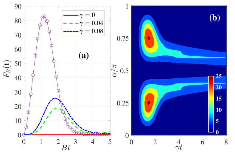
Figure 1: (a) $F_{B}$ versus encoding time $t$ with various decay rates, where $\alpha=\pi/4$ and $B=0.1$ (used as a scale). The purple circle line corresponds to the initial state $\left|\Phi\left(0\right)\right\rangle=(\left|g\right\rangle+\left|e\right\rangle)/\sqrt{2}$ , while the others correspond to $\left|\Phi\left(0\right)\right\rangle=\left|g\right\rangle$. (b) The density plot of $F_{B}$ versus $\alpha$ and $\gamma t$.

We present the variation of $F_{B}$ based on the exact numerical solution of the master equation in Fig. 1. Figure 1(a) illustrates that NPC noise significantly enhances $F_{B}$, indicating enhanced estimation precision when the initial state is $\left|\Phi\left(0\right)\right\rangle=\left|g\right\rangle$, and higher decay rates result in increased maximum value of $F_{B}$. But due to dissipation, $F_{B}$ eventually becomes zero over time. Interestingly, we observe that as the decay rate $\gamma$ increases, the value of $F_{B}$ derived from the initial state $\left|\Phi\left(0\right)\right\rangle=\left|g\right\rangle$ temporarily surpasses the value achieved with the noise-free optimal state $\left|\Phi\left(0\right)\right\rangle=(\left|g\right\rangle+\left|e\right\rangle)/\sqrt{2}$ over a specific duration. This suggests a potential metrological advantage of non-optimal states in practical noisy environments. From Fig. 1(b), we can see that the optimal coupling angle $\alpha_{\text{optl}}$ for the NPC noise-enhanced sensing precision is $\pi/4$ or $3\pi/4$. This is because when $\alpha=k\pi/4$ ($k$ is an odd number), the weights of $\hat{\sigma}_{x}$ and $\hat{\sigma}_{z}$ in the jump operator $\hat{\Gamma}$ are the same, maximizing the correlation between the two dissipation channels [39]. In addition, Fig. 1(b) exhibits symmetry with respect to $\alpha=\pi/2$, stemming from the fact that substituting $\alpha$ with $\pi-\alpha$ leaves the master Eq. (7) unaffected.

Scenario 3: Now, we consider the angle $\vartheta$ representing the direction of the magnetic field as the parameter to be estimated. We rewrite the Hamiltonian of system to $\hat{H}_{\text{S}}=\vec{R}\cdot\vec{J}$, where $\vec{R}=\left[2B\cos\left(\vartheta\right),0,2B\sin\left(\vartheta\right)\right]$ and $\vec{J}=\left[\hat{\sigma}_{x}/2,0,\hat{\sigma}_{z}/2\right]$. Utilizing the method developed by Wang et al. [40], the corresponding maximum QFI is given by

$$F_{\vartheta}^{\text{max}}\left(t\right)=\left(\frac{d|\vec{R}|}{d\vartheta}\vec{e}_{R}\right)^{2}t^{2}+4\left(\frac{d|\vec{e}_{R}|}{d\vartheta}\right)^{2}\text{sin}^{2}\left(\frac{|\vec{R}|}{2}t\right).$$ (10)

Since the magnitude of $\vec{R}$ is independent of $\vartheta$, the maximum noiseless QFI regarding $\vartheta$ expressed as $F_{\vartheta}=4\sin^{2}\left(Bt\right)$ which reaches the ultimate value of $4$ at the optimal encoding time $t_{\text{optl}}=\left(\pi/2+k\pi\right)/B$.

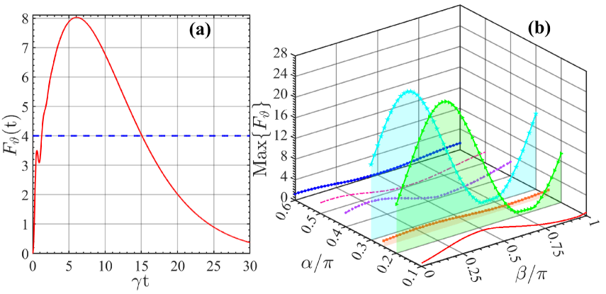
Figure 2: (a) $F_{\vartheta}$ (red solid line) versus encoding time $t$ in the presence of noise, where the magnetic field direction $\vartheta=\pi/3$, the noise coupling angle $\alpha=\pi/4$, $\beta=\pi/3$, $\gamma=0.03$ and $B=0.1$ (used as a scale). The blue dashed line denotes the noise-free maximum of $F_{\vartheta}$. (b) The maximum QFI as a function of $\alpha$ and $\beta$, where the magnetic field direction $\vartheta=\pi/4$ and other parameters are the same as (a). The orange curve corresponds to $\alpha=\vartheta$.

The primary effect of NPC noise on the QFI can also be demonstrated within this model by utilizing the reaction-coordinate polaron transform to introduce an effective Hamiltonian $\hat{H}_{\text{S}}^{\text{eff}}=\vec{R}^{\prime}\cdot\vec{J}$ [41]. This Hamiltonian accurately captures the dominant dynamics of the system within the open environment. We observe that unlike $\vec{R}$, both the magnitude and direction of $\vec{R}^{\prime}$ vary with $\vartheta$. Especially, the change in its magnitude leads to an accelerated increase in $F_{\vartheta}^{\text{max}}$ with a factor of $t^{2}$, far surpassing the $\sin^{2}(Bt)$ factor derived from directional changes, indicating a potential to exceed a maximum of noiseless QFI.

Fig. 2(a) shows the numerical simulation of $F_{\vartheta}$ evolving over time with noise, exceeding 4 for a specific duration. This verifies our theory that NPC noise can enhance the non-Hermitian sensor’s precision in measuring magnetic field direction beyond its Hermitian counterpart’s limit. Fig. 2(b) presents a 3D plot depicting the maximum ${F_{\vartheta}}$ as a function of both noise coupling angle $\alpha$ and initial state parameter $\beta$ in the noisy environment. These maximums represent the peaks throughout time evolution. The plot suggests that if there is a substantial difference between $\alpha$ and $\vartheta$, surpassing the precision limit is impossible, regardless of the chosen initial state. In contrast, when $\alpha$ is very close to $\vartheta$, it becomes more feasible to surpass the precision limit by selecting an appropriate initial state. However, this comes at the expense of requiring a longer encoding time. Fortunately, the open system takes a considerable time to decay to a steady state in this case, thereby affording an extended window for encoding [42]. But for the special case of $\alpha=\vartheta$, indicating the transition from NPC to PC noise, the highest precision limit set by coherent dynamics cannot be exceeded.

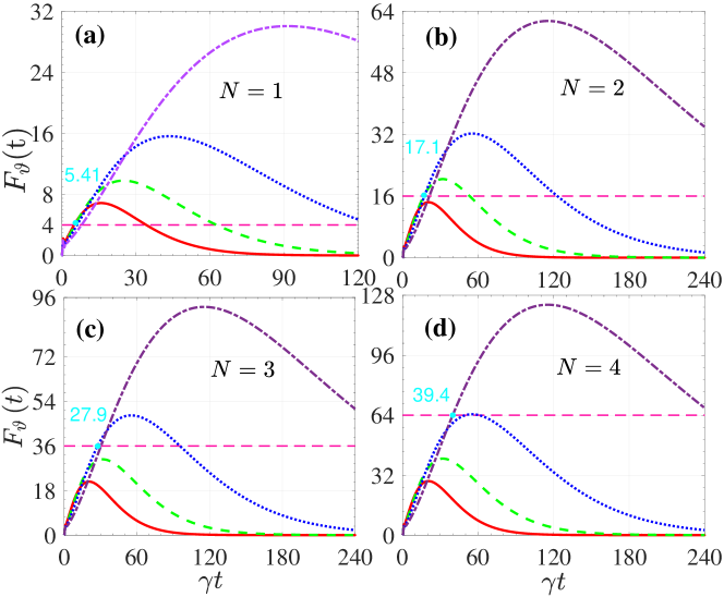
Figure 3: $F_{\vartheta}$ versus $\gamma t$ for different coupling angles $\alpha$, as the particle number $N$ increases, with magnetic field direction $\vartheta=\pi/3$. The red solid, green dashed, blue dotted, and purple dotted-dashed lines correspond to $\alpha=0.28\pi,0.29\pi,0.3\pi,0.31\pi$, respectively. The pink dashed lines in each subplot represent the maximum QFI set by the coherent dynamics, while the sky blue numbers indicate the time it takes to surpass them.

Multi-particle scenario—The results obtained in the previous section should also hold for collective systems composed of $N$ particles, as Eq. (1) is universal and does not confine the analysis to a specific model. To verify this, we simulated the corresponding $N$-particle master equation and computed the QFI [43], assuming no direct coupling between particles for generality. Fig. 3 plots the variation of $F_{\vartheta}$ with $\gamma t$ for different coupling angles $\alpha$, where the initial state of the system is $\left|\Phi_{\text{tot}}\left(0\right)\right\rangle=\left[\left(\left|e\right\rangle+\left|g\right\rangle\right)/\sqrt{2}\right]^{\otimes N}$ (For entangled initial states, see supplementary material for similar results.). We observe that for particle number $N=2,3,4$, as long as the coupling angle $\alpha$ is chosen appropriately, and with the aid of NPC noise, the estimation precision consistently exceeds the ultimate precision limit set by the optimal initial state (entangled state) in the absence of noise. However, it is worth noting that as $N$ increases, surpassing this limit through the introduction of NPC noise becomes progressively more challenging. This is because the selection of the coupling angle $\alpha$ becomes more stringent (manifested as $\alpha$ needing to be closer to $\vartheta$), and the encoding time also becomes longer (see the sky blue numbers), posing significant challenges for practical experimental realization. Notice that, in the absence of NPC noise, the maximum value of $F_{\vartheta}$ in an $N$-particle system is $4N^{2}$ (see the pink dashed lines). This implies that the precision limit can reach the Heisenberg scale in terms of particle number. Although NPC noise cannot break this scale, it can, in principle, make the $F_{\vartheta}$ value exceed $4N^{2}$.

Discussion and summary—More recently, a study reported that non-Hermitian sensors do not outperform their Hermitian counterparts in the performance of sensitivity [44]. The authors derived an upper bound of channel QFI, i.e., $F_{\lambda}^{\left(c\right)}\left(t\right)\leq\left[\int\nolimits_{0}^{t}||\partial\hat{H}_{\lambda}\left(s\right)/\partial\lambda||ds\right]^{2}=\mathcal{F}_{\lambda}^{\text{UB}}$, where $\hat{H}_{\lambda}\left(t\right)$ is the parameter-dependent Hamiltonian of the system, and $F_{\lambda}^{\left(c\right)}\left(t\right)$ is the maximum QFI achievable by optimizing the initial state. We point out that the equality sign in the above inequality can be achieved when the estimated parameter is the overall factor of the Hamiltonian [45], e.g., $\hat{H}_{B}=B\hat{\sigma}_{z}\Rightarrow F_{B}^{\left(c\right)}\left(t\right)=\mathcal{F}_{B}^{\text{UB}}=4t^{2}$. However, the estimated parameter is not always an overall multiplicative factor of the Hamiltonian, e.g., $\hat{H}_{\vartheta}=B\left[\cos(\vartheta)\hat{\sigma}_{x}+\sin(\vartheta)\hat{\sigma}_{z}\right]$. In this case, $F_{\vartheta}^{\left(c\right)}\left(t\right)=4\sin^{2}\left(Bt\right)$, well below the up bound $\mathcal{F}_{\vartheta}^{\text{UB}}=4B^{2}t^{2}$ for $t\gg 1$. Our study suggests that appropriate NPC noise can bridge this gap and enhance the precision limit, without violating the inequality.

In summary, we found that NPC noise can enhance quantum metrology due to the non-commutative nature between coherent and dissipative dynamics. Remarkably, the QFI attained through dynamics influenced by NPC noise can surpass the ultimate limit set solely by coherent dynamics. This suggests that the sensing precision of a non-Hermitian sensor with NPC noise can potentially outperform its Hermitian counterpart. Utilizing a general series solution analysis of the master equation, we establish the universality of our findings and demonstrate a specific instance of noise-enhanced magnetic-field quantum metrology. Furthermore, this approach provides valuable insights for enhancing other quantum technologies that are constrained by environmental noise.