Improved parameter selection strategy for the
iterated Arnoldi-Tikhonov method

Abstract

The iterated Arnoldi-Tikhonov (iAT) method is a regularization technique particularly suited for solving large-scale ill-posed linear inverse problems. Indeed, it reduces the computational complexity through the projection of the discretized problem into a lower-dimensional Krylov subspace, where the problem is then solved.

This paper studies iAT under an additional hypothesis on the discretized operator. It presents a theoretical analysis of the approximation errors, leading to an a posteriori rule for choosing the regularization parameter. Our proposed rule results in more accurate computed approximate solutions compared to the a posteriori rule recently proposed in [3]. The numerical results confirm the theoretical analysis, providing accurate computed solutions even when the new assumption is not satisfied.

1 Introduction

We study operator equations of the type

$$Tx=y,\quad x\in\mathcal{\mathcal{X}},\quad y\in\mathcal{Y},$$ (1)

where $T\colon\mathcal{\mathcal{X}}\to\mathcal{\mathcal{Y}}$ is a bounded linear operator between two separable Hilbert spaces which we assume to be not continuously invertible.

Let $T^{\dagger}$ be the Moore-Penrose pseudo-inverse of $T$, in particular

$$T^{\dagger}\colon\operatorname{dom}(T^{\dagger})\subseteq\mathcal{Y}\to\mathcal{X},\qquad\mbox{where }\operatorname{dom}(T^{\dagger})=\operatorname{Rg}(T)\oplus\operatorname{Rg}(T)^{\perp}.$$

For any $y\in\operatorname{dom}(T^{\dagger})$, the image $x^{\dagger}\coloneqq T^{\dagger}y$ is the unique least-square solution of the minimal norm of (1); it is referred to as the best-approximate solution. To ensure consistency in (1), we will assume as a base hypothesis that

$$y\in\operatorname{dom}(T^{\dagger}).$$

Since $T$ is not continuously invertible, the operator $T^{\dagger}$ is unbounded. Hence, the least-squares solution $x^{\dagger}$ is very sensitive to perturbations in $y$.

Moreover, the element $y$ in equation (1) is not available; we have information on an error-contaminated approximation $y^{\delta}\in\mathcal{Y}$ of $y$. We assume the inequality

$$\|y-y^{\delta}\|_{\mathcal{Y}}\leq\delta,$$

where $\|\cdot\|_{\mathcal{Y}}$ is the norm on $\mathcal{Y}$, with a known or estimated bound $\delta>0$. Therefore, our equation takes the form

$$Tx=y^{\delta},\quad\mbox{where }x\in\mathcal{X},\quad y^{\delta}\in\mathcal{Y}.$$ (2)

We would like to determine an accurate approximation of $x^{\dagger}$ by solving (2). To achieve this, equation (2) needs to be regularized, in order to obtain a well-posed problem. A regularization method replaces $T^{\dagger}$ by an operator in the collection $\{R_{\alpha}\colon\mathcal{Y}\to\mathcal{X}\}$ of continuous operators that depend on a parameter $\alpha$, associated to a parameter choice rule $\alpha=\alpha(\delta,y^{\delta})>0$. We can say that the pair $(R_{\alpha},\alpha)$ is a point-wise approximation of $T^{\dagger}$. Readers interested in an introduction to inverse problems regularization theory in Hilbert spaces can consult [7, 21].

Equations of the form (2) arise in many applications as remote sensing [1], atmospheric tomography [19], computerized tomography [14], adaptive optics [17], image restoration [2], etc.

Based on results by Natterer [13] and Neubauer [15], in [3] investigated the aforementioned problem addressing all discretization, approximation, and noise errors in the setting of iterated Tikhonov-like regularizations methods such as the iterated Arnoldi-Tikhonov method.

The operator equation (2) is firstly discretized, and the effect of the discretization is established based on the analysis by Natterer [13]. The resulting linear system of equations is assumed to be large and the matrix representing this system is subsequently reduced in size through the application of an Arnoldi decomposition. This reduced linear system is then regularized with the Tikhonov method. This strategy is largely explored in the literature of hybrid methods, e.g. [8, 12]. The error that arises from replacing the discretized system with a smaller one is studied in [18] using the results presented in [7].

It is well-known that iterative Tikhonov methods often produce computed approximate solutions of superior quality and show higher robustness when compared to standard Tikhonov regularization; see e.g. [5, 6, 10]. Therefore, in [3], the authors extend the results in [18] to the iterated Arnoldi-Tikhonov (iAT) method. The purpose of this paper is to give conditions on the operator in order to get faster convergence. We develop an analysis that checks all approximation errors. Our analysis leads to a different approach to determining the regularization parameter, improving the parameter choice method discussed in [3]. In detail, requiring a further assumption on the true solution, we prove that the reconstruction error obtained with our parameter estimation rule is lower with respect to the parameter estimated with the rule proposed in [3]. In other terms, it gives computed approximate solutions of higher quality. This is confirmed by the numerical results, where even when the new assumption is not satisfied, our proposal computes accurate reconstructions with Krylov subspaces of smaller dimensions compared to the proposal in [3], resulting in a lower computational cost.

This paper is organized as follows. Section 2 introduces a new a posteriori parameter estimation rule for the iterated Tikhonov method, based on a reasonable assumption about the true solution. Section 3 describes the approximation process, while Section 4 applies the previous analysis to the iAT method. The numerical tests in Section 5 compare the results obtained with the new parameter estimation rule with that proposed in [3]. Finally, Section 6 draws conclusions.

2 An a posteriori rule for the iterated Tikhonov method

We will denote with $\|\cdot\|_{\mathcal{X}}$ the norm on $\mathcal{X}$ and with $\|\cdot\|_{2}$ the Euclidean norm. The apex $\ast$ will denote the adjoint operator and $I$ will be the identity map where a subscript will indicate the dimension.

Assumption 2.1.

Let $T\in\mathcal{L}({\mathcal{X}},\mathcal{\mathcal{Y}})$ be a bounded linear operator. Consider a family $\{W_{m}\}_{m\in\mathbb{N}}$ of finite-dimensional subspaces of $\mathcal{X}$ such that the orthogonal projector $Q_{m}$ into $W_{m}$ converges to $I$ on $\mathcal{X}$.

Define the operator $T_{m}\coloneqq TQ_{m}$ and let $R_{m}$ be the orthogonal projector into $\operatorname{Rg}(T_{m})$ which converges to $I$ on $\operatorname{Rg}(T)$.

Using the iterated Tikhonov (iT) method (see [7, Section 5]) applied on equation (2) with $T_{m}$, we define the computed approximate solution

$$x_{\alpha,m,i}^{\delta}\coloneqq\sum\limits_{k=1}^{i}\alpha^{k-1}(T_{m}^{\ast}T_{m}+\alpha I)^{-k}T_{m}^{\ast}y^{\delta}$$ (3)

of (2).

For $\tau\geq 1$ consider the equation

$$\alpha^{2i+1}\langle(T_{m}T_{m}^{\ast}+\alpha I)^{-2i-1}R_{m}y^{\delta},R_{m}y^{\delta}\rangle=\tau\delta^{2}.$$ (4)

Similarly as in [3, Proposition A.6], one can show that there is a unique solution of (4) provided

$$\tau\delta^{2}<\|R_{m}y^{\delta}\|^{2}.$$ (5)

Proposition 2.2.

Let Assumption 2.1 and (5) be satisfied with $\tau=1$. If $R_{m}Tx^{\dagger}=T_{m}x^{\dagger}$ and $\alpha$ is the unique solution of (4), then for all $\tilde{\alpha}\geq\alpha$ holds $\|x^{\dagger}-x_{\alpha,m,i}^{\delta}\|\leq\|x^{\dagger}-x_{\tilde{\alpha},m,i}^{\delta}\|$.

Proof.

Let $\{F_{\mu}^{m}\}_{\mu\in\mathbb{R}}$ be a spectral family for $T_{m}T^{\ast}_{m}$ (see e.g. [7, Section 2.3]).

Define $e(\alpha)\coloneqq\frac{1}{2}\|x^{\dagger}-x_{\alpha,m,i}^{\delta}\|^{2}$, from the hypothesis follows $T_{m}x^{\dagger}=R_{m}Tx^{\dagger}=R_{m}y$, then

$$\frac{de(\alpha)}{d\alpha} =i\biggl{\langle}T_{m}x^{\dagger}-\int_{0}^{\infty}\frac{(\mu+\alpha)^{i}-\alpha^{i}}{(\mu+\alpha)^{i}}dF_{\mu}^{m}R_{m}y^{\delta},\int_{0}^{\infty}\frac{\alpha^{i-1}}{(\mu+\alpha)^{i+1}}dF_{\mu}^{m}R_{m}y^{\delta}\biggr{\rangle}$$

$$=i\biggl{\langle}R_{m}y-\int_{0}^{\infty}\frac{(\mu+\alpha)^{i}-\alpha^{i}}{(\mu+\alpha)^{i}}dF_{\mu}^{m}R_{m}y^{\delta},\int_{0}^{\infty}\frac{\alpha^{i-1}}{(\mu+\alpha)^{i+1}}dF_{\mu}^{m}R_{m}y^{\delta}\biggr{\rangle}.$$

Now, adding and subtracting $i\alpha^{2i-1}\|(T_{m}T_{m}^{\ast}+\alpha I)^{\frac{-2i-1}{2}}R_{m}y^{\delta}\|^{2}$ we obtain

$$\frac{de(\alpha)}{d\alpha}= i\alpha^{2i-1}\|(T_{m}T_{m}^{\ast}+\alpha I)^{\frac{-2i-1}{2}}R_{m}y^{\delta}\|^{2}$$

$$+i\biggl{\langle}\int_{0}^{\infty}\frac{\alpha^{i-1}}{(\mu+\alpha)^{\frac{1}{2}}}dF_{\mu}^{m}R_{m}(y-y^{\delta}),(T_{m}T_{m}^{\ast}+\alpha I)^{\frac{-2i-1}{2}}R_{m}y^{\delta}\biggr{\rangle}.$$

Thus, collecting $i\|(T_{m}T_{m}^{\ast}+\alpha I)^{\frac{-2i-1}{2}}R_{m}y^{\delta}\|\eqqcolon K$ from the two terms we have

$$\frac{de(\alpha)}{d\alpha}\geq K\left(\alpha^{2i-1}\|(T_{m}T_{m}^{\ast}+\alpha I)^{\frac{-2i-1}{2}}R_{m}y^{\delta}\|-\biggl{\|}\int_{0}^{\infty}\frac{\alpha^{i-1}}{(\mu+\alpha)^{\frac{1}{2}}}dF_{\mu}^{m}R_{m}(y-y^{\delta})\biggr{\|}\right)$$

and from

$$\biggl{\|}\int_{0}^{\infty}\frac{\alpha^{i-1}}{(\mu+\alpha)^{\frac{1}{2}}}dF_{\mu}^{m}R_{m}(y-y^{\delta})\biggr{\|}\leq\alpha^{i-\frac{3}{2}}\delta$$

the thesis follows. ∎

3 Discretization of the operator equation

In the case of real-world applications, the model equations (1) and (2) are discretized in order to compute an approximate solution. This process introduces a discretization error that we bound using results from Natterer [13]. We follow a similar approach as in [18], but applied to the iterative version of the Tikhonov method.

Consider a sequence $\mathcal{X}_{1}\subset\mathcal{X}_{2}\subset\ldots\subset\mathcal{X}_{n}\subset\ldots\subset\mathcal{X}$ of finite-dimensional subspaces, with dense union in $\mathcal{X}$ and $\dim(\mathcal{X}_{n})=n$. We define the projectors $P_{n}\colon\mathcal{\mathcal{X}}\to\mathcal{\mathcal{X}}_{n}$ and $Q_{n}\colon\mathcal{Y}\to\mathcal{Y}_{n}\coloneqq T(\mathcal{X}_{n})$, and the inclusions $\iota_{n}\colon\mathcal{X}_{n}\hookrightarrow\mathcal{X}$. We apply these operators to equations (1) and (2) and this yields the equations

$$Q_{n}T\iota_{n}P_{n}x=Q_{n}y,\qquad Q_{n}T\iota_{n}P_{n}x=Q_{n}y^{\delta}.$$

Consider the operator $T_{n}\colon\mathcal{X}_{n}\to\mathcal{Y}_{n}$ defined as $T_{n}\coloneqq Q_{n}T\iota_{n}$, and the finite-dimensional vectors $y_{n}\coloneqq Q_{n}y,\quad y^{\delta}_{n}\coloneqq Q_{n}y^{\delta},\quad x_{n}\coloneqq P_{n}x$. We then identify $T_{n}$ with a matrix in $\mathbb{R}^{n\times n}$, and $y_{n}$, $y^{\delta}_{n}$, and $x_{n}$ with elements in $\mathbb{R}^{n}$. This gives us the linear systems of equations

$$T_{n}x_{n}=y_{n},$$ (6)

$$T_{n}x_{n}=y_{n}^{\delta}.$$ (7)

We will consider $T_{n}$ a square matrix, representing a discretization of the operator $T$.

The unique least-squares solutions with respect to the Euclidean norm of equations (6), (7) are given by

$$x_{n}^{\dagger}\coloneqq T^{\dagger}_{n}y_{n}\quad\mbox{and}\quad x_{n}^{\dagger,\delta}\coloneqq T^{\dagger}_{n}y_{n}^{\delta},$$

respectively. Since the operator $T$ has an unbounded inverse, the matrix $T_{n}$ is typically severely ill-conditioned. Thus, $x_{n}^{\dagger,\delta}$ maybe far from $x_{n}^{\dagger}$.

Moreover, also the solution $x^{\dagger}_{n}\in\mathcal{X}_{n}$ of (7) might not be an accurate approximation of the desired solution $x^{\dagger}$ of (1), due to the propagation error stemming from the discretization. Therefore, we would like to determine a bound for $\|x^{\dagger}-x^{\dagger}_{n}\|_{\mathcal{X}}$. To achieve this it is not sufficient for $\|T-T_{n}\|$ to be small; see [7, Example 3.19]. Thus, we will assume that

$$\|x^{\dagger}-x^{\dagger}_{n}\|_{\mathcal{X}}\leq f(n)\rightarrow 0\quad\mbox{as }n\to\infty,$$ (H1)

for a suitable function $f$. For example, if $T$ is injective and the subspaces $\{\mathcal{\mathcal{X}}_{n}\}_{n}$ are chosen so that an inverse estimate is fulfilled (see [13, Equations (4.1)-(4.5)]). See [7, Section 3.3], [18, Section 2] and [3, Section 2] for other examples for (H1), to hold.

Finally, let $\{e_{j}\}_{j=1}^{n}$ be a convenient basis of $\mathcal{X}_{n}$ and consider the decomposition

$$x_{n}=\sum\limits_{j=1}^{n}x_{j}^{(n)}e_{j}$$

of an element $x_{n}\in\mathcal{\mathcal{X}}_{n}$. We identify this with the vector $\bm{x}_{n}=[x_{1}^{(n)},\ldots,x_{n}^{(n)}]^{\ast}\in\mathbb{R}^{n}$. As in [18, 3], we make the assumption that there exist positive constants $c_{\min}$ and $c_{\max}$, independent from $n$, such that

$$c_{\min}\|\bm{x}_{n}\|_{2}\leq\|x_{n}\|_{\mathcal{X}}\leq c_{\max}\|\bm{x}_{n}\|_{2}.$$ (H2)

This condition is satisfied in various practical situations, for example using B-splines, wavelets, and the discrete cosine transform; see, e.g. [4, 9].

4 Convergence analysis of the iAT method

In this section, we recall the Arnoldi decomposition, which defines the iterated Arnoldi-Tikhonov method presented in [3]. Then, we state a new result on the convergence rate of the method under an additional hypothesis.

4.1 The iterated Arnoldi-Tikhonov method

We apply $1\leq\ell\ll n$ steps of the Arnoldi process to the matrix $T_{n}$, with initial vector $y_{n}^{\delta}$, obtaining the decomposition

$$T_{n}V_{n,\ell}=V_{n,\ell+1}H_{\ell+1,\ell}.$$ (8)

The columns of $V_{n,\ell+1}\in\mathbb{R}^{n\times(\ell+1)}$ form an orthonormal basis for the Krylov subspace

$$\mathcal{K}_{\ell+1}(T_{n},y_{n}^{\delta})=\operatorname{span}\{y_{n}^{\delta},T_{n}y_{n}^{\delta},\ldots,T_{n}^{\ell}y_{n}^{\delta}\},$$

w.r.t. the canonical inner product $V_{n,\ell+1}^{\ast}V_{n,\ell+1}=I_{\ell+1}$ and $H_{\ell+1,\ell}\in\mathbb{R}^{(\ell+1)\times\ell}$ is an upper Hessenberg matrix. Clearly, both $V_{n,\ell+1}$ and $H_{\ell+1,\ell}$ depend on $T_{n}$ and $y_{n}^{\delta}$.

Rarely, the Arnoldi process breaks down at step $j\leq\ell$. If this happens, then the decomposition (8) becomes

$$T_{n}V_{n,j}=V_{n,j}H_{j,j},$$

and the solution of (7) lives in the Krylov subspace $\mathcal{K}_{j}(T_{n},y_{n}^{\delta})$ if $H_{j,j}$ is nonsingular, which is guaranteed when $T_{n}$ is nonsingular.

Define the following approximation of the matrix $T_{n}$,

$$T_{n}^{(\ell)}\coloneqq V_{n,\ell+1}H_{\ell+1,\ell}V_{n,\ell}^{\ast}\in\mathbb{R}^{n\times n},$$ (9)

which we will refer to as the Arnoldi approximation of $T_{n}$. Notice that $T_{n}^{(\ell)}=T_{n}V_{n,\ell}V_{n,\ell}^{\ast}$, which reduces to $T_{n}$ when $\ell=n$.

Employing the iterated Tikhonov (iT) method (see [7, Section 5]) applied on equation (7) with $T_{n}^{(\ell)}$, we define the iterated Arnoldi-Tikhonov (iAT) method as

$$x_{\alpha,n,i}^{\delta,\ell}=\sum\limits_{k=1}^{i}\alpha^{k-1}(T_{n}^{(\ell)\ast}T_{n}^{(\ell)}+\alpha I_{n})^{-k}T_{n}^{(\ell)\ast}y_{n}^{\delta}.$$

We will write $x_{\alpha,n,i}^{\ell}$ when the vector $y_{n}$ replaces $y_{n}^{\delta}$ in the above equation. We use the Arnoldi decomposition to establish that

$$x_{\alpha,n,i}^{\delta,\ell}=V_{n,\ell}z_{\alpha,\ell,i}^{\delta,\ell},$$

where, for $y_{\ell+1}^{\delta}\coloneqq V_{n,\ell+1}^{\ast}y_{n}^{\delta}\in\mathbb{R}^{\ell+1}$, we define

$$z_{\alpha,\ell,i}^{\delta,\ell}\coloneqq\sum_{k=1}^{i}\alpha^{k-1}(H_{\ell+1,\ell}^{\ast}H_{\ell+1,\ell}+\alpha I_{\ell})^{-k}H_{\ell+1,\ell}^{\ast}y_{\ell+1}^{\delta}.$$

We summarize the iAT method in Algorithm 1 below.

Algorithm 1 The iterated Arnoldi-Tikhonov method

1:Input: $\{T_{n}$, $y^{\delta}_{n}$, $\ell$, $i\}$

2:Output: $x_{\alpha,n,i}^{\delta,\ell}$

3:Compute $\{V_{n,\ell+1}$, $H_{\ell+1,\ell}\}$ with the Arnoldi process [20, Section 6.3]

4:Compute $y^{\delta}_{\ell+1}=V^{\ast}_{n,\ell+1}y^{\delta}_{n}$

5:Set $\alpha$

6:Compute $z_{\alpha,\ell,i}^{\delta,\ell}=\sum\limits_{k=1}^{i}\alpha^{k-1}(H_{\ell+1,\ell}^{\ast}H_{\ell+1,\ell}+\alpha I_{\ell})^{-k}H_{\ell+1,\ell}^{\ast}y_{\ell+1}^{\delta}$

7:Return $x_{\alpha,n,i}^{\delta,\ell}=V_{n,\ell}z_{\alpha,\ell,i}^{\delta,\ell}$

In what follows we will provide an optimal selection method to set the parameter $\alpha$ at Step $5$ of Algorithm 1.

We will need the orthogonal projector $\mathcal{R}_{\ell}$ from $\mathbb{R}^{n}$ into $\operatorname{Rg}(T_{n}^{(\ell)})$. Denote $q=\operatorname{rank}(H_{\ell+1,\ell})$ and introduce the singular value decomposition $H_{\ell+1,\ell}=U_{\ell+1}\Sigma_{\ell+1,\ell}S_{\ell}^{\ast}$, where the matrices $U_{\ell+1}\in\mathbb{R}^{(\ell+1)\times(\ell+1)}$ and $S_{\ell}\in\mathbb{R}^{\ell\times\ell}$ are orthogonal, and the nontrivial entries of the diagonal matrix

$$\Sigma_{\ell+1,\ell}={\rm diag}[\sigma_{1},\sigma_{2},\ldots,\sigma_{\ell}]\in\mathbb{R}^{(\ell+1)\times\ell}$$

are ordered according to $\sigma_{1}\geq\ldots\geq\sigma_{q}>\sigma_{q+1}=\ldots=\sigma_{\ell}=0$. Let

$$I_{q,\ell+1}=\begin{bmatrix}I_{q}&0\\ 0&0\end{bmatrix}\in\mathbb{R}^{(\ell+1)\times(\ell+1)}.$$

Then

$$\mathcal{R}_{\ell}=V_{n,\ell+1}U_{\ell+1}I_{q,\ell+1}U_{\ell+1}^{*}V_{n,\ell+1}^{*}.$$

Define

$$\hat{y}_{\ell+1}^{\delta}\coloneqq I_{q,\ell+1}U_{\ell+1}^{\ast}y_{\ell+1}^{\delta}$$

and assume that at least one of the first $q$ entries of the vector $\hat{y}_{\ell+1}^{\delta}$ is nonvanishing. Then the equation

$$\alpha^{2i+1}(\hat{y}_{\ell+1}^{\delta})^{\ast}(\Sigma_{\ell+1,\ell}\Sigma_{\ell+1,\ell}^{\ast}+\alpha I_{\ell+1})^{-2i-1}\hat{y}_{\ell+1}^{\delta}=\tau\delta^{2},$$ (10)

with positive constant $\tau$ has a unique solution $\alpha>0$ if we choose $\tau$ so that

$$0\leq\tau\delta^{2}\leq\|\mathcal{R}_{\ell}y_{n}^{\delta}\|_{2}^{2}=\|I_{q,\ell+1}U_{\ell+1}^{\ast}y_{\ell+1}^{\delta}\|_{2}^{2}.$$ (11)

4.2 Convergences results

This section collects convergence results for the iAT method described by the Algorithm 1.

With our choices clearly hold

$$\mathcal{R}_{\ell}T_{n}y_{n}^{\delta}=\mathcal{R}_{\ell}T_{n}V_{n,\ell}V_{n,\ell}^{\ast}y_{n}^{\delta}=\mathcal{R}_{\ell}T_{n}^{(\ell)}y_{n}^{\delta}=T_{n}^{(\ell)}y_{n}^{\delta}.$$

In general, we can estimate the norm of the difference between these two operators with

$$\|{R}_{\ell}T_{n}-T_{n}^{(\ell)}\|_{2} =\|{R}_{\ell}T_{n}-\mathcal{R}_{\ell}T_{n}V_{n,\ell}V_{n,\ell}^{\ast}\|_{2}=\|{R}_{\ell}T_{n}(I_{n}-V_{n,\ell}V_{n,\ell}^{\ast})\|_{2}.$$

However, we need to ask for one more hypothesis in order to get the convergence rates.

Assumption 4.1.

Hold the equality

$$\mathcal{R}_{\ell}T_{n}x_{n}^{\dagger}=T_{n}^{(\ell)}x_{n}^{\dagger}.$$

Note that, if the Arnoldi process does not break the operator $V_{n,\ell}V_{n,\ell}$ converges to $I_{n}$, and the hypothesis in Assumption 4.1 is always satisfied for $\ell$ big enough since in that case, it holds

$$\mathcal{R}_{\ell}T_{n}x_{n}^{\dagger}=\mathcal{R}_{\ell}T_{n}V_{n,\ell}V_{n,\ell}^{\ast}x_{n}^{\dagger}=\mathcal{R}_{\ell}T_{n}^{(\ell)}x_{n}^{\dagger}=T_{n}^{(\ell)}x_{n}^{\dagger}.$$

The hypothesis could be satisfied even for smaller $\ell$ if the image under the map $T_{n}$ of the projection $(I_{n}-V_{n,\ell}V_{n,\ell}^{\ast})x^{\dagger}$ is in $\operatorname{Rg}(T_{n}^{(\ell)})^{\perp}$.

We apply the results of Section 2 setting $T=T_{n}$ and $Q_{m}=V_{n,\ell}V_{n,\ell}^{\ast}$, from which we obtain $T_{m}=TQ_{m}=T_{n}V_{n,\ell}V_{n,\ell}^{\ast}=T_{n}^{(\ell)}$.

Proposition 4.2.

Let Assumption 4.1 be satisfied and set $\tau=1$. Let (11) hold and let $\alpha>0$ be the unique solution of (10). Then for all $\tilde{\alpha}\geq\alpha$, we have that $\|x_{n}^{\dagger}-x_{\alpha,n,i}^{\delta,\ell}\|_{2}\leq\|x_{n}^{\dagger}-x_{\tilde{\alpha},n,i}^{\delta,\ell}\|_{2}$.

Proof.

Assuming the Arnoldi process does not break down, the thesis follows from Proposition 2.2 by Assumption 4.1. ∎

Denote with $h_{\ell}$ a constant for which $\|T_{n}-T_{n}^{(\ell)}\|\leq h_{\ell}$.

Proposition 4.3.

Let Assumption 4.1 be satisfied and set $\tau=1$. Let (11) hold and let $\alpha>0$ be the unique solution of (10). Moreover, for some $\nu\geq 0$ and $\rho>0$, let $x_{n}^{\dagger}\in\mathcal{X}_{n,\nu,\rho}$, where

$$\mathcal{X}_{n,\nu,\rho}\coloneqq\{x_{n}\in\mathcal{X}_{n}\mid x_{n}=(T_{n}^{\ast}T_{n})^{\nu}w_{n},\;w_{n}\in\ker(T_{n})^{\perp}\mbox{ and }\|w_{n}\|_{2}\leq\rho\}.$$

Then

$$\|x_{n}^{\dagger}-x_{\alpha,n,i}^{\delta,\ell}\|_{2}=\begin{cases}o(1)&\text{if}\quad\nu=0,\\ o((\delta+h_{\ell})^{\frac{2\nu i}{2\nu i+1}})+O(\gamma_{\ell}^{2\nu}\|w_{n}\|_{2})&\text{if}\quad 0<\nu<1,\\ O((\delta+h_{\ell})^{\frac{2i}{2i+1}})+O(\gamma_{\ell}\|(I_{n}-\mathcal{R}_{\ell})T_{n}w_{n}\|_{2})&\text{if}\quad\nu=1,\end{cases}$$

where $\gamma_{\ell}\coloneqq\|(I_{n}-\mathcal{R}_{\ell})T_{n}\|_{2}$.

Proof.

Follows from Proposition 4.2 and [3, Proposition 4.2]. ∎

The following result bounds the distance of the computed solution using iAT with the unique least-square solution of minimal norm $x^{\dagger}$ of equation (1).

Corollary 4.4.

Let Assumptions 4.1 be satisfied and set $\tau=1$. Let (11) hold and $x_{n}^{\dagger}\in\mathcal{X}_{n,1,\rho}$. Let $\alpha>0$ be the solution of (10), then for $\ell$ such that $h_{\ell}\sim\delta$, we have

$$\|x_{n}^{\dagger}-x^{\delta,\ell}_{\alpha,n,i}\|_{2} = O(\delta^{\frac{2i}{2i+1}})\qquad\mbox{as }\delta\rightarrow 0,$$ (12)

$$\|x^{\dagger}-x_{\alpha,n,i}^{\delta,\ell}\|_{\mathcal{X}} \leq f(n)+O(\delta^{\frac{2i}{2i+1}})\qquad\mbox{as }\delta\rightarrow 0.$$ (13)

Proof.

Equation (12) follows from Proposition 4.3 and the fact that

$$\|(I_{n}-\mathcal{R}_{\ell})T_{n}\|_{2}=\|(I_{n}-\mathcal{R}_{\ell})(T_{n}-T_{n}^{(\ell)})\|_{2}=O(\delta).$$

Equation (13) follows from the hypotheses (H1) and (H2) and equation (12) as

$$\|x^{\dagger}-x_{\alpha,n,i}^{\delta,\ell}\|_{\mathcal{X}} \leq\|x^{\dagger}-x_{n}^{\dagger}\|_{\mathcal{X}}+\|x_{n}^{\dagger}-x_{\alpha,n,i}^{\delta,\ell}\|_{\mathcal{X}}$$

$$\leq f(n)+c_{\max}\|x_{n}^{\dagger}-x_{\alpha,n,i}^{\delta,\ell}\|_{2}$$

$$=f(n)+O(\delta^{\frac{2i}{2i+1}}).$$

∎

5 Computed examples

We apply the iAT regularization method to solve three ill-posed operator equations. All computations were carried out using MATLAB and about $15$ significant decimal digits.

The matrix $T_{n}$ will be nonsingular and will represents a discretization of an integral operator in Examples 5.1 and 5.2 and serves as a model for a blurring operator in Example 5.3. The vector $x^{\dagger}_{n}\in\mathbb{R}^{n}$ is a discretization of the exact solution of (1) and the image $y_{n}=T_{n}x_{n}^{\dagger}$ is presumed impractical to measure directly.

Let the vector $e_{n}\in\mathbb{R}^{n}$ have normally distributed random entries with zero mean and scale this vector as

$$\hat{e}_{n}\coloneqq\frac{\xi\|y_{n}\|_{2}}{\|e_{n}\|_{2}}e_{n}$$

to obtain the noise-contaminated vector

$$y_{n}^{\delta}\coloneqq y_{n}+\hat{e}_{n}$$

with a prescribed $\delta\coloneqq\|y_{n}^{\delta}-y_{n}\|_{2}=\xi\|y_{n}\|_{2}$. In other words, we fix the value $\xi$ for each example such that $\delta$ will correspond to a percentage $\xi$ of the norm of $y$.

In order to propose replicable examples, we define the “noise” deterministically by setting seed=11 in the MATLAB function randn(), which generates normally distributed pseudorandom numbers, which are used to determine the entries of the vector $e_{n}$.

The low-rank approximation $T_{n}^{(\ell)}$ of the matrix $T_{n}$ is computed by the applying $\ell$ steps of the Arnoldi process to $T_{n}$ with initial vector $v_{1}=y_{n}^{\delta}/\|y_{n}^{\delta}\|_{2}$ and using (9). Note that this matrix is not explicitly formed.

Despite the Assumption 4.1 is not satisfied in the considered examples, defining the relative error with

$$d_{\ell}\coloneqq\frac{\|(\mathcal{R}_{\ell}T_{n}-T_{n}^{(\ell)})x_{n}^{\dagger}\|_{2}}{\|x_{n}^{\dagger}\|_{2}},$$ (14)

it will be numerically verified that this quantity is small and approaches zero as $\ell$ increases.

We determine the parameter $\alpha$ for iAT by solving equation (10) with $\tau=1$, as suggested by Proposition 2.2. Inequality (11) holds for all examples of this section. In other words, $\alpha$ is the unique solution of

$$\alpha^{2i+1}(\hat{y}_{\ell+1}^{\delta})^{\ast}(\Sigma_{\ell+1,\ell}\Sigma_{\ell+1,\ell}^{\ast}+\alpha I_{\ell+1})^{-2i-1}\hat{y}_{\ell+1}^{\delta}=\delta^{2}.$$ (R1)

The numerical results are compared with iAT using the parameter selection method proposed in [3], i.e. with $\alpha$ set as the unique solution of

$$\alpha^{2i+1}(\hat{y}_{\ell+1}^{\delta})^{\ast}(\Sigma_{\ell+1,\ell}\Sigma_{\ell+1,\ell}^{\ast}+\alpha I_{\ell+1})^{-2i-1}\hat{y}_{\ell+1}^{\delta}=(\|x_{n}^{\dagger}\|_{2}h_{\ell}+\delta)^{2},$$ (R2)

which exists if

$$0\leq(\|x_{n}^{\dagger}\|_{2}h_{\ell}+\delta)^{2}\leq\|\mathcal{R}_{\ell}y_{n}^{\delta}\|_{2}^{2},$$ (15)

for $h_{\ell}$ such that $\|T_{n}-T_{n}^{(\ell)}\|\leq h_{\ell}$.

If Assumption 4.1 is satisfied, in view of Proposition 4.2, rule (R1) improves rule (R2), since the right hand side of the first is smaller than the right hand side of the latter, in other words $\delta^{2}\leq(\|x_{n}^{\dagger}\|_{2}h_{\ell}+\delta)^{2}$. Moreover, under Assumption 4.1, rule (R1) applies in a majority of cases, i.e. for smaller $\ell$, as the condition in equation (11) is weaker than the equivalent condition (15), see e.g. Examples 5.1 and 5.3.

Example 5.1.

Consider the Fredholm integral equation of the first kind discussed by Phillips [16]:

$$\int_{-6}^{6}\kappa(s,t)x(t)dt=y(s),\qquad-6\leq s\leq 6,$$

where the solution $x(t)$, the kernel $\kappa(s,t)$, and the right-hand side $y(s)$ are given by

$$x(t) =\begin{cases}1+\cos(\frac{\pi t}{3})&\text{if}\quad|t|<3,\\ 0&\text{if}\quad|t|\geq 3,\end{cases}$$

$$\kappa(s,t) =x(s-t),\qquad y(s)=(6-\arrowvert s\arrowvert)\left(1+\frac{1}{2}\cos\left(\frac{\pi s}{3}\right)\right)+\frac{9}{2\pi}\sin\left(\frac{\pi\arrowvert s\arrowvert}{3}\right).$$

We discretize this integral equation by a Nyström method based on the composite trapezoidal rule with $n$ nodes. This gives a nonsymmetric nonsingular matrix $T_{n}\in\mathbb{R}^{n\times n}$ and the true solution $x_{n}^{\dagger}\in\mathbb{R}^{n}$.

Table 1 shows the relative error $\|x_{n}^{\dagger}-x_{\alpha,n,i}^{\delta,\ell}\|_{2}/\|x_{n}^{\dagger}\|_{2}$ for several computed approximate solutions $x_{\alpha,n,i}^{\delta,\ell}$ for the noise level $\delta$ of $1\%$. The error depends on $y_{n}^{\delta}$, the matrix $T_{n}$, and the iteration number $i$. Table 1 gives a comparison between the iAT method with parameter selection (R1) and with parameter selection (R2). We can see that setting $\alpha$ with (R1) results in lower relative errors of the Tikhonov method. Moreover, this parameter selection strategy is easier to achieve, we can set $\ell=5$ and get very accurate reconstructions, while (R2) fails for such value of $\ell$. Concerning the Assumption 4.1, note that the value of $d_{\ell}$ in (14), which measures the validity of the assumption, is small and approaches zero by increasing $\ell$.

Table 1: Example 5.1 - Relative error in approximate solutions computed by iAT for different values of $\ell$, with $n=1000$ and $\xi=1\%$.

			iAT - (R1)			iAT - (R2)
$\ell$	$d_{\ell}$	$i$	$\alpha$	$\|x_{n}^{\dagger}-x_{\alpha,n,i}^{\delta,\ell}\|_{2}/\|x_{n}^{\dagger}\|_{2}$		$\alpha$	$\|x_{n}^{\dagger}-x_{\alpha,n,i}^{\delta,\ell}\|_{2}/\|x_{n}^{\dagger}\|_{2}$
5	$1.65\cdot 10^{-3}$	1	$7.81\cdot 10^{-1}$	$7.52\cdot 10^{-2}$		-	-
		50	$6.35\cdot 10^{1\phantom{-}}$	$6.46\cdot 10^{-2}$		-	-
		100	$3.33\cdot 10^{1\phantom{-}}$	$2.71\cdot 10^{-2}$		-	-
10	$1.55\cdot 10^{-3}$	1	$7.80\cdot 10^{-1}$	$7.51\cdot 10^{-2}$		$3.72\cdot 10^{0}$	$1.91\cdot 10^{-1}$
		50	$6.32\cdot 10^{1\phantom{-}}$	$6.46\cdot 10^{-2}$		$2.80\cdot 10^{2}$	$1.46\cdot 10^{-1}$
		100	$3.33\cdot 10^{1\phantom{-}}$	$2.70\cdot 10^{-2}$		$3.33\cdot 10^{1}$	$2.70\cdot 10^{-2}$
20	$3.18\cdot 10^{-5}$	1	$7.36\cdot 10^{-1}$	$7.47\cdot 10^{-2}$		$2.25\cdot 10^{0}$	$1.41\cdot 10^{-1}$
		50	$6.24\cdot 10^{1\phantom{-}}$	$6.42\cdot 10^{-2}$		$1.80\cdot 10^{2}$	$1.08\cdot 10^{-1}$
		100	$3.33\cdot 10^{1\phantom{-}}$	$2.69\cdot 10^{-2}$		$3.33\cdot 10^{1}$	$2.69\cdot 10^{-2}$
30	$4.43\cdot 10^{-6}$	1	$7.64\cdot 10^{-1}$	$7.42\cdot 10^{-2}$		$2.24\cdot 10^{0}$	$1.41\cdot 10^{-1}$
		50	$6.11\cdot 10^{1\phantom{-}}$	$6.35\cdot 10^{-2}$		$1.80\cdot 10^{2}$	$1.08\cdot 10^{-1}$
		100	$3.33\cdot 10^{1\phantom{-}}$	$2.69\cdot 10^{-2}$		$3.33\cdot 10^{1}$	$2.69\cdot 10^{-2}$

Figure 1 shows the exact solution as well as two approximate solutions computed with iAT with rule (R1) and with rule (R2).

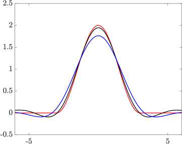
Figure 1: Example 5.1 - Exact solution $x^{\dagger}_{n}$ (red) and approximate solutions $x^{\delta,\ell}_{\alpha,n,i}$ computed by iAT with $i=50$ and $\alpha$ estimated by (R1) (black) and by rule (R2) (blue), for $n=1000$, $\ell=10$ and $\xi=1\%$.

The behavior of the relative error of approximate solutions computed with Algorithm 1 for varying $\alpha$ is displayed in Figure 2. The $\alpha$-values determined by solving equation (R1) or (R2) are marked by “$*$” on the graphs. For a few iterations of the Tikhonov method, i.e. $i=50$, the error computed by the rule (R1) is closer to the minimum with respect to rule (R2).

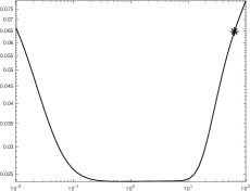
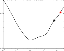
Figure 2: Example 5.1 - Relative error in approximate solutions computed by iAT with $i=50$, when varying $\alpha$ for $n=1000$ and $\xi=1\%$. The point marked by $\ast$ corresponds to the value of $\alpha$ estimated by rule (R1) (black) and by rule (R2) (red). (Left) $\ell=5$, (Right) $\ell=30$.

Example 5.2.

We turn now to the Fredholm integral equation of the first kind discussed by Shaw [22],

$$\int_{-\pi/2}^{\pi/2}\kappa(s,t)x(t)dt=y(s),\qquad-\frac{\pi}{2}\leq s\leq\frac{\pi}{2},$$

where

$$x(t) =a_{1}\exp(-c_{1}(t-t_{1})^{2})+a_{2}\exp(-c_{2}(t-t_{2})^{2}),$$

$$\kappa(s,t) =(\cos(s)+\cos(t))(\sin(y)/y)^{2}\quad\text{and}\quad y(s)=\pi(\sin(s)+\sin(t)).$$

The discretization is computed with the MATLAB function shaw from [11] and gives a nonsymmetric nonsingular matrix $T_{n}\in\mathbb{R}^{n\times n}$ and the vector $x_{n}^{\dagger}\in\mathbb{R}^{n}$.

Table 2 shows the relative error $\|x_{n}^{\dagger}-x_{\alpha,n,i}^{\delta,\ell}\|_{2}/\|x_{n}^{\dagger}\|_{2}$ for several computed approximate solutions $x_{\alpha,n,i}^{\delta,\ell}$ for a noise level given by $\xi=0.1\%$. Note that the rule (R1) computes accurate approximations even for small values of $\ell$ where the rule (R2) fails.

Table 2: Example 5.2 - Relative error in approximate solutions computed by iAT for different values of $\ell$, with $n=1000$ and $\xi=0.1\%$.

			iAT - (R1)			iAT - (R2)
$\ell$	$d_{\ell}$	$i$	$\alpha$	$\|x_{n}^{\dagger}-x_{\alpha,n,i}^{\delta,\ell}\|_{2}/\|x_{n}^{\dagger}\|_{2}$		$\alpha$	$\|x_{n}^{\dagger}-x_{\alpha,n,i}^{\delta,\ell}\|_{2}/\|x_{n}^{\dagger}\|_{2}$
4	$2.01\cdot 10^{-3}$	1	$1.42\cdot 10^{-2}$	$1.76\cdot 10^{-1}$		$2.43\cdot 10^{-1}$	$2.44\cdot 10^{-1}$
		20	$7.97\cdot 10^{-1}$	$1.75\cdot 10^{-1}$		$6.95\cdot 10^{0\phantom{-}}$	$2.26\cdot 10^{-1}$
		40	$1.65\cdot 10^{0\phantom{-}}$	$1.75\cdot 10^{-1}$		$1.41\cdot 10^{1\phantom{-}}$	$2.26\cdot 10^{-1}$
8	$3.01\cdot 10^{-5}$	1	$1.61\cdot 10^{-3}$	$1.05\cdot 10^{-1}$		$1.99\cdot 10^{-3}$	$1.61\cdot 10^{-1}$
		20	$3.01\cdot 10^{-2}$	$9.27\cdot 10^{-2}$		$8.17\cdot 10^{-1}$	$1.64\cdot 10^{-1}$
		40	$6.01\cdot 10^{-2}$	$9.24\cdot 10^{-2}$		$1.68\cdot 10^{0\phantom{-}}$	$1.64\cdot 10^{-1}$
12	$3.87\cdot 10^{-8}$	1	$1.61\cdot 10^{-3}$	$1.05\cdot 10^{-1}$		$1.61\cdot 10^{-3}$	$1.06\cdot 10^{-1}$
		20	$3.00\cdot 10^{-2}$	$9.27\cdot 10^{-2}$		$3.01\cdot 10^{-2}$	$9.27\cdot 10^{-2}$
		40	$6.00\cdot 10^{-2}$	$9.23\cdot 10^{-2}$		$6.01\cdot 10^{-2}$	$9.24\cdot 10^{-2}$

Figure 3 shows the exact solution as well as two approximate solutions computed with iAT with rule (R1) and with rule (R2).

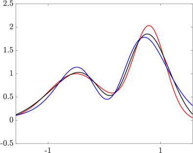
Figure 3: Example 5.2 - Exact solution $x^{\dagger}_{n}$ (red) and approximate solutions $x^{\delta,\ell}_{\alpha,n,i}$ computed by iAT with $i=20$ and $\alpha$ estimated by rule (R1) (black) and by rule (R2) (blue), for $n=1000$, $\ell=8$ and $\xi=0.1\%$.

The behavior of the relative error of approximate solutions computed with Algorithm 1 for varying $\alpha$ is displayed in Figure 4. The $\alpha$-values determined by solving equation (R1) or (R2) are marked by “$*$” on the graphs. Again, we can see that rule (R1) performs substantially better than rule (R2) approaching the minimum.

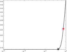
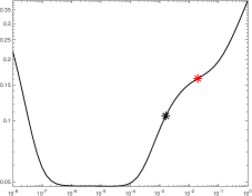
Figure 4: Example 5.2 - Relative error in approximate solutions computed by iAT with $i=20$, when varying $\alpha$ for $n=1000$ and $\xi=0.1\%$. The point marked by $\ast$ corresponds to the value of $\alpha$ estimated by rule (R1) (black) and by rule (R2) (red). (Left) $\ell=4$, (Right) $\ell=8$.

Example 5.3.

This example is concerned with a digital image deblurring problem. We use the function blur from [11] with default parameters to determine an $n^{2}\times n^{2}$ symmetric block Toeplitz nonsingular matrix with Toeplitz blocks, $T_{n^{2}}$, that models blurring of an image that is represented by $n\times n$ pixels. The blur is determined by a space-invariant Gaussian point spread function. The true image is represented by the vector $x_{n^{2}}^{\dagger}\in\mathbb{R}^{n^{2}}$ for $n=30$. This image is shown in Figure 5 with the observed image $y_{n^{2}}^{\delta}$.

Table 3: Example 5.3 - Relative error in approximate solutions computed by iAT for different values of $\ell$, with $n^{2}=900$ and $\xi=1\%$.

			iAT - (R1)			iAT - (R2)
$\ell$	$d_{\ell}$	$i$	$\alpha$	$\|x_{n}^{\dagger}-x_{\alpha,n,i}^{\delta,\ell}\|_{2}/\|x_{n}^{\dagger}\|_{2}$		$\alpha$	$\|x_{n}^{\dagger}-x_{\alpha,n,i}^{\delta,\ell}\|_{2}/\|x_{n}^{\dagger}\|_{2}$
100	$1.36\cdot 10^{-3}$	1	$1.08\cdot 10^{-1}$	$1.17\cdot 10^{-1}$		-	-
		200	$3.01\cdot 10^{0\phantom{-}}$	$1.01\cdot 10^{-1}$		-	-
		500	$2.02\cdot 10^{0\phantom{-}}$	$6.83\cdot 10^{-2}$		-	-
200	$2.69\cdot 10^{-4}$	1	$1.08\cdot 10^{-1}$	$1.17\cdot 10^{-1}$		-	-
		200	$3.01\cdot 10^{0\phantom{-}}$	$1.01\cdot 10^{-1}$		-	-
		500	$2.02\cdot 10^{0\phantom{-}}$	$6.83\cdot 10^{-2}$		-	-
300	$5.13\cdot 10^{-4}$	1	$1.08\cdot 10^{-1}$	$1.17\cdot 10^{-1}$		$2.44\cdot 10^{1}$	$9.72\cdot 10^{-1}$
		200	$3.01\cdot 10^{0\phantom{-}}$	$1.01\cdot 10^{-1}$		$5.82\cdot 10^{0}$	$1.37\cdot 10^{-1}$
		500	$2.02\cdot 10^{0\phantom{-}}$	$6.83\cdot 10^{-2}$		$2.02\cdot 10^{0}$	$6.83\cdot 10^{-2}$

Table 3 displays relative restoration errors for the computed approximate solutions with iAT for a noise level given by $\xi=1\%$. Rule (R1) is satisfied for every value of $\ell$, while rule (R2) requires $\ell\geq 269$. The computed solutions are comparable but the computational cost is much lower for $\ell=100$ compared to $\ell=300$.

Figure 5 depicts the approximate solution computed with iAT with $i=500$ using rule (R1) with $\ell=100$ and using rule (R2) with $\ell=100$.

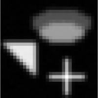
Figure 5: Example 5.3 - Exact solution $x^{\dagger}_{n^{2}}$ (Up-Left), observed image $y_{n^{2}}^{\delta}$ (Up-Right), approximate solutions $x^{\delta,\ell}_{\alpha,n^{2},i}$ computed by iAT with $\ell=100$, $i=500$ and $\alpha$ estimated by rule (R1) (Down-Left) and with $\ell=300$, $i=500$ and $\alpha$ estimated by rule (R2) (Down-Right), for $n^{2}=900$, $\xi=1\%$.

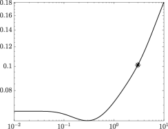
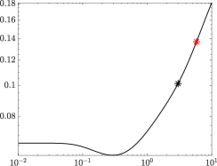
Figure 6: Example 5.3 - Relative error in approximate solutions computed by iAT with $i=200$ varying $\alpha$, for $n^{2}=900$ and $\xi=1\%$. The point marked by $\ast$ correspond to the value of $\alpha$ estimated by rule (R1) (black) and by rule (R2) (red). (Left) $\ell=100$, (Right) $\ell=300$.

Figure 6 displays the relative error of the computed solutions when varying the parameters $\alpha$ for $i=500$. The “$*$” on the graph corresponds to the values of the parameter $\alpha$ determined by solving equations (R1) and (R2).

6 Conclusions

We have introduced a new rule to estimate the regularization parameter of iAT, solving equation (R1). Theoretical analysis, contingent upon further Assumption 4.1, enhances the a posteriori rule presented in [3]. Numerical results confirm the robustness of rule (R1) even for small values of $\ell$, crucial for achieving low computational costs.

References

- [1] P. Alba, L. Fermo, C. Mee and G. Rodriguez “Recovering the electrical conductivity of the soil via a linear integral model” In Journal of Computational and Applied Mathematics 352 Elsevier, 2019, pp. 132–145
- [2] A. H. Bentbib, M. El Guide, K. Jbilou, E. Onunwor and L. Reichel “Solution methods for linear discrete ill-posed problems for color image restoration” In BIT Numerical Mathematics 58 Springer, 2018, pp. 555–578
- [3] Davide Bianchi, Marco Donatelli, Davide Furchi and Lothar Reichel “Convergence analysis and parameter estimation for the iterated Arnoldi-Tikhonov method” arXiv preprint: arXiv:2311.11823 [math.NA] In Submittied for publication, 2024
- [4] C. Boor “A Practical Guide to Splines” Springer, 1978
- [5] Alessandro Buccini, Marco Donatelli and Lothar Reichel “Iterated Tikhonov regularization with a general penalty term” In Numerical Linear Algebra with Applications 24.4, 2017, pp. e2089
- [6] Marco Donatelli “On nondecreasing sequences of regularization parameters for nonstationary iterated Tikhonov” In Numerical Algorithms 60 Springer, 2012, pp. 651–668
- [7] H. W. Engl, M. Hanke and A. Neubauer “Regularization of Inverse Problems” Kluwer, Dordrecht, 1996
- [8] Silvia Gazzola, Paolo Novati and Maria Rosaria Russo “On Krylov projection methods and Tikhonov regularization” In Electronic Transactions on Numerical Analysis 44, 2015, pp. 83–123
- [9] R. W. Goodman “Discrete Fourier and Wavelet Transforms: An Introduction Through Linear Algebra with Applications to Signal Processing” World Scientific Publishing Company, London, 2016
- [10] Martin Hanke and Charles W Groetsch “Nonstationary iterated Tikhonov regularization” In Journal of Optimization Theory and Applications 98 Springer, 1998, pp. 37–53
- [11] Per C. Hansen “Regularization tools version 4.0 for Matlab 7.3” In Numerical Algorithms 46, 2007, pp. 189–194
- [12] Bryan Lewis and Lothar Reichel “Arnoldi-Tikhonov regularization methods” In Journal of Computational and Applied Mathematics 226, 2009, pp. 92–102
- [13] F. Natterer “Regularization of ill-posed problems by projection methods” In Numererische Mathematik 28, 1977, pp. 329–341
- [14] F. Natterer “The Mathematics of Computerized Tomography” SIAM, Philadelphia, 2001
- [15] A. Neubauer “An a posteriori parameter choice for Tikhonov regularization in the presence of modeling error” In Applied Numerical Mathematics 4, 1988, pp. 507–519
- [16] D. L. Phillips “A technique for the numerical solution of certain integral equations of the first kind” In Journal of the ACM 9 ACM, 1962, pp. 84–97
- [17] S. Raffetseder, R. Ramlau and M. Yudytski “Optimal mirror deformation for multi-conjugate adaptive optics systems” In Inverse Problems 32, 2016, pp. 025009
- [18] R. Ramlau and L. Reichel “Error estimates for Arnoldi-Tikhonov regularization for ill-posed operator equations” In Inverse Problems 35, 2019, pp. 055002
- [19] R. Ramlau and M. Rosensteiner “An efficient solution to the atmospheric turbulence tomography problem using Kaczmarz iteration” In Inverse Problems 28 IOP publishing, 2012, pp. 095004
- [20] Y. Saad “Iterative Methods for Sparse Linear Systems” SIAM, Philadelphia, 2003
- [21] O. Scherzer, M. Grasmair, H. Grossauer, M. Haltmeier and F. Lenzen “Variational Methods in Imaging” Springer, New York, 2009
- [22] Jr. C. B. Shaw “Improvements of the resolution of an instrument by numerical solution of an integral equation” In Journal of Mathematical Analysis and Applications 37 Elsevier, 1972, pp. 83–112 DOI: 10.1016/0022-247X(72)90019-5