A splitting, discontinuous Galerkin solver for the cell-by-cell electroneutral Nernst-Planck framework

Abstract

Mathematical models for excitable tissue with explicit representation of individual cells are highly detailed and can, unlike classical homogenized models, represent complex cellular geometries and local membrane variations. However, these cell-based models are challenging to approximate numerically, partly due to their mixed-dimensional nature with unknowns both in the bulk and at the lower-dimensional cellular membranes. We here develop and evaluate a novel solution strategy for the cell-based KNP-EMI model describing ionic electrodiffusion in and between intra- and extracellular compartments with explicit representation of individual cells. The strategy is based on operator splitting, a multiplier-free formulation of the coupled dynamics across sub-regions, and a discontinuous Galerkin discretization. In addition to desirable theoretical properties, such as local mass conservation, the scheme is practical as it requires no specialized functionality in the finite element assembly and order optimal solvers for the resulting linear systems can be realized with black-box algebraic multigrid preconditioners. Numerical investigations show that the proposed solution strategy is accurate, robust with respect to discretization parameters, and that the parallel scalability of the solver is close to optimal – both for idealized and realistic two and three dimensional geometries.

65M60, 65F10, 65M55, 68U20, 92-08, 92C37

1 Introduction

Despite the fundamental role of movements of molecules and ions in and between cellular compartments for brain function [37], most computational models for excitable tissue assume constant ion concentrations [26, 36, 42]. Although these models have provided valuable insight into how neurons function and communicate, they fail to describe vital processes related to ionic signalling and brain homeostasis [34, 12], and pathologies involving substantial changes in the extracellular ion composition such as epilepsy and spreading depression [16, 41, 44]. The emerging KNP-EMI framework [18, 31] is a system of partial differential equations (PDEs) describing the coupling of ion concentration dynamics and electrical properties in excitable tissue with explicit representation of the cells, allowing for morphologically detailed descriptions of the neuropil. In contrast to classical homogenized models, the highly detailed KNP-EMI framework enables modelling of single cells and small collections of cells, uneven distributions of membrane mechanisms, and the role of the cellular morphology in tissue dynamics.

Electrodiffusive transport of each ion species in the intracelluar space (ICS) and extracellular space (ECS) in the KNP-EMI framework is described by a Nernst Planck (NP) equation. To determine the electrical potential in the bulk, the NP equations are coupled with an electroneutrality assumption stating that there is no charge separation anywhere in solution [35, 15]. Consequently, the medium is electroneutral everywhere circumventing the need for resolving charge relaxation processes at the nanoscale. Further, the cellular membranes are explicitly represented as lower-dimensional interfaces separating the intra- and extracellular sub-regions. Coupling conditions at the membrane interface relate the dynamics in the different sub-regions. The resulting problem is mixed-dimensional, containing unknowns in both the intra- and extracellular domains (e.g. electrical potentials) and on the interface/cell membranes (e.g. transmembrane currents). We note that the interface is typically a manifold of co-dimension 1 with respect to the ICS/ECS. Further, the system is non-linear, coupled, and stiff: the fast electrical dynamics and the slow ion diffusion are associated with vastly different time scales. This suggests split solution approaches where the different dynamics are loosely coupled. Nevertheless, the numerical strategies for approximating the system must be chosen with care.

Previously, the KNP-EMI problem has been discretized with a mortar finite element method (FEM), leading to a saddle-point problem where the intra- and extracellular potentials and concentrations are coupled together via Lagrange multipliers on common interfaces [18]. The resulting formulation is challenging for implementation as it necessitates, e.g. support for different finite element spaces on domains/meshes with different topological dimension (ECS, ICS and the membranes) and their coupling. In addition, efficient solvers for the resulting linear systems require specialized multigrid methods [48] or preconditioners [28]. Other discretization approaches for the KNP-EMI model, or its sub-problem the cell-by-cell (EMI) equations [27, 50, 2], have been considered, including, finite volume schemes [31, 49], boundary element methods [39], CutFEM finite element methods [10] or finite differences [45]. Efficient solvers for the different formulations of the EMI model have been developed e.g. in [23, 11, 9, 39].

We here present a novel solution strategy for the KNP-EMI problem where the Lagrange multipliers are eliminated and only the bulk variables are explicitly solved for. As all the problem unknowns are then posed over domains of same topological dimension, we refer to this formulation as single-dimensional. The single-dimensional formulation may be discretized with conforming elements, e.g. continuous Lagrange elements in [8], but several factors motivate us to apply discontinuous Galerkin (DG) schemes instead. In particular, standard DG functionality (e.g. facet integrals) is sufficient to implement to DG schemes for KNP-EMI. This is in contrast to conforming discretization where specialized mixed-mesh coupling across ECS and ICS meshes is required. Moreover, DG methods inherently allow for adaptable refinement and have desirable properties, such as local mass conservation or numerical stability in convection-dominated regime [38]. Our approach further includes an operator splitting technique decoupling the concentrations from the electrical potential reducing the system to two simpler sub-problems: (i) an EMI problem, and (ii) a series of advection diffusion (KNP) problems, which can leverage dedicated, recently developed solvers, e.g. [40, 46, 30].

A key feature of the KNP-EMI models is the ability to handle complex and realistic geometries, often resulting in large-scale systems when discretized. In turn, efficient and scalable solvers are required to utilize the modeling potential of the framework in practical applications. As will become apparent, our splitting approach and DG discretization address these issues as the resulting linear systems are amenable to block-box algebraic multigrid (AMG) preconditioners. Here, the order optimal solvers can thus be realized as AMG-preconditioned Krylov methods.

Through numerical investigations, we demonstrate that our proposed numerical scheme is accurate and yields optimal convergence rates in space and time. In idealised 2D and 3D geometries, we further show that the proposed preconditioners are robust with respect to numerical parameters. Experiments show that the parallel scalability of our solution scheme is close to optimal, enabling large-scale simulations on HPC clusters. Finally, we assess quantities of interest, such as conduction velocity, ECS potentials and concentration shifts in a physiological relevant scenario where we simulate neuronal activity in a morphological realistic 3D geometry representing a pyramidal neuron in the cortex.

2 Mathematical framework

We here present the coupled, time-dependent, non-linear, mixed-dimensional KNP-EMI equations describing ionic electrodiffusion in a geometrically explicit setting. For further details on the derivation of the equations, see e.g. [31, 18].

2.1 Governing equations

We consider $N-1$ domains $\Omega_{i^{n}}\subset\mathbb{R}^{d}$ ($d=1,2,3$) for $n=1,\dots,N-1$ representing disjoint intracellular regions (physiological cells) and an extracellular region $\Omega_{e}$, and let the complete domain be $\Omega=\Omega_{i^{1}}\cup\dots\cup\Omega_{i^{N}}\cup\Omega_{e}$ with boundary $\partial\Omega$. We denote the cell membrane associated with cell $i^{n}$, i.e. the boundary of the physiological cell $\Omega_{i^{n}}$, by $\Gamma_{n}$. We assume that $\Gamma_{n}\cap\Gamma_{m}=\emptyset$ for all $n\not=m$ and that $\Gamma_{n}\cap\partial\Omega=\emptyset$. Below we will denote the restriction of functions $u:\Omega\rightarrow\mathbb{R}$, $f_{l}:\Omega\rightarrow\mathbb{R}$ to $\Omega_{r}$ by $u_{r}$ and $f_{l,r}$ respectively. For notational simplicity and clarity, we present in the following the mathematical model for one intracellular region $\Omega_{i^{1}}=\Omega_{i}$ with membrane $\Gamma$.

We consider a set of ion species $K$. For each ion species $k\in K$, we aim to find the ion concentrations $c_{k}:\Omega\times(0,T]\rightarrow\mathbb{R}$ , the electrical potentials $\phi:\Omega\times(0,T]\rightarrow\mathbb{R}$ and the total transmembrane ion current $I_{M}:\Gamma\times(0,T]\rightarrow\mathbb{R}$ such that:

(1) $$\frac{\partial c_{k}}{\partial t}+\operatorname{\nabla\cdot}\mathbf{J}_{k} =0 \qquad\text{in }\Omega,$$

(2) $$F\sum_{k\in K}z_{k}\operatorname{\nabla\cdot}\mathbf{J}_{k} =0 \qquad\text{in }\Omega,$$

(3) $$\phi_{M} =\phi_{i}-\phi_{e} \qquad\text{ on }\Gamma,$$

(4) $$I_{M}\equiv-F\sum_{k\in K}z_{k}\mathbf{J}_{k,e}\cdot\mathbf{n}_{e} =F\sum_{k\in K}z_{k}\mathbf{J}_{k,i}\cdot\mathbf{n}_{i} \qquad\text{ on }\Gamma,$$

(5) $$\mathbf{J}_{k,i}\cdot\mathbf{n}_{i} =\frac{I_{\text{ch},k}+\alpha_{k,i}(I_{M}-I_{\text{ch}})}{Fz_{k}} \qquad\text{ on }\Gamma,$$

(6) $$-\mathbf{J}_{k,e}\cdot\mathbf{n}_{e} =\frac{I_{\text{ch},k}+\alpha_{k,e}(I_{M}-I_{\text{ch}})}{Fz_{k}} \qquad\text{ on }\Gamma,$$

(7) $$\frac{\partial\phi_{M}}{\partial t} =\frac{1}{C_{M}}(I_{M}-I_{\text{ch}}) \qquad\text{ on }\Gamma,$$

where each regional ion flux density $\mathbf{J}_{k}:\Omega\times(0,T]\rightarrow\mathbb{R}^{d}$ can be expressed by a Nernst-Planck equation as follows:

(8) $$\mathbf{J}_{k}=-D_{k}\nabla c_{k}-c_{k}z_{k}D_{k}\psi\nabla\phi,\qquad\text{in }\Omega$$

stating that ionic movement is driven by both diffusion due to ionic gradients (first term) and drift in the electrical field (second term). Note that the drift term may be interpreted as an advective term where $z_{k}D_{k}\psi\nabla\phi$ drives the advection. The constant $\psi=F/(RT)$ combines the effective diffusion coefficient $D_{k}$, Faraday’s constant $F$, the absolute temperature $T$, and the gas constant $R$. Further the membrane capacitance, the valence and the diffusion coefficient for ion species $k$ are denoted by $C_{M}$, $z_{k}$ and $D_{k}$, respectively. In the coupling conditions (5)–(6), we assume that the ion specific capacitive current is some fraction $\alpha_{k}:\Gamma\times(0,T]\rightarrow\mathbb{R}$ of the total capacitive current where

(9) $$\alpha_{k}=\frac{D_{k}z_{k}^{2}c_{k}}{\sum_{l\in K}D_{l}z_{l}^{2}c_{l}}\qquad\text{ on }\Gamma.$$

The ion specific channel currents are denoted by $I_{\text{ch},k}:\Gamma\times(0,T]\rightarrow\mathbb{R}$ and will depend on the membrane potential $\phi_{M}:\Gamma\times(0,T]\rightarrow\mathbb{R}$ and typically be of the form

(10) $$I_{\text{ch},k}=g_{k}(\phi_{M}-E_{k}),\qquad E_{k}=\frac{RT}{z_{k}F}\ln{\frac{c_{k,e}}{c_{k,i}}}\qquad\text{ on }\Gamma,$$

where $g_{k}$ and $E_{k}$ denotes respectively the channel conductance and the Nernst potential for ion species $k$. The total ion current $I_{\text{ch}}:\Gamma\times(0,T]\rightarrow\mathbb{R}$ is given by $I_{\text{ch}}=\sum_{k}I_{\text{ch},k}$. In many physiological scenarios, the ion specific currents $I_{\text{ch},k}$ will further depend on gating variables $\mathbf{s}:\Gamma\times(0,T]\rightarrow\mathbb{R}^{S}$, where $S$ is the number of gating variables, governed by ordinary differential equations (ODEs) of the following form:

(11) $$\frac{\partial\phi_{M}}{\partial t}=\frac{1}{C_{M}}(I_{M}-I_{\text{ch}})\qquad\text{ on }\Gamma,$$

(12) $$\frac{\partial\mathbf{s}}{\partial t}=F(\phi_{M},\mathbf{s})\qquad\text{ on }\Gamma.$$

We will refer to membrane models depending on variables governed by ODEs as active.

2.2 Formulation with fewer concentrations

The equation for the electrical potential (2) is derived assuming electroneutrality (see e.g. [31, 40] for further details). The electroneutrality assumption states that there is no charge separation in the bulk, and that the bulk of the tissue is electroneutral:

(13) $$0=\sum_{k=1}^{K}z_{k}c_{k}\qquad\text{in }\Omega.$$

Using (13), we can express one of the ion concentrations as:

(14) $$c_{m}=-\frac{1}{z_{m}}\sum_{k=1}^{m-1}z_{k}c_{k}\qquad\text{in }\Omega.$$

By inserting  (14) into (2) and (4), we can eliminate $c_{m}$ from the system. Let $\tilde{K}$ be $K\setminus\{m\}$. The modified system reads: for each $k\in\tilde{K}$, find the ion concentrations $c_{k}:\Omega\times(0,T]\rightarrow\mathbb{R}$, the electrical potentials $\phi:\Omega\times(0,T]\rightarrow\mathbb{R}$ and the total transmembrane ion current $I_{M}:\Gamma\times(0,T]\rightarrow\mathbb{R}$ such that (1)–(7) hold. The eliminated concentration $c_{m}$ can be recovered via (14).

2.3 Boundary and initial conditions

The system must be closed by appropriate initial and boundary conditions. We assume that initial conditions are given for the ion concentrations $c_{k}=c_{k}(\mathbf{x},t)$ for $k\in K$ and for the membrane potential $\phi_{M}=\phi_{M}(\mathbf{x},t)$:

(15) $$\begin{split}c_{k}(\mathbf{x},0)&=c_{k}^{0}=\begin{cases}c_{k,i}^{0}&\quad\text{if }\mathbf{x}\in\Omega_{i}\\ c_{k,e}^{0}&\quad\text{if }\mathbf{x}\in\Omega_{e},\end{cases}\end{split}$$

(16) $$\phi_{M}(\mathbf{x},0) =\phi_{M}^{0}\qquad\qquad\quad\quad\mathbf{x}\in\Gamma,$$

where the initial concentrations $c_{k}^{0}$ satisfy the electroneutrality assumption, i.e.:

(17) $$0=\sum_{k=1}^{K}z_{k}c_{k}^{0}\qquad\text{in }\Omega.$$

Finally, we state that no ions can leave or enter the system by imposing the following Neumann boundary condition for $k\in K$:

(18) $$\mathbf{J}_{k}(\mathbf{x},t)\cdot\mathbf{n}=0\qquad\mathbf{x}\in\partial\Omega.$$

We note with (18) the electrical potential in (1)-(7) is determined only up to a constant.

3 Numerical scheme

We here consider a single-dimensional formulation of the KNP-EMI equations where the total transmembrane ion current variable $I_{M}$ is eliminated. Our approach is further based on a decoupling of the Nernst-Planck equations (1) for ionic transport and equation (2) governing the electrical potential, as well an operator splitting scheme to decouple the ODEs from the PDEs. For spatial discretization we will finally employ the DG finite element method.

3.1 Temporal discretization and splitting scheme

We start by discretizing the system in time. For each time step $t^{n}$, we assume that the concentrations $c_{k}^{n-1}$ and the membrane potential $\phi_{M}^{n-1}$ are known for $t^{n-1}$. The time derivatives in (1) and (7) are approximated respectively by

(19) $$\frac{\partial c_{k}}{\partial t}\approx\frac{c_{k}^{n}-c_{k}^{n-1}}{\Delta t}\quad\text{and}\quad\frac{\partial\phi_{M}}{\partial t}\approx\frac{\phi_{M}^{n}-\phi_{M}^{n-1}}{\Delta t}$$

with step size $\Delta t$. To solve (1) and (2) at time $t^{n}$, we apply the following two step splitting scheme where $c_{k}^{n}$ and $\phi^{n}$ denote respectively the ion concentrations and electrical potential at $t^{n}$:

• Find $\phi^{n}$ such that:

  (20) $$F\sum_{k\in K}z_{k}\operatorname{\nabla\cdot}{\mathbf{J}_{k}^{n}} =0,$$

  (21) $${\mathbf{J}_{k}^{n}} =-D_{k}\nabla c_{k}^{n-1}-z_{k}D_{k}\psi c_{k}^{n-1}\nabla\phi^{n}.$$

• Find $c_{k}^{n}$ such that:

  (22) $${\Delta t}^{-1}c_{k}^{n}+\operatorname{\nabla\cdot}\mathbf{J}_{k}^{n} ={\Delta t}^{-1}c_{k}^{n-1},$$

  (23) $$\mathbf{J}_{k}^{n} =-D_{k}\nabla c_{k}^{n}-z_{k}D_{k}\psi c_{k}^{n}\nabla\phi^{n}$$

  for $k\in\tilde{K}$. Update $c_{k}^{n-1}=c_{k}^{n}$ and $\phi_{M}^{n-1}=\phi^{n}_{i}-\phi^{n}_{e}$.

In both steps, the Neumann boundary conditions (18) are assumed. Consequently, the first problem determining the electrical potential $\phi^{n}$ is singular with constants in the nullspace. Moreover, its solvability requires that the right-hand-side in (20)-(21) satisfies certain compatibility condition. This point will be made more specific when we discuss linear solvers in Section 4.

Next, we eliminate the unknown total transmembrane ion current $I_{M}$ via the temporal discretization of (7) to obtain a single-dimensional form. The time derivative in (7) is approximated by (19) and the coefficients $\alpha_{k}$, the Nernst potentials $E_{k}$, and the ionic currents $I_{\text{ch},k}$ are treated explicitly:

$$\alpha_{k} \approx\alpha_{k}^{n-1}=\frac{D_{k}z_{k}^{2}c_{k}^{n-1}}{\sum_{l\in K}D_{l}z_{l}^{2}c_{l}^{n-1}},\qquad E_{k}\approx E_{k}^{n-1}=\frac{RT}{z_{k}F}\ln{\frac{c_{k,e}^{n-1}}{c_{k,i}^{n-1}}},$$

$$I_{\text{ch},k} \approx I_{\text{ch},k}^{n-1}=I_{\text{ch},k}(\phi_{M}^{n-1},c_{k}^{n-1}).$$

For notational simplicity, we omit the temporal superscript and denote $\alpha^{n-1}_{k}$ by $\alpha_{k}$, $E_{k}^{n-1}$ by $E_{k}$, and $I_{\text{ch},k}^{n-1}$ by $I_{\text{ch},k}$ below. Similar convention will be applied also to other variables. By inserting (3) into the discrete counterpart of (7) we obtain the following expression for the total transmembrane ion current $I_{M}$:

(24) $$I_{M}=\frac{C_{M}}{\Delta t}(\phi_{i}^{n}-\phi_{e}^{n}-f)\qquad\text{ on }\Gamma,$$

where

(25) $$f=f^{n-1}=\phi_{M}^{n-1}-\frac{\Delta t}{C_{M}}I_{\text{ch}}.$$

We observe that (24) represents a Robin-type interface condition for $\phi^{n}_{i}$ and $\phi^{n}_{e}$. Specifically, by inserting (24) into (5) and (6) we get the following new expression for the ion specific fluxes across the cellular membrane interface:

(26) $$\mathbf{J}_{k,i}\cdot\mathbf{n}_{i}=\frac{\alpha_{k,i}C_{M}}{Fz_{k}\Delta t}(\phi_{i}^{n}-\phi_{e}^{n}-g_{k,i})\qquad\text{ on }\Gamma,$$

(27) $$-\mathbf{J}_{k,e}\cdot\mathbf{n}_{e}=\frac{\alpha_{k,e}C_{M}}{Fz_{k}\Delta t}(\phi_{i}^{n}-\phi_{e}^{n}-g_{k,e})\qquad\text{ on }\Gamma,$$

where $g_{k,i}$ and $g_{k,e}$ denote the restrictions of $g_{k}$ to respectively $\Omega_{i}$ and $\Omega_{e}$ with

(28) $$g_{k}=g_{k}^{n-1}=\phi_{M}^{n-1}-\frac{\Delta t}{C_{M}\alpha_{k}}.$$

Note that in the case of an active membrane model (governed by ODEs) the expressions for $f$ and $g_{k}$ will change, as we shall see later in Section 3.3.

3.2 Spatial discretization

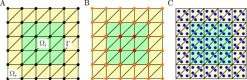
Figure 1: Finite element discretization of the KNP-EMI model by continuous linear and discontinuous linear Lagrange elements. Setup with single intracellular domain $\Omega_{i}$ (in green) is considered. Triangulation conforms to the interface $\Gamma$. Mesh vertices are shown with black circle markers (A). Intra-/extracellular variables are represented in separate $H^{1}$-conforming FE spaces over different meshes of $\Omega_{i}$ and $\Omega_{e}$. The coupling requires specialized implementation as on $\Gamma$ the degrees of freedom (shown with red and orange markers) interact (B). With DG discretization the problem unknowns are represented in a single FE spaces posed over the global mesh. Coupling on $\Gamma$ requires no special treatment compared to the remaining facets. However, the scheme leads to more degrees of freedom (shown in blue markers, C).

To derive the DG discretizations of KNP-EMI sub-problems let us first consider their continuous variational formulations. To this end, and to simplify the exposition, we shall keep the assumption of only a single intracellular domain. We then let $L^{2}(\Omega_{r})$, $r\in\left\{e,i\right\}$ be the Lebesque space of square-integrable functions while $H^{1}(\Omega_{r})$ is the standard Sobolev space of functions with derivatives up to order one in $L^{2}(\Omega_{r})$. For $u=(u_{i},u_{e})\in V$ let us finally define a membrane jump

(29) $$[u]_{m}=u_{i}|_{\Gamma}-u_{e}|_{\Gamma}.$$

From the trace theorem in then follows that $[u]_{m}\in L^{2}(\Gamma)$ for all $u\in V$, see e.g. [1].

3.2.1 Continuous problems

Multiplying the EMI sub-problem (20)–(21) with a suitable test function $w\in V$, integrating over each sub-domain $\Omega_{r}$ for $r\in\{i,e\}$, performing integration by parts, summing over the sub-domains, and inserting interface condition (24) yield the following weak form: Given $c_{k}^{n-1}\in V$ and $\phi_{M}^{n-1}\in L^{2}(\Gamma)$ at time level $n-1$, find the electrical potential $\phi^{n}\in V$ at time level $n$ such that:

(30) $$a_{\phi}(\phi^{n},w)=l_{\phi}(w)\quad\forall w\in V,$$

where

$$a_{\phi}(\phi^{n},w) =\sum_{r\in\{i,e\}}\int_{\Omega_{r}}\kappa\nabla\phi^{n}\cdot\nabla w+C\int_{\Gamma_{m}}[\phi^{n}]_{m}[w]_{m},$$

$$l_{\phi}(w)= -\sum_{r\in\{i,e\}}\int_{\Omega_{r}}\sum_{k\in{K}}z_{k}(D_{k})\nabla c_{k}^{n-1}\cdot\operatorname{\nabla}w+C\int_{\Gamma_{m}}f[w]_{m}$$

$$+F\int_{\partial\Omega}\sum_{k\in{K}}z_{k}{\mathbf{J}_{k}^{n}}\cdot\mathbf{n}w$$

with $\kappa=\kappa^{n-1}=F\sum_{k\in{K}}z_{k}^{2}D_{k}\psi c_{k}^{n-1}$ and interface data $C=\frac{C_{M}}{\Delta t}$ and $f$ given by (25) in the case of a passive membrane model or (35) in the case of an active membrane model (cf. Section 3.3). We observe that $a_{\phi}$ is invariant to the ordering/sign in definition of the jump operator (29).

Similarly, we obtain the following weak form of the KNP sub-problem by multiplying (22)–(23) with a suitable test function, integrating over each sub-domain $\Omega_{r}$ for $r\in\{i,e\}$, integration by parts, summing over the sub-domains, and inserting interface conditions (26)–(27): Given $\phi^{n}\in V$ at time level $n$, for each $k\in\tilde{K}$ find the concentrations $c_{k}^{n}\in V$ at time level $n$ such that:

(31) $$\frac{1}{\Delta t}\int_{\Omega}c_{k}^{n}v_{k}+a_{c_{k}}(c_{k}^{n},v_{k})=\frac{1}{\Delta t}\int_{\Omega}c_{k}^{n-1}v_{k}+l_{c_{k}}(v_{k})\quad\forall v_{k}\in V,$$

where

$$\begin{split}a_{c_{k}}(c_{k}^{n},v_{k})&=\sum_{r\in\{i,e\}}\int_{\Omega_{r}}(D_{k}\nabla c_{k}^{n}\cdot\nabla v_{k}+z_{k}\psi D_{k}c_{k}^{n}\nabla\phi_{r}^{n}\cdot\nabla v_{k}),\end{split}$$

$$\begin{split}l_{c_{k}}(v_{k})=&-\int_{\Gamma_{m}}(([C_{k}]_{m}\{v_{k}\}+\{C_{k}\}[v_{k}]_{m})[\phi]_{m}-[C_{k}g_{k}v_{k}]_{m})-\int_{\partial\Omega}(\mathbf{J}_{k}\cdot\mathbf{n})v_{k}\end{split}$$

with interface data $C_{k}=C_{k}^{n-1}=\frac{\alpha_{k}C_{M}}{Fz_{k}\Delta t}$ and $g_{k}$ given by (28) in the case of a passive membrane model or by (36) in the case of active membrane mechanism governed by ODEs (cf. Section 3.3).

3.2.2 DG discretization

Let $\mathcal{T}^{h}$ be a triangulation of $\Omega$ which conforms to the interface $\Gamma$ in the sense that for any element $E\in\mathcal{T}^{h}$ the intersection of $\Gamma$ with $\partial E$ is either a vertex or an entire face of the element (or an entire edge if $d=3$), cf. Figure 1. Here $h>0$ represents a characteristic mesh size. We let $\mathcal{F}^{h}$ be the collections of all facets of $\mathcal{T}^{h}$ and $\mathcal{F}^{h}_{m}=\Gamma\cap\mathcal{F}^{h}$, $\mathcal{F}^{h}_{e}=\partial\Omega\cap\mathcal{F}^{h}$, $\mathcal{F}^{h}_{i}=\mathcal{F}^{h}\setminus(\mathcal{F}^{h}_{m}\cup\mathcal{F}^{h}_{e})$ shall be respectively, the membrane, exterior and (non-membrane) interior facets.

With the conforming mesh the continuous weak formulations (30) and (31) can be readily discretized by $H^{1}$-conforming elements (e.g, continuous Lagrange elements), posed on meshes $\mathcal{T}^{h}\cap\Omega_{r}$, see [23, 9]. We note that non-conforming meshes can be handled by CutFEM techniques [10]. Here, discretization by DG elements shall be pursued.

The discrete approximations of (30) and (31) are obtained by applying standard DG techniques to handle the operators in the sub-domains’ interiors. In particular, the interface terms on $\Gamma$ will remain unchanged from the continuous problem. Given the polynomial degree $p\geq 1$, let $\mathbb{P}_{p}(E)$ be the space of polynomials of degrees up to $p$ on $E$. We denote by $V^{h}_{p}$ the space of functions in $L^{2}(\mathcal{T}^{h})$ whose restriction to each element $E$ is in $\mathbb{P}_{p}(E)$. For $u\in V^{h}_{p}$ and any facet $e\in\mathcal{F}^{h}$ shared by elements $E_{1}$ and $E_{2}$ we define respectively the jump and average operators

(32) $$[u]=u_{1}-u_{2},\quad\{u\}=\frac{u_{1}+u_{2}}{2}\quad\text{on }e\in\mathcal{F}_{i}^{h}\cup\mathcal{F}^{h}_{m},$$

where $u_{1}=:u|_{E_{1}}$ and $u_{2}=:u|_{E_{2}}$. Note that the jump operator (32) extends the membrane jump (29) to all the interior facets.

Applying the symmetric interior penalty method on the diffusive term with respect to the unknown $\phi$ and with a penalty parameter $\beta>0$ (see e.g. [6] or [38]), the discrete weak form of (30) reads: Given $c_{k}^{n-1}\in V^{h}_{p}$ and $\phi_{M}^{n-1}\in L^{2}(\Gamma)$ at time level $n-1$, find the electrical potential $\phi\in V^{h}_{p}$ at time level $n$ such that:

(33) $$a_{\phi}^{h}(\phi^{n},w)=l^{h}_{\phi}(w)\quad\forall w\in V^{h}_{p},$$

where

$$a_{\phi}^{h}(\phi^{n},w) =\sum_{E\in\mathcal{T}^{h}}\int_{E}\kappa\nabla\phi^{n}\cdot\nabla w+C\sum_{e\in\mathcal{F}_{i}^{h}}\int_{e}[\phi^{n}][w]$$

$$-\sum_{e\in\mathcal{F}_{m}^{h}}\int_{\Gamma_{e}}(\{\kappa\nabla\phi^{n}\cdot\mathbf{n}_{e}\}[w]+\{\kappa\nabla w\cdot\mathbf{n}_{e}\}[\phi^{n}]-\frac{\beta}{h_{f}}\kappa[\phi^{n}][w]),$$

and

$$l_{\phi}^{h}(w)= -\sum_{E\in\mathcal{T}^{h}}F\int_{E}\sum_{k\in{K}}z^{k}D_{k}\nabla c_{k}^{n-1}\cdot\nabla w+F\sum_{e\in\mathcal{F}_{i}^{h}}\int_{e}\sum_{k\in{K}}z_{k}\{D_{k}\nabla c_{k}^{n-1}\cdot\mathbf{n}_{e}\}[w]$$

$$+C\sum_{e\in\mathcal{F}_{m}^{h}}\int_{e}f[w]+F\sum_{e\in\mathcal{F}_{e}^{h}}\int_{e}\sum_{k\in{K}}z^{k}({\mathbf{J}_{k}^{n}}\cdot\mathbf{n}_{e})w$$

with interface data $C=\frac{C_{M}}{\Delta t}$ and $f$ given by (25). We remark that $\beta>0$ needs to be chosen large enough such that (33) is positive definite. Furthermore, we note that the definition/sign in the jump operator (32) does not alter the bilinear form $a_{\phi}^{h}$. However, for consistency of $l^{h}_{\phi}$ (with $l_{\phi}$ in (30)) we require that the operator is consistent with the membrane jump $[\cdot]_{m}$ (29) on $\mathcal{F}^{h}_{m}$.

Similarly, we consider the following discrete approximation of (22)–(23): Given $\phi^{n}\in V^{h}_{p}$ at time level $n$, for each $k\in\tilde{K}$ find the concentrations $c_{k}^{n}\in V^{h}_{p}$ at time level $n$ such that:

(34) $$\sum_{E\in\mathcal{T}_{h}}\frac{1}{\Delta t}\int_{E}c_{k}^{n}v_{k}+a_{c_{k}}^{h}(c_{k}^{n},v_{k})=\sum_{E\in\mathcal{T}_{h}}\frac{1}{\Delta t}\int_{E}c_{k}^{n-1}v_{k}+l_{c_{k}}^{h}(v_{k})\quad\forall v_{k}\in V^{h}_{p},$$

where

$$\begin{split}a_{c_{k}}^{h}(c_{k}^{n},v_{k})&=\sum_{E\in\mathcal{T}_{h}}\int_{E}\bigl{(}D_{k}\nabla c_{k}^{n}\cdot\nabla v_{k}+z_{k}\psi D_{k}c_{k}^{n}\nabla\phi_{r}\cdot\nabla v_{k}\bigr{)}\\ &-\sum_{e\in\mathcal{F}_{i}^{h}}\int_{e}(\{D_{k}\nabla c_{k}^{n}\cdot\mathbf{n}_{e}\}[v_{k}]+\{D_{k}\nabla v_{k}\cdot\mathbf{n}_{e}\}[c_{k}^{n}]-\frac{\gamma}{h_{f}}D_{k}[c_{k}^{n}][v_{k}])\\ &-z_{k}\psi\sum_{e\in\mathcal{F}_{i}^{h}}\int_{e}(\{D_{k}c_{k}^{n}\nabla\phi\}-\frac{|D_{k}\nabla\phi\cdot\mathbf{n}_{e}|}{2}[c_{k}^{n}])[v_{k}],\end{split}$$

$$\begin{split}l_{c_{k}}^{h}(v_{k})=&-\sum_{e\in\mathcal{F}_{m}^{h}}\int_{e}(([C_{k}]\{v_{k}\}+\{C_{k}\}[v_{k}])[\phi]-[C_{k}g_{k}v_{k}])-\sum_{e\in\mathcal{F}_{e}^{h}}\int_{e}(\mathbf{J}_{k}\cdot\mathbf{n})v_{k}\end{split}$$

with interface data $C_{k}=C_{k}^{n-1}=\frac{\alpha_{k}C_{M}}{Fz_{k}\Delta t}$ and $g_{k}$ given by (28). Here, we have applied a symmetric interior penalty method on the diffusive term with penalty parameter $\gamma$, and the advective term is up-winded (see e.g. [6] or [38]). The weak form (31) is obtained by multiplying (22) with a suitable test function $v_{k}\in V_{p}^{h}$, integrating over one element $E\in\mathcal{T}_{h}$, integration by parts on both the diffusive term and the advective term, summing over all elements $E\in\mathcal{T}_{h}$, and inserting interface conditions (26)–(27) in the integral over $\Gamma_{m}$.

3.3 Extension of scheme for active (ODE governed) membrane models

In the active case, where the total ionic current $I_{\text{ch}}=I_{\text{ch}}(\phi_{M},\mathbf{s})$ depends on the membrane potential $\phi_{M}$ and gating variables $\mathbf{s}$ governed by ODEs of the form (11)–(12), we add an additional first order Godunov splitting step (see e.g. [43]) to the splitting scheme presented in Section 3.1. In the first step, we update the membrane potential $\phi_{M}^{n}$ at time step $t^{n}$ by solving the ODE system (12)–(11) with $I_{M}$ set to zero, using a suitable ODE solver with time step $\Delta t^{\ast}$. In the second step, we solve for $\phi^{n}$ and $c_{k}^{n}$ in (20)–(23) (i.e. solve step I and II) with $I_{\text{ch}}$ set to zero in interface condition (24). This results in the following new expression

(35) $$f=f^{n-1}=\phi_{M}^{n-1}$$

replacing (25). Setting $I_{\text{ch}}$ to zero in (24) will further affect the interface conditions (26), and (27). Specifically, we obtain the following new expression

(36) $$g_{k}=g_{k}^{n-1}=\phi_{M}^{n-1}-\frac{\Delta t}{C_{M}\alpha_{k}}I_{\text{ch},k}+\frac{\Delta t}{C_{M}}I_{\text{ch}}$$

replacing (28). An outline of the complete solution algorithm, for the case with an active membrane model, can be found in Algorithm 1.

Algorithm 1 Solution algorithm for the KNP-EMI system with active membrane

set $c_{k}^{0}$ for $k\in\tilde{K}$ and $\phi_{M}^{0}$

for $n=1,\dots,N$ do

     set $\phi_{M}^{m-1}=\phi_{M}^{n-1}$ and solve ODEs:

     for $m=1,\dots,M$ do

         solve ODEs

         $\phi_{M}^{m-1}\leftarrow\phi_{M}^{m}$

     end for

     set $\phi_{M}^{n-1}=\phi_{M}^{m}$ and solve PDEs:

     find $\phi^{n}$ by solving (33) with interface data (35)

     find $c_{k}^{n}$ for $k\in\tilde{K}$ by solving (34) with interface data (36)

     $\phi_{M}^{n-1}\leftarrow(\phi_{i}^{n}-\phi_{e}^{n})$

     $c_{k}^{n-1}\leftarrow c_{k}^{n}$ for $k\in\tilde{K}$ (and thus updating $\alpha_{k},E_{k},I_{\text{ch},k}$ and $\kappa$)

end for

4 Solvers

The numerical scheme presented in Section 3 results in an algorithm where three discrete sub-problems must be solved: (i) an EMI problem governing the electrical potentials, (ii) a series of advection diffusion (KNP) problems governing ion transport, and (iii) a system of ODEs defined on the mesh facts representing the lower dimensional (membrane) interfaces between the sub-regions.

EMI sub-problem

The DG discretization (33) of EMI problem leads to a linear system $A_{\phi}x_{\phi}=b_{\phi}$ for the expansion coefficients $x_{\phi}\in\mathbb{R}^{m}$ of the unknown potential $\phi^{n}$ with respect to the basis of $V^{h}_{p}$, $\text{dim}V^{h}_{p}=m$. As noted earlier, for sufficiently large stabilization parameter $\beta$ the problem matrix $A_{\phi}$ is positive semi-definite with vector $z_{\phi}=1$ in the kernel, i.e. $A_{\phi}z_{\phi}=0$. Solvability of the linear system then requires that $b_{\phi}$ is orthogonal (in the $l^{2}$ inner product) to the kernel. For such compatible $b_{\phi}$, unique solution can be obtained in the orthogonal complement of $R^{m}$ with respect to $z_{\phi}$.

Due to symmetry and positivity of $A_{\phi}$, and following orthogonalization of $b_{\phi}$, the unique $x_{\phi}$ can be obtained by conjugate gradient (CG) method informed about the nullspace, see e.g. [24]. To accelerate convergence of the Krylov solver we will consider a preconditioner realized as a single V-cycle of algebraic multigrid (AMG)[19] applied to the positive definite matrix $P_{\phi}=A_{\phi}+\alpha M$ where $M$ is the mass matrix of $V^{h}_{p}$ and $\alpha>0$ is a scaling parameter dependent on the domain. We remark that, theoretical analysis of AMG for the EMI sub-problem is an active area of research. In particular, using conforming FEM discretizations [11] prove uniform convergence of aggregation-based AMG with custom smoothers to handle the interface. However, with DG discretization, assuming that $\Delta t$ scales at most linearly in $h$, the interface $\Gamma$ (or $\mathcal{F}^{h}_{m}$) does not present additional challenge compared to the remaining facet couplings on $\mathcal{F}^{h}_{i}$. Therefore, existing AMG algorithms for elliptic problems, e.g. [5] and references therein, could be applied.

KNP sub-problem

The discrete KNP sub-problem (34) yields a linear system $A_{c}x_{c}=b_{c}$. Here, the lower-order term stemming from temporal discretization ensures that the matrix $A_{c}$ is positive-definite. Since the problem is not symmetric we apply generalized minimal residual method (GMRes) using single AMG[19] V-cycle applied to $A_{c}$ as the preconditioner.

ODE solver

For the ODE step in our splitting algorithm we apply the LSODA method [20] from ODEPACK [21].

5 Simulation scenarios and parameters

In this section, we define five simulations scenarios, with increasing complexity and physiological relevance, that will be used to numerically investigate the discretization scheme and solvers presented in respectively Section 3 and 4. We always consider three ion species, namely potassium ($\rm K^{+}$), sodium ($\rm Na^{+}$) and chloride ($\rm Cl^{-}$), and model parameters and initial data given in Table 1 unless otherwise stated in the text.

Parameter	Value	Parameter	Value
$R$	8.314 J/(K mol)	$c_{\text{Na},i}^{0}$	12 mM
$T$	300 K	$c_{\text{Na},e}^{0}$	100 mM
$F$	$9.648\cdot 10^{4}$ C/mol	$c_{\text{K},i}^{0}$	125 mM
$C_{M}$	$0.01$ F/m	$c_{\text{K},e}^{0}$	4 mM
$D^{\text{Na}}_{r}$	$1.33\cdot 10^{-9}$ m2/s	$c_{\text{Cl},i}^{0}$	137 mM
$D^{\text{K}}_{r}$	$1.96\cdot 10^{-9}$ m2/s	$c_{\text{Cl},e}^{0}$	104 mM
$D^{\text{Cl}}_{r}$	$2.03\times 10^{-9}$ m2/s	$\phi_{M}^{0}$	$-67.74\times 10^{-3}$ V
$g_{\text{leak,Na}}$	1.0 S/m2	$\Delta t$	$1.0\times 10^{-4}$ s
$g_{\text{leak,K}}$	4.0 S/m2	$\Delta t^{\ast}$	$1.0\times 10^{-4}$ s
$g_{\rm syn}$	40 S/m2	$\beta,\gamma$	$20\times d\times p$
$\tau$	$0.02$ s

Table 1: Physical and numerical parameters and initial values used in the simulations. All units are reported in SI base units. The Hodgkin-Huxley parameters are taken from [18]. The penalty parameter $\beta$ arising from the DG discretization depends on the geometrical dimension (d) and the polynomial degree of the element (p). The ODE solver in our implementation is adaptive with respect to the timestep, and $\Delta t^{\ast}$ is the maximum ODE timestep.

5.1 Model A: Smooth manufactured solutions

To evaluate the numerical accuracy of the discretization scheme presented in Section 3, we construct two analytical solutions using the method of manufactured solutions: one that is constant in time ((37), to assess spatial accuracy), and one that is linear in space ((38), to assess temporal accuracy). In both cases, we consider a two-dimensional domain $\Omega=\Omega_{i}\cup\Omega_{e}=[0,1]\times[0,1]$, with one intracellular sub-domain $\Omega_{i}=[0.25,0.75]\times[0.25,0.75]$. To assess the numerical errors from the spatial discretization scheme, we let the analytical solutions to (1)–(2) be given by:

(37) $$c_{\textrm{Na},i} =0.7+0.3\sin(2\pi x)\sin(2\pi y) \qquad\text{in }\Omega_{i},$$

$$c_{\textrm{Cl},i} =0.3+0.4\cos(2\pi x)\sin(2\pi y) \qquad\text{in }\Omega_{i},$$

$$\phi_{i} =\cos(2\pi x)\cos(2\pi y) \qquad\text{in }\Omega_{i},$$

$$c_{\textrm{Na},e} =0.7+0.2\cos(2\pi x)\cos(2\pi y) \qquad\text{in }\Omega_{e},$$

$$c_{\textrm{Cl},e} =0.3+0.8\sin(2\pi x)\cos(2\pi y) \qquad\text{in }\Omega_{e},$$

$$\phi_{e} =\sin(2\pi x)\sin(2\pi y) \qquad\text{in }\Omega_{e}.$$

We then obtain a series of uniformly refined meshes of the domain by first subdividing $\Omega$ into $n\times m$ rectangles each of which is then split into two triangles. We let $n=m\in\left\{16,32,64,128,256\right\}$. We further let $\Delta t=1\times 10^{-10}$ and evaluate the errors at $t=2\times 10^{-10}$. To assess the numerical errors from the temporal discretization and PDE splitting scheme, we let the analytical solutions to (1)–(2) be given by:

(38) $$c_{\textrm{Na},i} =1+x+y+0.3\cos(2\pi t) \qquad\text{in }\Omega_{i},$$

$$c_{\textrm{Cl},i} =1+x+y+0.2\cos(2\pi t) \qquad\text{in }\Omega_{i},$$

$$\phi_{i} =1+x+y \qquad\text{in }\Omega_{i},$$

$$c_{\textrm{Na},e} =1+x+y+0.5\sin(2\pi t) \qquad\text{in }\Omega_{e},$$

$$c_{\textrm{Cl},e} =1+x+y+0.6\sin(2\pi t) \qquad\text{in }\Omega_{e},$$

$$\phi_{e} =1+x+y \qquad\text{in }\Omega_{e}.$$

We mesh the domain with $n=m=64$ and consider first order DG elements. We initially let $\Delta t=1\times 10^{-6}$ and half the time step on refinement. The errors are evaluated at $t=2\times 10^{-6}$.

5.2 Model B: Idealized 2D axon with active membrane model

We next consider a model scenario with active membrane mechanisms depending on gating variables governed by ODEs. The domain is defined as $\Omega=\Omega_{i}\cup\Omega_{e}=[0,62]\times[0,4]$ $\mu$m, with one ICS domain $\Omega_{i}=[1,61]\times[1,3]$ $\mu$m, representing an idealized axon embedded in ECS. The membrane model, i.e. the ion channel currents $I_{\text{ch},k}$, are governed by the Hodgkin-Huxley model adapted to take into account explicit representation of varying ion concentrations (see e.g. [18]). An action potential is induced every 20 ms throughout the simulations by applying the following synaptic input current model:

(39) $$I_{\rm syn}(\mathbf{x},t)=g_{\rm syn}f(\mathbf{x})e^{-\frac{t}{\tau}}(\phi_{M}-E_{\rm Na}),$$

where $\tau$, $g_{\rm syn}$ and $E_{\rm Na}$ respectively denote the synaptic time constant and strength, and the $\rm Na^{+}$ Nernst potential. The function $f$ will vary with the geometry of interest, and for model B we define:

(40) $$f(\mathbf{x})=\begin{cases}1&\text{if }x\leq 1\mu\rm m\\ 0&\text{else}\end{cases}\qquad\mathbf{x}=(x,y)\in\Gamma.$$

We consider four different meshes of the 2D geometry with increasing size that have respectively 3968, 15872, 63488, 253952 mesh cells. In the numerical experiments using model B, the EMI and KNP sub-problems are discretized with first order DG elements.

5.3 Model C: Idealized 3D axons with active membrane model

For the third model scenario, we consider the following 3D geometry representing four idealized axons embedded in ECS: $\Omega=\Omega_{i^{1}}\cup\cdots\cup\Omega_{i^{4}}\cup\Omega_{e}=[0,32]\times[0,0.9]\times[0,0.9]$ $\mu$m, where 4 cuboidal cells of size $6\times 0.2\times 0.2$ $\mu$m are placed uniformly throughout $\Omega$ and where the distance between the cells is $0.1$ $\mu$m. The synaptic input current is given by (39) with:

(41) $$f(\mathbf{x})=\begin{cases}1&\text{if }x\leq 20\mu\rm m\\ 0&\text{else}\end{cases}\qquad\mathbf{x}=(x,y,z)\in\Gamma.$$

We consider two meshes of the 3D geometry with respectively 3968 and 15872 number of mesh cells. In the numerical experiments using model C, the EMI and KNP sub-problems are discretized with first order DG elements. The membrane model is the same as in Model B.

5.4 Model D: Morphologically realistic neuron with spatially varying membrane model

Next, we consider a model with a physiologically realistic cellular geometry representing a pyramidal neuron in the cortex of a dog, based on a digitally reconstructed neuron from the neuromorpho database, embedded in a bounding box representing the ECS. Using the centerline/skeleton representation of the neuron geometry, we obtain the computational mesh in two steps. First, AnaMorph [32] is used to reconstruct the neuron surface as a surface embedded in 3D. The resulting surface representation is then meshed by fTetWild [22]. The neuron in stimulated at the tip of the dendrites, i.e. the synaptic input current is given by (39) with:

(42) $$f(\mathbf{x})=\begin{cases}1&\text{if }x\leq-125\mu{\rm m},y\geq 140\mu{\rm m},z\leq-80\mu{\rm m}\\ 0&\text{else}\end{cases}\quad\mathbf{x}=(x,y,z)\in\Gamma.$$

We apply the same Hodgkin-Huxley model as in model B (cf. Section 5.2) at the soma and axon membranes, and a passive model of the form (10) with $g_{\rm Na}=g_{\text{leak,Na}}$ and $g_{\rm K}=g_{\text{leak,K}}$ given by Table 1, and $g_{\rm Cl}=0$.

5.5 Model E: Dense reconstruction of the visual cortex

In the final model scenario, we consider three meshes of a dense reconstruction of the mouse visual cortex with ECS and various cellular structures. The three meshes represent cubes of reconstructed tissue with dimension $5\times 5\times 5\mu\rm m$ containing respectively 5, 50 and 100 brain cells.

5.6 Peclet number

In standard advection diffusion problems, the ratio between advective and diffusive contributions to transport is typically quantified by the Peclet number:

(43) $$\textrm{Pe}=\frac{Lu}{D},$$

where $L$ is the length scale, $u$ denotes the velocity, and $D$ denotes the diffusion coefficient. In the KNP-EMI system, the advection in the system is not driven by a standard velocity field, but rather by drift, i.e. $z_{k}\frac{FD}{RT}\nabla\phi$ (cf. (8)). Replacing the velocity field $u$ by the drift term in (43) we get

(44) $$\textrm{Pe}=\frac{Lz_{k}\frac{FD}{RT}\nabla\phi}{D}=\frac{Lz_{k}F\nabla\phi}{RT},$$

i.e. the diffusion coefficients $D$ cancel out. As such, we introduce the following measure for quantifying the relative contribution of advection and diffusion in the KNP-EMI system:

(45) $$\frac{|D\nabla c_{k}|-|z_{k}c\frac{FD}{RT}\nabla\phi|}{\rm{max}(|D\nabla c_{k}|,\epsilon)}.$$

This function is positive where diffusion dominates, and negative where drift dominates. The denominator ensures that the expression is well defined in the case of a zero concentration gradients.

6 Results

We here present results from numerical experiments using the KNP-EMI framework and the solution strategy outlined above. To study accuracy and convergence of the scheme we apply model A. We investigate robustness and scalability of the solver by using models B and C, before assessing how the solver behaves in the case of realistic brain tissue geometries with model D and E. Finally, we assess the contribution from advective and diffusive forces for physiologically relevant scenarios. All the numerical experiments, except for the parallel scaling experiments, are run in serial on a laptop with 8 11th Gen Intel 2.8 GHz cores with 32 GiB memory. The parallel scaling experiments are run on the SAGA supercomputer where each computing node is equipped with 40 Intel Xeon-Gold 6138 2.0 GHz cores with 192 GiB memory each.

6.1 Implementation and solver settings

The KNP-EMI solver outlined in Section 3 and Section 4 is implemented using FEniCS [3, 29], an open source computing platform for solving PDEs with the finite element method, with PETSc [7] as the linear algebra backend. The discrete EMI and KNP sub-problems are solved using preconditioned CG and GMRes solvers respectively. Implementations of both CG and GMRes are provided by PETSc [7]. For each timestep $n$, we use the solution at $n-1$ as the initial guess for both the CG and GMRes solvers to reduce the number of iterations before convergence. To determine convergence of the solution, we use a relative tolerance of $10^{-5}$ and $10^{-7}$ for respectively CG and GMRes in all the numerical experiments presented below. The bounds are chosen such that we do not observe any numerical artifacts in the solutions for models B–D. We use MUMPs [4] as the direct solver. For the further details about the solver setup we refer to the associated software repository [17].

6.2 Temporal and spatial errors and convergence

Using Model A, we analyze the convergence rates for the approximations of all solution variables under refinement in space and time. Based on properties of the approximation spaces, the theoretically optimal spatial rate of convergence in the $L^{2}$-norm is $p+1$ where $p$ is the polynomial degree. Our numerical findings are in agreement with the expected optimal rates: we observe second order convergence in the $L^{2}$-norm for the approximation of concentrations and the electrical potential when discretizing by linear elements (Table 2), and third order convergence when quadratic DG elements are used (Table 3).

The optimal theoretical rate of the temporal PDE discretization scheme, consisting of a first order time stepping scheme and a first order PDE operator splitting scheme, is $1$. We observe first order convergence in the $L^{2}$-norm for the approximations of the concentrations and the electrical potential (Table 4).

$h$	$p$	$||e_{[a]}||_{L^{2}}$ (r)	$||e_{[b]}||_{L^{2}}$ (r)	$||e_{\phi}||_{L^{2}}$ (r)
0.353	1	4.78e-2 –	4.78e-2 –	1.05e-2 –
0.177	1	1.38e-2 (1.79)	1.38e-2 (1.80)	3.36e-2 (1.64)
0.088	1	3.56e-3 (1.95)	3.56e-3 (1.95)	9.19e-3 (1.87)
0.044	1	8.98e-4 (1.99)	8.99e-4 (1.99)	2.36e-3 (1.96)
0.022	1	2.25e-4 (2.00)	2.25e-4 (2.00)	5.93e-4 (1.99)
0.011	1	5.61e-5 (2.00)	5.68e-5 (2.00)	1.48e-4 (2.00)

Table 2: $L^{2}$-error norms and associated convergence rates for concentrations and potentials during refinement in space with fixed time step ($\Delta t=1.0\times 10^{-10}$) using elements with polynomial degree 1 and a stationary spatially smooth manufactured solution.

$h$	$p$	$||e_{[a]}||_{L^{2}}$ (r)	$||e_{[b]}||_{L^{2})}$ (r)	$||e_{\phi}||_{L^{2}}$ (r)
0.353	2	6.48e-3 –	6.48e-3 –	8.45e-3 –
0.177	2	8.58e-4 (2.92)	8.58e-4 (2.92)	8.77e-3 (3.27)
0.088	2	1.08e-4 (2.98)	1.08e-4 (2.98)	1.02e-4 (3.10)
0.044	2	1.36e-5 (2.99)	1.36e-5 (2.99)	1.25e-5 (3.03)
0.022	2	1.71e-6 (3.00)	1.71e-6 (3.00)	1.55e-6 (3.01)
0.011	2	2.13e-7 (3.00)	2.13e-7 (3.00)	1.94e-7 (3.00)

Table 3: $L^{2}$-error norms and associated convergence rates for concentrations and potentials during refinement in space with fixed time step ($\Delta t=1.0\times 10^{-10}$) using elements with polynomial degree 2 and a stationary spatially smooth manufactured solution.

$\Delta t$	$||e_{[a]}||_{L^{2}(\Omega)}$ (r)	$||e_{[b]}||_{L^{2}(\Omega)}$ (r)	$||e_{\phi}||_{L^{2}(\Omega)}$ (r)
5.00e-3	3.50e-3 –	2.40e-3 –	8.95e-4 –
2.50e-3	1.99e-3 (0.82)	1.44e-3 (0.74)	5.95e-4 (0.59)
1.25e-3	1.06e-3 (0.90)	7.96e-4 (0.85)	3.39e-4 (0.81)
6.25e-4	5.49e-4 (0.95)	4.18e-4 (0.93)	1.80e-4 (0.92)
3.13e-4	2.79e-4 (0.98)	2.14e-4 (0.97)	9.21e-5 (0.96)
1.56e-4	1.40e-4 (1.00)	1.08e-4 (0.99)	4.65e-5 (0.99)
7.81e-5	7.03e-5 (1.00)	5.40e-5 (1.00)	2.33e-5 (1.00)

Table 4: $L^{2}$-error norms and associated convergence rates for concentrations and potentials during refinement in time with fixed mesh size ($n=m=16$) obtained by using a temporally smooth manufactured solution that is linear in space and elements with polynomial degree 1.

6.3 Scalability and robustness of solver

Our motivation for solving the linear systems arising from the discretization of the KNP-EMI system using a preconditioned iterative solver is to enable large-scale 3D simulations. To assess the robustness of the solver with respect to the mesh resolution, we run model B (2D idealized geometry, Section 5.2) and model C (3D idealized geometry, Section 5.3) during refinement in space. We observe that the number of iterations before convergence is stable during refinement in space for both model B (Figure 2) and model C (Figure 3). As the initial guess in the iterative solver is taken to be the solution from the previous global time step, we observe a peak in the number of iterations in the first time step where the initial guess for the electrical potential is zero. The number of iterations vary with the dynamics of the system: the number of iterations reaches maximum at respectively $14$ and $9$ when the action potentials peaks, (at t=20, 40, 60, 80 s), and drops to respectively $2$ and $3$ when the neuron is silent for model B and model C. On average, the number of iterations are $3.8$ for mode B and $4.1$ for model C with the highest mesh resolutions. Note that the slight, but persistent, depolarization of the membrane potential in model C is due to shifts in concentration shifts (Figure 3A).

We next assess the memory usage and CPU timings of the preconditioned iterative solver for model C, and further compare it to that of a direct LU solver. As expected, the preconditioned solver has a lower maximum memory usage than the direct solver ($\sim 50\%$, Table 5). The assembly times for the solvers are comparable, whereas the time to solve the linear system is $1.29$ seconds on average for the iterative solver and $3.69$ seconds on average for the direct solver.

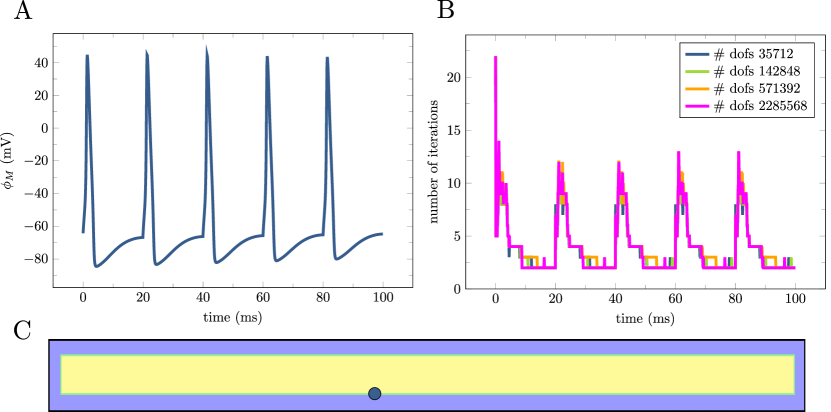
Figure 2: Robustness of the preconditioner with respect to mesh size for model B (idealized 2D axon). The figure displays the temporal evolution of the membrane potential at point $(25,1)$ $\mu$m (A), the total number of iterations over time during refinement in space for the full KNP-EMI system (B), and an illustration of the 2D domain with ICS in yellow and ECS in purple (C).

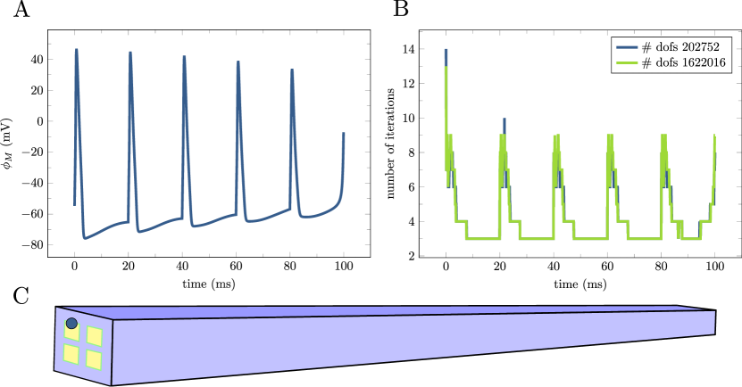
Figure 3: Robustness of the preconditioner with respect to mesh size for model C (idealized 3D axons). The figure displays the temporal evolution of the membrane potential at point $(25,0.3,0.4)$ $\mu$m (A), the total number of iterations over time during refinement in space for the full KNP-EMI system (B), and an illustration of the 3D domain with ICS in yellow and ECS in purple (C).

Problem	Size	Solver	Memory	T${}_{\rm PDE}^{\rm A}$	T${}_{\rm PDE}^{\rm S}$	TPDE
knp-emi	248832	LU	1260	0.52	3.69	4.21
		CG/GMRes (AMG)	614	0.58	1.29	1.67
emi	62208	LU	1260	0.19	1.03	1.22
		CG (AMG)	614	0.25	0.21	0.26
knp	186624	LU	1260	0.33	2.66	2.99
		GMRes (AMG)	614	0.33	1.08	1.41

Table 5: Comparison of average CPU timings and memory usage for the preconditioned iterative solver (CG/GMRes + AMG) and a direct solver (LU) for model C (idealized 3D axons). Size: linear system size (number of degrees of freedom), Memory: maximal memory (MiB) usage of simulation relative to baseline. ${\rm T}_{\rm PDE}^{\rm A}$:  Average CPU time (s) for finite element assembly for one global time step, ${\rm T}_{\rm PDE}^{\rm S}$: Average CPU time (s) for linear system solution for one global time step, ${\rm T}_{\rm PDE}$: Average total CPU time (s) for PDE simulation for one global time step.

6.4 Parallel scalability

The splitting schemes presented in Section 4 result in a solution algorithm where three sub-systems must be solved, namely the EMI and the KNP sub-problems and the ODE system. We next assess how the CPU times for solving the three sub-problems scale with the number of processors. Specifically, we perform two scaling studies: (i) a strong scaling study were we consider an increasing number of cores using the setup in model C, and (ii) a weak scaling study where we increase the mesh resolution and the number of cores simultaneously, such that the number of degrees of freedom per core stays constant, using the setup in model B.

The CPU time required to assemble and solve both the EMI and the KNP sub-problems decreases linearly with the number of cores, which is close to the expected (and ideal) linear scaling (Figure 4A). Similarly, the CPU time for the ODEs scales linearly until we reach $\sim 50$ cores, where the CPU time flattens out.

In the weak scaling study, we observe a sub-linear scaling of the CPU time per core for both assembling and solving the EMI and the KNP sub-problems, whereas the CPU time per core for solving the ODE stays constant (Figure 4B). As the number of degrees of freedom, and consequently the size of the matrix, per core is constant, the ideal scaling is constant.

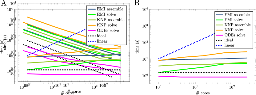
Figure 4: Parallel scalability of assembly and solve times for the EMI and the KNP sub-problems, and for solving the ODEs. Strong scaling data for model C (idealized 3D geometry), with ideal scaling reported (A, log-log plot). Weak scaling data for model B (idealized 2D geometry), with both ideal and linear scaling reported (B, log-log plot). The timings represent total runtime and assembly over 10 timesteps.

6.5 Ion transport is locally dominated by drift

To assess the advective and diffusive contributions to ion transport in physiologically relevant setting for excitable tissue, we run simulations using model C and calculate the (spatially and temporally varying) ratio given by (45) for three different time-points: (i) at 3 ms when an action potential peaks, (ii) at 50 ms when the neuron is at rest, and (iii) at 70 ms where the neuron is severely depolarized. Recall that the ratio is negative where advection dominates (cf. Section 5.6). We observe that advection dominates locally in space during action potential firing, for both ICS and ECS $\rm Na^{+}$, $\rm K^{+}$ (Figure 5), and $\rm Cl^{-}$ (results not shown). Specifically, the ECS ratio during an action potential (at 3 ms) peaks at $-6500$ and $-4000$ for $\rm Na^{+}$ and $\rm K^{+}$, respectively. The ratio is close to zero outside the spatial and temporal zone of the peak, indicating that the advection dominance is local and related to the positioning of the action potential.

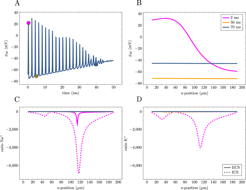
Figure 5: Diffusive and advective contributions of ion transport in model C (idealized 3D axons). The two upper panels display the temporal (A) and spatial (B) evolution of the membrane potential recorded at respectively the point $x=(100,0.5,0.5)$ $\mu$m and at 20 ms (pink), 50 ms (orange) and 70 ms (blue). The lower panels display the ratio between diffusion and advection for transport of $\rm Na^{+}$ (C) and $\rm K^{+}$ (D) where solid lines and dashed lines are respectively ECS and ICS traces of the ratio along the $x$-axis. Recall that the ratio is positive where diffusion dominates, and negative where drift dominates.

6.6 Physiologically realistic 3D simulation

We here consider a geometry based on a digital reconstruction of a pyramidal neuron (model D) to assess how our proposed solver behaves on a realistic geometry. Action potentials are induced every $20$ ms near the tip of the dendrites. The resulting membrane depolarization spreads in space with a conduction velocity of $0.539$ m/s along the axon (Figure 6A,D). The neuronal activity effects the ECS potential locally (Figure 6E) and causes an increase in the ECS $\rm{K}^{+}$ concentration: after $20$ ms the concentration peaks at $4.03$ mM, notably increasing most near the axon and soma (Figure 6F).

Similarly to the models with idealized geometries (models B and C), we observe that the number of iterations before convergence in model D varies with the physical dynamics in the system: the number of iterations peaks at $20$ during the peak of the action potential (at $2$ ms) and decreases to $6$ when the neuron is at rest (Figure 6B).

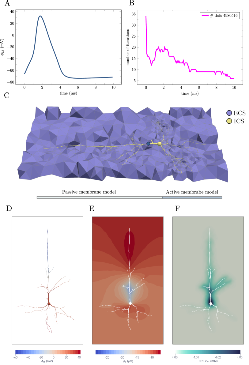
Figure 6: Simulation results with morphologically realistic 3D geometry (model D). The figure displays the temporal evolution of the membrane potential at point $(25,0.3,0.4)$ $\mu$m (A), the total number of iterations for the full KNP-EMI system over simulation time (B), an illustration of the problem domain and mesh (C), snapshots of the membrane potential (D) and the extracellular potential (E) at $t=1.7$ ms, and finally a snapshot of the ECS $K^{+}$ concentration at $t=20$ ms (F).

6.7 Properties of the DG scheme in realistic brain tissue geometries

Brain tissue consist of tightly packed cells separated by thin sheets of ECS. Realistic geometries for numerical simulations of dynamics in collections of brain cells will as such typically be interface dominated (Figure 7A). In $H^{1}$-conforming formulations of the KNP-EMI equations (e.g. the mortar formulation [18] and the multiplier-free formulation [8]), the degrees of freedom at the membrane interfaces will be doubled as they count both in the intra- and extracellular systems, see also Figure 1. Using linear polynomials, we next assess the cost (in terms of system size) of applying DG, which typically leads to a greater number of degrees of freedom (dofs) than conforming formulations, for these interface dominated geometries. We find that the DG discretization results in systems that are $\sim 8$ times larger than that of the conforming formulations (Figure 7B). The same factor is $\sim 14$ for the idealized $3$D mesh in model D (Figure 7B). The cost (in terms of system size) of DG is thus reduced when considering interface dominated geometries.

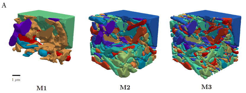
B

mesh	# cells	# dofs mortar	# dofs !LM	# dofs DG	rmortar	r!LM
M1	165211	249076	223512	1982532	7.96	8.87
M2	508644	768698	685896	6103728	7.95	8.90
M3	622294	876556	835472	7467528	8.52	8.94
Model C	124416	108621	105668	1492992	13.7	14.1

Figure 7: Comparison of system size for the mortar [18], multiplier-free [8] and the DG schemes in the case of interface dominated geometries. First order elements are used. Illustrations of interface dominated geometries with 5 (M1), 50 (M2), and 200 (M3) brain cells (ICS) surrounded by ECS (A). Comparison of the number of mesh cells ($\#$ cells), the number of degrees of freedom for the mortar scheme ($\#$ dofs mortar), the conforming multiplier-free scheme ($\#$ dofs !LM) and the DG scheme ($\#$ dofs DG) as well as the ratio between the system sizes of mortar and DG (r_mortar) and of multiplier-free and DG (r_!LM) for the three interface dominated meshes and the idealized 3D mesh from Model C (B).

7 Conclusions and outlook

We have presented a novel solution strategy for solving the KNP-EMI equations which enables their large-scale simulations. The key components of the strategy are: (i) a splitting scheme to decouple the NP equations governing ion transport and the equation arising from the electro-neutrality assumption, (ii) a single dimensional/multiplier-free formulation of the decoupled systems and their discontinuous Galerkin discretization, and (iii) their robust and scalable solvers. Numerical investigations show that the proposed discretization scheme is accurate and converges at expected rates in relevant norms, and that the solution strategy is robust with respect to discretization parameters – both for idealized and realistic two and three dimensional geometries. Strong and weak scaling experiments further show that the parallel scalability of the solver is close to optimal.

Previously the KNP-EMI problem has been solved monolithically [31, 18, 9]. We here introduced a splitting scheme resulting in two smaller and importantly more standard sub-problems, namely an EMI problem and a series of advection diffusion problems, that are discretized and solved using established techniques. For relevant time steps in the neuroscience scenarios considered here, we observe that the splitting scheme is stable. As applications of KNP-EMI models extend beyond neuroscience, to e.g. modelling of Li-ion batteries [47, 25], where other temporal scales may apply, obtaining a better understanding of the accuracy and stability of the splitting scheme via rigorous analysis would be of interest.

The DG scheme is flexible in the sense that its implementation only requires standard functionally in the finite element software used. Further, the DG scheme ensures local mass conservation in each of the sub-problems. However, the DG scheme results in systems with more degrees of freedom than conforming discretizations. A thorough comparison, addressing e.g. accuracy, computational cost and conservation properties, of the previously presented schemes [18, 9, 23, 14] would be valuable.

Concerning practical applications, highly detailed reconstructions of brain tissue and cellular geometries have become available with recent advancements in image technology (see e.g. [13, 33]). New and scalable solution algorithms for geometrically explicit models, such as the KNP-EMI model, allow for new high-fidelity in-silico models taking full advantage of data-sets describing the tissue morphology. Such models could be used to e.g. study how the morphology of cellular processes or the spatial distribution of ionic membrane channels affect transport and buffering in brain tissue, potentially giving new insight into brain signalling and homeostasis in physiology and pathology.

Conflict of interest

The authors declare that they have no conflict of interest.

References

- [1] R. Adams and J. Fournier, Sobolev Spaces, ISSN, Elsevier Science, 2003.
- [2] A. Agudelo-Toro, Numerical simulations on the biophysical foundations of the neuronal extracellular space, PhD thesis, Niedersächsische Staats-und Universitätsbibliothek Göttingen, 2012.
- [3] M. Alnæs, J. Blechta, J. Hake, A. Johansson, B. Kehlet, A. Logg, C. Richardson, J. Ring, M. E. Rognes, and G. N. Wells, The FEniCS project version 1.5, Archive of numerical software, 3 (2015).
- [4] P. Amestoy, I. S. Duff, J. Koster, and J.-Y. L’Excellent, A fully asynchronous multifrontal solver using distributed dynamic scheduling, SIAM Journal on Matrix Analysis and Applications, 23 (2001), pp. 15–41.
- [5] P. F. Antonietti and L. Melas, Algebraic multigrid schemes for high-order nodal discontinuous Galerkin methods, SIAM Journal on Scientific Computing, 42 (2020), pp. A1147–A1173.
- [6] D. N. Arnold, F. Brezzi, B. Cockburn, and L. D. Marini, Unified analysis of discontinuous Galerkin methods for elliptic problems, SIAM journal on numerical analysis, 39 (2002), pp. 1749–1779.
- [7] S. Balay et al., PETSc/TAO users manual, Tech. Report ANL-21/39 - Revision 3.20, Argonne National Laboratory, 2023.
- [8] P. Benedusi, A. J. Ellingsrud, H. Herlyng, and M. E. Rognes, Scalable approximation and solvers for ionic electrodiffusion in cellular geometries, 2024, https://arxiv.org/abs/2403.04491.
- [9] P. Benedusi, P. Ferrari, M. Rognes, and S. Serra-Capizzano, Modeling excitable cells with the EMI equations: spectral analysis and iterative solution strategy, Journal of Scientific Computing, 98 (2024), p. 58.
- [10] N. Berre, M. E. Rognes, and A. Massing, Cut finite element discretizations of cell-by-cell EMI electrophysiology models, arXiv preprint arXiv:2306.03001, (2023).
- [11] A. Budisa, X. Hu, M. Kuchta, K.-A. Mardal, and L. T. Zikatanov, Algebraic multigrid methods for metric-perturbed coupled problems, arXiv preprint arXiv:2305.06073, (2023).
- [12] K. C. Chen and C. Nicholson, Spatial buffering of potassium ions in brain extracellular space, Biophysical journal, 78 (2000), pp. 2776–2797.
- [13] M. Consortium, J. A. Bae, M. Baptiste, C. A. Bishop, A. L. Bodor, D. Brittain, J. Buchanan, D. J. Bumbarger, M. A. Castro, B. Celii, et al., Functional connectomics spanning multiple areas of mouse visual cortex, BioRxiv, (2021), pp. 2021–07.
- [14] G. R. de Souza, R. Krause, and S. Pezzuto, Boundary integral formulation of the cell-by-cell model of cardiac electrophysiology, Engineering Analysis with Boundary Elements, 158 (2024), pp. 239–251.
- [15] E. J. Dickinson, J. G. Limon-Petersen, and R. G. Compton, The electroneutrality approximation in electrochemistry, Journal of Solid State Electrochemistry, 15 (2011), pp. 1335–1345.
- [16] I. Dietzel, U. Heinemann, and H. Lux, Relations between slow extracellular potential changes, glial potassium buffering, and electrolyte and cellular volume changes during neuronal hyperactivity in cat, Glia, 2 (1989), pp. 25–44, http://onlinelibrary.wiley.com/doi/10.1002/glia.440020104/full.
- [17] A. J. Ellingsrud, Supplementary material (code) A splitting, discontinuous Galerkin solver for the cell-by-cell electroneutral Nernst-Planck framework, Apr. 2024, https://doi.org/10.5281/zenodo.10953504, https://doi.org/10.5281/zenodo.10953504.
- [18] A. J. Ellingsrud, A. Solbrå, G. T. Einevoll, G. Halnes, and M. E. Rognes, Finite element simulation of ionic electrodiffusion in cellular geometries, Frontiers in Neuroinformatics, 14 (2020), p. 11.
- [19] R. D. Falgout and U. M. Yang, hypre: A library of high performance preconditioners, in Computational Science — ICCS 2002, P. M. A. Sloot, A. G. Hoekstra, C. J. K. Tan, and J. J. Dongarra, eds., Springer Berlin Heidelberg, 2002.
- [20] A. Hindmarsh and L. Petzold, LSODA, ordinary differential equation solver for stiff or non-stiff system, (2005).
- [21] A. C. Hindmarsh, ODEPACK: Ordinary differential equation solver library. Astrophysics Source Code Library, record ascl:1905.021, May 2019.
- [22] Y. Hu, T. Schneider, B. Wang, D. Zorin, et al., Fast tetrahedral meshing in the wild, ACM Transactions on Graphics (TOG), 39 (2020), pp. 117–1.
- [23] N. M. M. Huynh, F. Chegini, L. F. Pavarino, M. Weiser, and S. Scacchi, Convergence analysis of BDDC preconditioners for composite DG discretizations of the cardiac cell-by-cell model, SIAM Journal on Scientific Computing, 45 (2023), pp. A2836–A2857.
- [24] E. Kaasschieter, Preconditioned conjugate gradients for solving singular systems, Journal of Computational and Applied Mathematics, 24 (1988), pp. 265–275.
- [25] M. Kespe, S. Cernak, M. Gleiß, S. Hammerich, and H. Nirschl, Three-dimensional simulation of transport processes within blended electrodes on the particle scale, International Journal of Energy Research, 43 (2019), pp. 6762–6778.
- [26] C. Koch, Biophysics of computation: information processing in single neurons., Oxford University Press: New York, 1st ed., 1999.
- [27] W. Krassowska and J. C. Neu, Response of a single cell to an external electric field, Biophysical journal, 66 (1994), pp. 1768–1776.
- [28] M. Kuchta, K.-A. Mardal, and M. E. Rognes, Solving the EMI equations using finite element methods, Modeling Excitable Tissue: The EMI Framework, (2021), pp. 56–69.
- [29] A. Logg, K.-A. Mardal, and G. Wells, Automated solution of differential equations by the finite element method: The FEniCS book, vol. 84, Springer Science & Business Media, 2012.
- [30] R. Masri, K. Kirk, E. Hauge, and M. Kuchta, Discontinuous Galerkin methods for the EMI equations, (in prep.), (2024).
- [31] Y. Mori and C. Peskin, A numerical method for cellular electrophysiology based on the electrodiffusion equations with internal boundary conditions at membranes, Communications in Applied Mathematics and Computational Science, 4 (2009), pp. 85–134.
- [32] K. Mörschel, M. Breit, and G. Queisser, Generating neuron geometries for detailed three-dimensional simulations using AnaMorph, Neuroinformatics, 15 (2017), p. 247—269.
- [33] A. Motta, M. Berning, K. M. Boergens, B. Staffler, M. Beining, S. Loomba, P. Hennig, H. Wissler, and M. Helmstaedter, Dense connectomic reconstruction in layer 4 of the somatosensory cortex, Science, 366 (2019).
- [34] C. Nicholson, G. Ten Bruggencate, H. Stockle, and R. Steinberg, Calcium and potassium changes in extracellular microenvironment of cat cerebellar cortex, Journal of neurophysiology, 41 (1978), pp. 1026–1039.
- [35] J. Pods, A comparison of computational models for the extracellular potential of neurons, Journal of Integrative Neuroscience, 16 (2017), pp. 19–32.
- [36] W. Rall, Core conductor theory and cable properties of neurons, in Handbook of Physiology, E. Kandel, J. Brookhardt, and Mountcastle V.M., eds., American Physiological Society, Bethesda, 1977, ch. 3, pp. 39–97, http://onlinelibrary.wiley.com/doi/10.1002/cphy.cp010103/full.
- [37] R. Rasmussen, J. O’Donnell, F. Ding, and M. Nedergaard, Interstitial ions: A key regulator of state-dependent neural activity?, Progress in Neurobiology, (2020), p. 101802.
- [38] B. Rivière, Discontinuous Galerkin methods for solving elliptic and parabolic equations: theory and implementation, SIAM, 2008.
- [39] G. Rosilho de Souza, R. Krause, S. Pezzuto, et al., Boundary integral formulation of the cell-by-cell model of cardiac electrophysiology, Engineering Analysis with Boundary Elements, 158 (2024), pp. 239–251.
- [40] T. Roy, J. Andrej, and V. A. Beck, A scalable DG solver for the electroneutral Nernst-Planck equations, Journal of Computational Physics, 475 (2023), p. 111859.
- [41] G. G. Somjen, Mechanisms of spreading depression and hypoxic spreading depression-like depolarization, Physiol Rev, 81 (2001), pp. 1065–1096, http://physrev.physiology.org/content/81/3/1065.full-text.pdf+html.
- [42] D. Sterratt, B. Graham, A. Gillies, G. Einevoll, and D. Willshaw, Principles of computational modelling in neuroscience, Cambridge university press, 2023.
- [43] J. Sundnes, G. T. Lines, X. Cai, B. F. Nielsen, K.-A. Mardal, and A. Tveito, Computing the electrical activity in the heart, vol. 1, Springer Science & Business Media, 2007.
- [44] E. Syková and C. Nicholson, Diffusion in brain extracellular space, Physiol Rev, 88 (2008), pp. 1277–1340, https://doi.org/10.1152/physrev.00027.2007.
- [45] A. Tveito, K. H. Jæger, M. Kuchta, K.-A. Mardal, and M. E. Rognes, A cell-based framework for numerical modeling of electrical conduction in cardiac tissue, Frontiers in Physics, 5 (2017), p. 48.
- [46] A. Tveito, K.-A. Mardal, and M. E. Rognes, Modeling excitable tissue: The EMI framework, Springer Nature, 2021.
- [47] A. H. Wiedemann, G. M. Goldin, S. A. Barnett, H. Zhu, and R. J. Kee, Effects of three-dimensional cathode microstructure on the performance of lithium-ion battery cathodes, Electrochimica Acta, 88 (2013), pp. 580–588.
- [48] B. I. Wohlmuth, A -cycle multigrid approach for mortar finite elements, SIAM journal on numerical analysis, 42 (2005), pp. 2476–2495.
- [49] K. Xylouris, G. Queisser, and G. Wittum, A three-dimensional mathematical model of active signal processing in axons, Computing and visualization in science, 13 (2010), pp. 409–418.
- [50] W. Ying and C. S. Henriquez, Hybrid finite element method for describing the electrical response of biological cells to applied fields, IEEE transactions on biomedical engineering, 54 (2007), pp. 611–620.