Boosting Self-Supervision for Single-View Scene Completion
via Knowledge Distillation

Abstract

Inferring scene geometry from images via Structure from Motion is a long-standing and fundamental problem in computer vision. While classical approaches and, more recently, depth map predictions only focus on the visible parts of a scene, the task of scene completion aims to reason about geometry even in occluded regions. With the popularity of neural radiance fields, implicit representations also became popular for scene completion by predicting so-called density fields. Unlike explicit approaches e.g. voxel-based methods, density fields also allow for accurate depth prediction and novel-view synthesis via image-based rendering. In this work, we propose to fuse the scene reconstruction from multiple images and distill this knowledge into a more accurate single-view scene reconstruction. To this end, we propose Multi-View Behind the Scenes (MVBTS) to fuse density fields from multiple posed images, trained fully self-supervised only from image data. Using knowledge distillation, we use MVBTS to train a single-view scene completion network via direct supervision called KDBTS. It achieves state-of-the-art performance on occupancy prediction, especially in occluded regions.

Figure 1: Knowledge Distillation from Multi-View to Single-View. We propose to boost single-view scene completion by exploiting additional information from multiple images. a) we first train a novel multi-view scene reconstruction algorithm that is able to fuse density fields from multiple images in a fully self-supervised manner. b) we then employ knowledge distillation to directly supervise a state-of-the-art single-view reconstruction model in 3D to boost its performance. https://keonhee-han.github.io/publications/kdbts/

1 Introduction

Obtaining accurate 3D geometry of a scene is crucial to achieving a holistic understanding of our surroundings. This knowledge enables a plethora of tasks both in robotics and autonomous driving. Reconstructing the scene’s geometry from raw images, also called Structure-from-Motion [43], is a long-standing task in computer vision. Classical methods of scene reconstruction rely on multiple images and triangulation of matched keypoints, such as Harris Corner Detection, SIFT, and ORB [17, 35, 42], to infer the geometry of a scene. More recently, the breakthrough of deep learning gave rise to monocular depth estimation (MDE) methods [12, 13], that allowed to predict a dense per pixel depth from only a single image. These are either trained with ground truth supervision or in a self-supervised manner from video data [64, 58, 13, 36, 16, 45, 57, 14, 50]. Despite the impressive results of MDE for geometry estimation, the depth map representations are limited in their expressiveness. Projecting them into other frames will lead to holes or possibly wrong estimates due to occlusions in the scene. Furthermore, they cannot make any statements about the scene beyond the visible surfaces.

Scene reconstruction broadens the task of scene representation from depth maps to reasoning about the whole geometry of a scene, including occluded regions [46] by doing shape completion. [46] introduced the task of semantic scene completion, which extends scene reconstruction to include semantic predictions. The 3D nature of both tasks results in many methods relying on voxel representations for their predictions that either use images [4, 31] or LiDAR/depth maps [41, 46] as input.

Neural implicit representations in the form of neural fields offer an alternative scene representation. Popularized by NeRFs, which models a scene’s geometry and view-dependent colors in the weights of a neural network, they allow for photorealistic novel view synthesis. However, the original NeRF work [38] cannot generalize to different scenes and often suffers from inaccurate geometry [48]. These limitations were addressed by many follow-up works to NeRF [56, 39, 48]. Similarly, density fields [52] solely model the scene’s geometry, addressing the geometric inconsistencies of NeRFs. The work Behind the Scenes (BTS) [52] uses density fields predicted from a single image for scene completion, while IBRnet and NeuRay leverage density predictions from multiple images together with images-based rendering for novel-view synthesis. MVBTS presents an extension of BTS from a single image to multiple images for more accurate scene reconstructions. In the absence of accurate 3D ground truth geometry, we leverage these scene reconstructions to directly supervise single-view density prediction models. We retrain the original BTS architecture in this pseudo-supervised setting as KDBTS to boost its performance. We release the code to further facilitate research.

Our contributions within this work are threefold:

• We extend the density field prediction of BTS to a multi-view setting trained in a fully self-supervised manner.

• We propose knowledge distillation training to directly supervise single-view density fields on fused multi-view predictions.

• Our method achieves state-of-the-art performance for both multi- and single-view occupancy prediction on the KITTI-360 benchmark.

2 Related Work

Neural Scene Representations nerf [38] has popularized the method of representing a scene with neural implicit functions. nerf allows to query color and occupancy of a scene in continuous space by storing the scene within the weights of a neural network. This allows NeRF to do photorealistic novel view synthesis (NVS) of a scene. A downside of the original NeRF is the need to retrain the network weights for each scene. This was addressed by works such as PixelNeRF [56] and MINE [29] that construct neural radiance fields on the fly conditioned on sparse input views. [44] maps 2D image observations of a scene to a persistent 3D scene representation, disentangling movable and immovable components of the scene. Neo360 [22] uses a tri-planar representation together with foreground and background MLPs to allow for representing unbounded scenes.

However, most NeRF methods focus on tasks such as novel view synthesis, often leading to inaccurately reconstructed scene geometry. Works such as [48] address this by modeling effects such as reflections on surfaces.

Image Based Rendering Imaged-based rendering synthesizes images for novel views based on the color of surrounding reference images. Early methods focused on blending reference pixels based on geometry proxies [1, 8, 21]. Other works on light fields reconstruct 4D plenoptic functions from input views [15, 7]. More recent approaches are based on NeRF architectures. IBRnet [49] uses input images to construct a radiance field and density field on the fly. The density is predicted from pooled feature vectors in a ray transformer, sharing information between 3D points. The color is reconstructed as a weighted sum of the colors of surrounding views. GeoNeRF [23] uses cost volumes together with an attention-based aggregation for density prediction while replacing the ray transformer with an autoencoder. NeuRay [34] addresses the problem of inconsistent image features due to occlusions. Based on either cost volumes or depth maps, it predicts the visibility of 3D points in different views, leading to better renderings.

Scene Completion Scene completion, sometimes also called scene reconstruction, refers to the task of estimating the 3D geometry of a scene from images. Depending on the task, scene completion can range from depth prediction [12, 13, 47, 37, 51] to reconstructing even occluded parts of a scene [52, 4]. Depth prediction can either come from monocular images [13, 62] or stereo images [59, 24]. Especially MDE has been successfully used in monocular visual odometry applications [55, 25].

The information from depth prediction is restricted to the visible surfaces of a scene, leaving out important information about the shapes of objects. Given a depth map [10, 53, 46] complete shape geometry in an environment using voxel-grid representations. Voxlets [10] use random forests to predict signed distance values in the grid, whereas [53] models a probabilistic distribution on voxels. Generalizable NeRF methods such as PixelNeRF [56] and MINE [29] can also be used to complete the scene geometry. Recently, Behind the Scenes (BTS) [52] introduced a density field representation based on NeRF to model the scene geometry implicitly together with imaged-based rendering to explicitly learn to “look behind” objects.

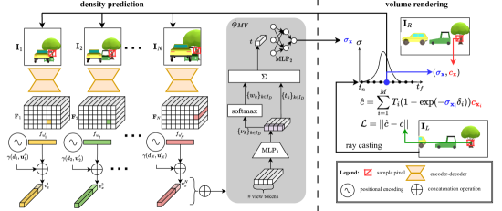
Figure 2: Overview. Given multiple input images $\textbf{I}_{k}$ ($k\in I_{D}$) an encoder-decoder backbone predicts per image a pixel-aligned feature map $\textbf{F}_{k}$ (top left). The feature $f_{\textbf{u}}$ of pixel u encodes the occupancy and confidence distribution of a ray cast through pixel u. Given a 3D point x and its projections $\textbf{u}^{\prime}_{k}$ into the different camera images, we extract the corresponding feature vectors and positional embeddings $\gamma(d,\textbf{u})$. A multi-view network $\phi_{\text{MV}}$ decodes all feature vectors into a density prediction $\sigma_{\textbf{x}}$ (middle). Together with color samples from another image ($\textbf{I}_{R}$), this can be used to render novel views in an image-based rendering pipeline. $\textbf{I}_{R}$ is not required to be close to the input images, as our method can predict density in occluded regions. See Fig. 3 for more details about the importance of covering the whole scene. We train our networks by using a photometric consistency loss of an image $\textbf{I}_{L}$ close to $\textbf{I}_{R}$ (right).

ssc, first introduced in [46], extends this task even further to the semantic setting. For occupied regions, semantic labels are predicted. In the beginning, semantic scene completion (SSC) methods either focused on indoor scenarios with image data [60, 61, 33, 27, 26, 28, 5, 2] or outdoor scenarios with LiDAR data [41, 6, 54, 30, 40]. MonoScene [4] was the first method to tackle outdoor scenarios from image data by using line-of-sight projection of deep image features. VoxFormer [31] utilizes a transformer architecture with deformable attention layers. Both rely on voxels for their scene representation. S4C [18] uses an implicit scene representation and a self-supervised training approach to remove the need for annotated 3D data.

In this work, we build upon the ideas of scene completion methods from single images, BTS [52]. Specifically, to exploit all the available image data at inference time for more accurate occupancy predictions. We then leverage our accurate predictions to further improve single-image scene completion. This is in contrast to the works of [49, 34, 23] that focus on NVS and rely on close-by views to provide both color and density information.

3 Method

In the following, we briefly recap the Behind the Scenes (BTS) model as we extend its architecture and use it in our knowledge distillation scheme. We also cover training setup to predict the scene’s geometry, even in occluded areas. We then introduce the extension of the BTS architecture to a multi-view setting and propose a knowledge distillation scheme for improved single-view predictions.

Notation We denote images by $\textbf{I}_{k}\in[0,1]^{3\times H\times W}=(\mathbb{R}^{3})^{\Omega}$ which are defined on a lattice $\Omega=\{1,\ldots,H\}\times\{1,\ldots,W\}$. The corresponding camera poses and projection matrices of the images are given as $T_{i}\in\mathbb{R}^{4\times 4}$ and $K_{i}\in\mathbb{R}^{3\times 4}$, respectively. The density of a point $\textbf{x}\in\mathbb{R}^{3}$ in world coordinates is given by $\sigma_{\textbf{x}}$. Its projection into an image $k$ is given by $\pi_{k}(\textbf{x})=K_{k}T_{k}\textbf{x}$ in homogeneous coordinates. From our set of all image indices $I=\{1,\ldots,N\}$, we create the following subsets $I_{D}$, $I_{L}$, and $I_{R}$ for density, loss, and render. For these subsets, the following holds:

$$I_{D}\subset I$$ (1)

$$I_{L}\cup I_{R}=I$$ (2)

$$I_{L}\cap I_{R}=\emptyset$$ (3)

We give examples together with a more detailed explanation for these splits in the supplementary material.

3.1 Prerequisites: Density Field from a Single View

BTS models a scene by predicting a volumetric density for a 3D point x conditioned on an input image $\textbf{I}_{\text{I}}$ [52]. This is done by predicting a pixel-aligned feature map $\textbf{F}_{\text{I}}\in(\mathbb{R}^{C})^{\Omega}$ with an encoder-decoder architecture from the image. The point x is projected into the input image $\textbf{u}^{\prime}_{\text{I}}=\pi_{\text{I}}(\textbf{x})$ to obtain the corresponding feature vector $f_{\textbf{u}^{\prime}}=\textbf{F}(\textbf{u}^{\prime})$ from the feature map. A small multi-layer perceptron (MLP) $\phi_{SV}$ decodes the density from the feature vector as well a positional encoding $\gamma(d_{\text{I}},\textbf{u}^{\prime}_{\text{I}})$ of the depth $d_{\text{I}}$ and pixel position $\textbf{u}^{\prime}_{\text{I}}$ as

$$\sigma_{\textbf{x}}=\phi_{SV}(f_{\textbf{u}^{\prime}_{\text{I}}},\gamma(d_{\text{I}},\textbf{u}^{\prime}_{\text{I}}))$$ (4)

The intuition behind this density prediction is that the feature vector of a pixel learns to describe the density distribution along the corresponding ray [52]. Together with the positional encodings, the MLP ($\phi_{SV}$) decodes this distribution into a density prediction.

3.2 MVBTS: Density Field from Multiple Views

We extend the single-view density prediction by replacing the $\phi_{SV}$ with a confidence-based multi-view architecture

$$\sigma_{\textbf{x}}=\phi_{MV}(\{f_{\textbf{u}^{\prime}_{k}},\gamma(d_{k},\textbf{u}^{\prime}_{k})\}_{k\in I_{D}})\,,$$ (5)

that is able to aggregate the information from the $|I_{D}|$ images. In the following, we will break down how to predict a density value for a point x from multiple input images.

For each of the input images $\{\textbf{I}_{k}\}_{k\in I_{D}}$, we predict a pixel-aligned feature map $\textbf{F}_{k}$ with a shared encoder-decoder architecture. The point x is then projected into each of the input images $\textbf{u}^{\prime}_{k}=\pi_{k}(\textbf{x})$, giving us $|I_{D}|$ feature vectors $f_{\textbf{u}^{\prime}_{k}}=\textbf{F}_{k}(\textbf{u}^{\prime}_{k})$. We keep track of valid projections into the frustum of a camera with a binary masking vector $\textbf{m}\in\{0,1\}^{|I_{D}|}$. The feature vectors are concatenated with the respective positional encodings $\gamma(d_{k},\textbf{u}^{\prime}_{k})$ and fed through a small MLP

$$(\nu_{k},t_{k})=\text{MLP}_{1}(f_{\textbf{u}^{\prime}_{k}},\gamma(d_{k},\textbf{u}^{\prime}_{k}))$$ (6)

to produce both a confidence $\nu_{k}$ and a view-dependent features $t_{k}$. A softmax layer then converts the confidence values into weights

$$\{w_{k}\}_{k\in I_{D}}=\text{softmax}(\{\nu_{k}\}_{k\in I_{D}},\textbf{m})\,,$$ (7)

that are then used in a weighted summation

$$t=\sum_{k\in I_{D}}w_{k}t_{k}$$ (8)

to produce a view-aggregated feature $t$. This feature is then decoded by a second MLP to produce the density estimate

$$\sigma_{\textbf{x}}=\text{MLP}_{2}(t)\,.$$ (9)

For more details, see the left-hand side of Fig. 2.

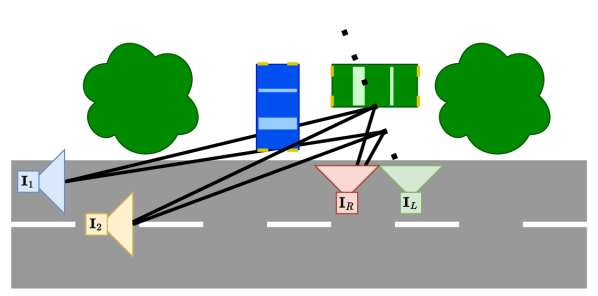
Figure 3: Training Setup. Given an input view ($\textbf{I}_{\text{1}}$, blue) we want to reconstruct the scene, including partially occluded objects such as the green car. To learn to reconstruct both the free space behind the blue car and the surface of the green car, we try to render a pixel of the green view ($\textbf{I}_{\text{L}}$) by casting a ray and sampling points on it (dotted line). We project the points into the blue view to estimate the density and into the red view ($\textbf{I}_{\text{R}}$) to sample colors. The pixel of $\textbf{I}_{\text{L}}$ is only reconstructed correctly if $\textbf{I}_{\text{1}}$ estimates the correct density of the scene, although the green car and the free space next to it is occluded. In our multi-view method, we propose to use more views, e.g. the yellow view $\textbf{I}_{\text{2}}$ to aggregate more information about the scene to better density predictions. In this example, the yellow view has a slightly better visibility on the green car.

3.3 Training via Volumetric Rendering

For convenience, this section recaps the training scheme from BTS [52], which we follow closely. As with BTS, this work aims to predict accurate 3D geometry with a continuous scene representation trained only on posed images in a self-supervised manner. We use our geometry prediction and image-based rendering techniques in a differentiable volumetric rendering pipeline to reconstruct images, allowing us to leverage a photometric reconstruction loss to train our networks. See the right-hand side of Fig. 2 for an overview of the volumetric rendering.

Color Sampling. Unlike most NeRF models, we do not predict color that is used to render novel views directly. Instead, we rely on other images to provide us with color samples. Given the point x and a frame $k\in I_{R}$, we obtain a color sample $c_{\textbf{x},k}$ by projecting x into frame $k$ and interpolating the color value of the image $c_{\textbf{x},k}=\textbf{I}_{k}(\textbf{u}^{\prime}_{k})$.

Volumetric rendering. To render a pixel for NVS from an image $\textbf{I}_{L}$, we cast a ray from the camera through the pixel. We sample $M$ discrete points along the ray at positions $\textbf{x}_{i}$. This discrete sampling lets us approximate the continuous volume rendering equation [38]. For each point, we extract its density $\sigma_{\textbf{x}_{i}}$ from our multi-view density field and colors $c_{\textbf{x}_{i},k}$ from different images $k\in I_{R}$. We render the color of a pixel by aggregating the sampled colors over the density distribution on the ray

$$\hat{c}_{k}=\sum_{i=1}^{M}T_{i}\alpha_{i}c_{\textbf{x}_{i},k}\,,$$ (10)

with $\alpha_{i}$, the probability of the ray ending between $\textbf{x}_{i}$ and $\textbf{x}_{i+1}$, $\delta_{i}$, the distance between $\textbf{x}_{i}$ and $\textbf{x}_{i+1}$, and $T_{i}$, the accumulated transmittance, given by

$$\alpha_{i}=1-\exp(-\sigma_{\textbf{x}_{i}}\delta_{i})\quad\quad T_{i}=\prod_{j=1}^{i-1}(1-\alpha_{j})\,.$$ (11)

Based on the density and $d_{i}$, the distance between $\textbf{x}_{i}$ and the ray origin, we can also calculate the expected ray termination depth

$$\hat{d}=\sum_{i=1}^{m}T_{i}\alpha_{i}d_{i}\,.$$ (12)

We want to note that this volumetric rendering reconstructs multiple color suggestions $\hat{c}_{k}$ for a single pixel based on the different frames $k$, where the color samples come from.

A key insight of BTS was the setup of the cameras during training. Separating rendering, color sampling, and density prediction to different views allows one to learn the density even in occluded regions of the image. We follow this training setup, adapted to account for multiple input views; see Fig. 3 for more details on this.

Loss functions. We do not reconstruct individual pixels for training the networks, but rather patches of pixels $P_{i}$, randomly sampled from the loss images $\textbf{I}_{L}$. Our reconstruction loss is a photometric-consistency loss, combining an L1 and an SSIM loss, following the strategy of [52, 13] of only selecting the per-pixel minimum over the reconstructions $\hat{P}_{i,k}$ when aggregating the costs.

$$\mathcal{L}_{\text{ph}}=\min_{k\in I_{R}}\left(\lambda_{\text{L1}}\text{L1}(P_{i},\hat{P}_{i,k})+\lambda_{\text{SSIM}}\text{SSIM}(P_{i},\hat{P}_{i,k})\right)$$ (13)

Additionally, we also employ an edge-aware smoothness loss term on $d^{\star}$ an inverse parameterized, mean-normalized version of $\hat{d}$,

$$\mathcal{L}_{\text{eas}}=\left|\delta_{x}d^{\star}_{i}\right|e^{-\left|\delta_{x}P_{i}\right|}+\left|\delta_{y}d^{\star}_{i}\right|e^{-\left|\delta_{y}P_{i}\right|}$$ (14)

to regularize the expected ray termination depth, giving us the final loss

$$\mathcal{L}=\mathcal{L}_{\text{ph}}+\lambda_{\text{eas}}\mathcal{L}_{\text{eas}}\,.$$ (15)

We give additional details for the training on the different datasets in Sec. 4.

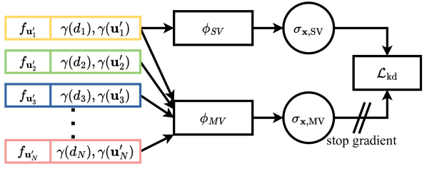
Figure 4: Knowledge Distillation. To improve the single-view (SV) density field reconstruction, we propose leveraging knowledge distillation from the multi-view (MV) predictions. Both $\phi_{\text{SV}}$ and $\phi_{\text{MV}}$ make use of the same encoder-decoder architecture and, therefore, the same feature vectors. The knowledge distillation loss $\mathcal{L}_{\text{kd}}$ pushes the $\phi_{\text{SV}}$ MLP to predict the same density as $\phi_{\text{MV}}$ while relying only upon a single feature vector. The stop gradient operator prevents $\mathcal{L}_{\text{kd}}$ influencing $\phi_{\text{MV}}$.

3.4 KDBTS: Knowledge Distillation for Single-View Reconstruction

Given the scene reconstructions from our multi-view model, we want to distill this knowledge into a single-view prediction model that can reconstruct the scene from fewer input data, e.g. a single image. We use the original BTS model architecture for our KDBTS. The motivation behind our knowledge distillation approach is threefold. First, it reduces the network size, as the decoder is slightly smaller, speeding up the inference time. Second, removing the necessity of pose information at inference time. The advantage of single-view reconstruction is that it neither requires a calibrated stereo camera setup nor relative pose information from visual odometry systems to reconstruct the scene. Third, it leverages the advantages of self-supervised and supervised training. MVBTS can be trained on image data alone, allowing it to scale to vast amounts of data. This allows our method to be employed in the absence of ground truth data and still provide direct supervision by generating a pseudo ground truth. This knowledge distillation scheme is illustrated in Fig. 4.

Given the input images $\textbf{I}_{\text{I}}$ and $\{\textbf{I}_{k}\}_{k\in D}$ for single- and multi-view, respectively, $\sigma_{\textbf{x},\text{SV}}=\phi_{SV}(f_{\textbf{u}^{\prime}_{\text{I}}},\gamma(d_{\text{I}},\textbf{u}^{\prime}_{\text{I}}))$ and $\sigma_{\textbf{x},\text{MV}}=\phi_{MV}(\{f_{\textbf{u}^{\prime}_{k}},\gamma(d_{k},\textbf{u}^{\prime}_{k})\}_{k\in I_{D}})$ should give the same density prediction for a 3D point x. In practice, we choose the input view $\textbf{I}_{\text{I}}$ for the single-view head to be from $\{\textbf{I}_{k}\}_{k\in D}$, but this is not strictly necessary. Knowledge distillation is then performed via a simple L1 loss

$$\mathcal{L}_{\text{kd}}=\|\sigma_{\textbf{x},\text{MV}}-\sigma_{\textbf{x},\text{SV}}\|\,.$$ (16)

To avoid the multi-view head being influenced by the single-view prediction, we apply a stop gradient operator on $\sigma_{\textbf{x},\text{MV}}$ to treat it as a pseudo ground truth.

Dataset	Split.	# Train	# Val	# Test
KITTI	Eigen  [9]	39810	4424	697
KITTI-360	BTS  [52]	98008	11451	446

Table 1: Dataset Split Overview. Number of images in each split of the datasets. Evaluation is performed exclusively on the test splits.

4 Experiments

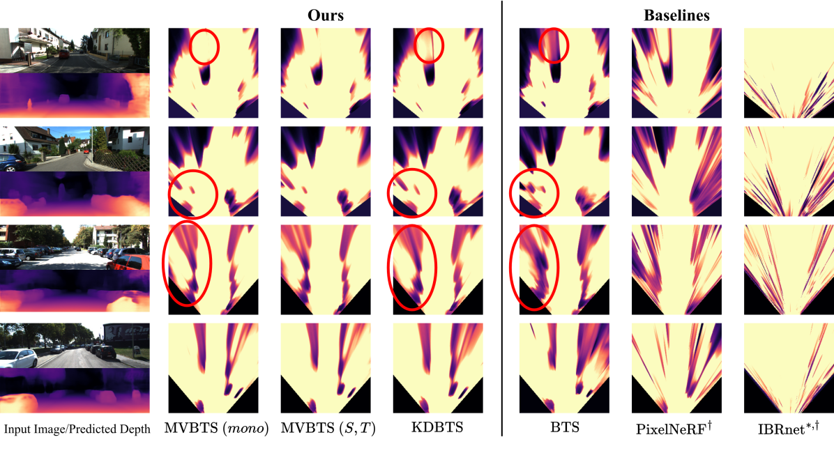
Figure 5: Density Fields. Top-down rendering of the density fields for an area of $x=\left[-9m,9m\right]$, $y=\left[0m,1m\right]$, $z=\left[3m,23m\right]$. Images are taken from KITTI-360 (top half) and KITTI (bottom half) with profiles coming from models trained on KITTI-360. Every model except for MVBTS $(S,T)$ and IBRnet [49] get the same input data. Our MVBTS can predict accurate geometry even in distant regions for both a single image and multiple images. KDBTS learns to recreate the accurate density structure from MVBTS. Both models reduce the amount of shadows produced by BTS [52], especially in distant regions. They also produce cleaner boundaries for close-by objects. Note that KDBTS has a smaller model capacity than MVBTS $(mono)$. $*$: changed sensitivity for visualization purposes, $\dagger$: retrained on KITTI-360.

We demonstrate the advantages of having multiple views to predict density fields in the tasks of depth prediction and occupancy estimation. We evaluate both our multi-view model (MVBTS) as well as our single-view model (KDBTS) boosted by knowledge distillation. We follow the evaluation of [52] and evaluate the depth prediction on the KITTI [11] dataset against the ground truth depth and occupancy estimation on KITTI-360 [32] against occupancy maps from aggregated LiDAR scans over multiple time steps.

4.1 Datasets and Training Details

KITTI [11] and KITTI-360 [32] are both autonomous driving datasets that provide time-stamped stereo images with ground truth poses - although for KITTI we use poses generated by ORB-SLAM 3 [3]. KITTI-360 also provides fisheye cameras looking to the sides. For our training, they are rectified to the same camera intrinsics as the stereo cameras. A randomly applied dropout of $0.5$, helps our model to not overfit on a specific camera setup. During training, we randomly select three stereo input views to be in $I_{D}$.

We train our model on a single 48GB Nvidia RTX A40 GPU with half the batch size of BTS, 8, due to increased memory demand from the multiple views. We sample 32 patches of size $8\times 8$ with 64 points per ray for possible reconstruction. The encoder-decoder follows [52] to be a ResNet50 encoder [20] with 64 output channels. $\text{MLP}_{1}$ and $\text{MLP}_{2}$ are chosen to be two-layer networks with residual connections. $\text{MLP}_{1}$ therefore corresponds to a larger version of the decoder network of BTS, as it needs to decode additional information. For detailed hyperparameters, please refer to the supplementary material.

We train for 150,000 steps on KITTI and for 200,000 steps on KITTI-360, compensating for our smaller batch size. We train on the splits detailed in Tab. 1.

In our experimental setup, both KDBTS and MVBTS share a backbone architecture. To train the KDBTS model, we use a trained MVBTS model and freeze the encoder-decoder backbone as well as $\phi_{MV}$. We found training both in parallel to give a slightly decreased performance. To additionally boost the performance in distant parts of the scene, we randomly sample the timestamp offset of the additional stereo frames between $0.1s$ and $0.8s$. As direct supervision and a shared backbone lead to a strong training signal, we train the knowledge distillation for only 20,000 steps.

4.2 Depth Prediction

Although a byproduct of the density field, depth estimates provide useful information leveraged by downstream tasks, such as segmentation. In Tab. 2, we compare our two methods against self-supervised depth prediction methods and volume reconstruction methods. Fig. 6 shows qualitative results on KITTI. For depth prediction, we keep the same training setup for KITTI so that we report the values for PixelNeRF [56], MonoDepth2 [13], DevNet [63], and BTS [52] from [52]. For more single-view methods, please refer to [52].

Model	Volum.	Abs Rel $\downarrow$	RMSE $\downarrow$	$\alpha<1.25\uparrow$
PixelNeRF [56]	✓	0.130	5.134	0.845
MonoDepth2 [13]	✗	0.106	4.750	0.874
DevNet [63]	(✓)	0.095	4.365	0.895
BTS [52]	✓	0.102	4.407	0.882
KDBTS (Ours)	✓	0.105	4.497	0.873
MVBTS (Ours)	✓	0.105	4.501	0.873

Table 2: Monocular Depth Evaluation. Our method performs very similar to BTS due to the similarity of the architecture. We suspect that the slight differences in the presented metrics arise from some of the model capacity being shifted to better predict the occluded parts of the scene.

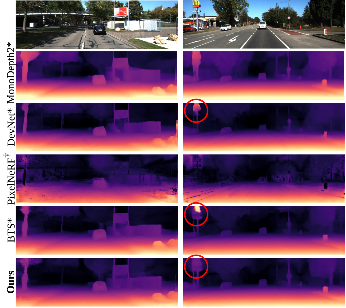
Figure 6: Monocular Depth Prediction. Qualitative comparison with state-of-the-art monocular depth prediction and other volumetric methods. The expected ray termination depth $\hat{d}$ gives a detailed scene reconstruction.

Method	Multi View	$\text{O}_{\text{acc}}\uparrow$	$\text{O}_{\text{prec}}\uparrow$	$\text{O}_{\text{rec}}\uparrow$	$\text{IE}_{\text{acc}}\uparrow$	$\text{IE}_{\text{prec}}$	$\text{IE}_{\text{rec}}\uparrow$
PixelNeRF [56]	✗	93.82%	51.94%	69.43%	61.33%	37.86%	42.21%
BTS [52]	✗	94.47%	58.73%	84.24%	77.04%	54.21%	43.99%
MVBTS (Ours)	✗	94.76%	60.83%	84.51%	78.00%	53.69%	44.04%
KDBTS (Ours)	✗	94.76%	60.68%	84.78%	78.30%	53.62%	44.00%
IBRnet [49]	✓	96.03%	4.14%	4.78%	34.36%	32.97%	96.02%
IBRnet (depth + 4m) [49]	✓	98.12%	43.35%	86.01%	59.67%	25.18%	9.85%
MVBTS (Ours)	✓	94.91%	61.73%	85.78%	79.47%	55.08%	45.23%

Table 3: Occupancy Prediction on KITTI-360. We follow the evaluation setup of BTS [52] and evaluate both the occupancy of the whole scene (O) and only the invisible and empty parts (IE). In both cases, we report accuracy, precision, and recall, as there is a large imbalance between occupied and empty parts of the scene. We evaluate MVBTS and KDBTS in a single-view and MVBTS additionally in a multi-view setting. KDBTS can improve upon the original BTS consistently. Due to IBRnet [49] predicting little density (see Fig. 5), we also evaluate IBRnet in the setting of depth + 4m, giving better occupancy precision and recall.

Inference	dropout	MLPs	attn. layers	encode fisheye	$\text{O}_{\text{acc}}\uparrow$	$\text{O}_{\text{prec}}\uparrow$	$\text{O}_{\text{rec}}\uparrow$	$\text{IE}_{\text{acc}}\uparrow$	$\text{IE}_{\text{prec}}$	$\text{IE}_{\text{rec}}\uparrow$
(S, T)	0.5	middle	✓	✗	-1.67%	-0.96%	-15.09%	-9.64%	-7.67%	13.70%
(S, T)	0.0	middle	✗	✓	-1.47%	-4.88%	-6.04%	-6.45%	-9.54%	-1.33%
(S, T)	0.2	middle	✗	✓	-0.34%	-1.88%	-2.58%	-2.34%	-0.67%	0.41%
(S, T)	0.5	middle	✗	✓	0.02%	-1.01%	-0.31%	-0.42%	0.65%	1.16%
(S, T)	0.8	middle	✗	✓	0.04%	-1.30%	0.62%	-0.06%	0.27%	-0.43%
(S, T)	0.5	small	✗	✗	-0.26%	-2.09%	0.86%	-0.93%	-0.04%	-1.53%
(S, T)	0.5	large	✗	✗	-0.53%	-1.84%	-3.27%	-2.23%	-3.41%	1.66%
(Mono)	0.5	middle	✗	✗	-0.15%	-0.90%	-1.27%	-1.47%	-1.38%	-1.19%
(S)	0.5	middle	✗	✗	-0.07%	-0.61%	-0.50%	-0.85%	-1.06%	-1.19%
(T)	0.5	middle	✗	✗	-0.09%	-0.77%	-0.88%	-0.63%	-1.01%	-0.04%
(S, T)	0.5	middle	✗	✗	94.91%	61.73%	85.78%	79.47%	55.08%	45.23%

Table 4: Ablation Studies. To motivate the choice of our architecture for MVBTS, we detail the results for different settings. We also report the influence of additional images at inference time. Overall, the architecture is robust against the most hyperparameter settings. The ablation study shows that keeping the multi-view aggregation simple. We specifically address the use of attention layers together with a detailed breakdown of the different settings in the supplementary material.

4.3 Occupancy Prediction

The main evaluation of our method is with regard to the occupancy prediction. Next to our method, we evaluate with PixelNeRF [56] and the original BTS [52] two additional single-view reconstruction methods. For multi-view methods, we compare against another image-based rendering method, IBRnet [49] retrained on KITTI-360. Fig. 5 shows top-down renderings of occupancy predictions both on KITTI and KITTI-360 made with models trained on KITTI-360. They show qualitative results for difficult scenarios. For IBRnet, we increased the sensitivity of the visualization as the density values were, on average, significantly lower than for the other methods. Our models reason better in far-away parts of the scene (see first example). Additionally, they produce cleaner occupancy edges in occluded areas of the scene, leading to fewer artifacts. For quantitative evaluation, we follow [52] with carving out free space based on LiDAR scans. We evaluate accuracy, precision, and recall for two settings: 1. Occupancy predictions ($\text{O}_{\text{acc}}$, $\text{O}_{\text{prec}}$, $\text{O}_{\text{rec}}$) and 2. Invisible and empty ($\text{IE}_{\text{acc}}$, $\text{IE}_{\text{prec}}$, $\text{IE}_{\text{rec}}$), giving us six metrics in total. Tab. 3 details the results on KITTI-360. Unlike BTS [52], we also choose to include the precision and recall for the occupancy due to the large imbalance between occupied and empty space. As the distribution is heavily skewed to the empty space, achieving a high accuracy score is easy, as can be seen for IBRnet. On KITTI-360, IBRnet seems to give fog-like predictions with few clear boundaries, as can be seen in Fig. 5, resulting in low precision and recall. We also evaluate IBRnet in the depth + $4m$ setting to address this. This reduces the $\text{IE}_{\text{rec}}$ but gives competitive other metrics. Our models, both MVBTS and KDBTS, are evaluated in the single-view setting in the top half of Tab. 3. Both methods consistently improve the original BTS across most metrics. Despite the lower model capacity, KDBTS performs on par with MVBTS, validating our knowledge distillation approach. In the multi-view setting, where the models have access to four frames - stereo and temporal -, MVBTS performs the most consistently across all metrics. IBRnet has a better $\text{O}_{\text{acc}}$ and, depending on the prediction mode, either a slightly better $\text{O}_{\text{rec}}$ or significantly better $\text{IE}_{\text{rec}}$. We suspect this results from the large imbalance of empty to occupied space. MVBTS either performs on par or significantly better than IBRnet. We present additional evaluation results in the supplementary material.

4.4 Ablation Studies

Tab. 4 gives an overview of the impact different design choices in our architecture and training scheme have on the performance of our model. Our ablation study is split into two parts. In the first part, we are concerned with the architecture of $\phi_{MV}$, whereas ablations on the backbone have already been done in [52]. The second part investigates the influence of the number of available views on the performance of the model. For our ablation study, we use our final model as a baseline and report the differences to this model in the table. We investigate the following: adding attention layers similar to GeoNeRF [23] for enhanced information sharing between views; also including fisheye views in $I_{D}$; the effects of different dropout rates; the size of the MLPs. In general, our method shows robust performance in the ablation settings. Attention layers allow for information sharing between tokens and can implicitly learn to shift focus to certain views. However, within this architecture, they seem to hinder the model’s performance. We detail a possible explanation together with examples in the supplementary material. Including fisheye cameras leads to a mostly on-par performance. This is likely due to most sampled points lying outside of the fisheye cameras’ frustums. Less dropout leads to worse generalization capabilities in the network, which can especially be seen in the monocular setting reported in the supplementary material. Directly summing densities from different images (MLPs: small) also leads to a decreased performance. An evaluation of the number of images at inference time concludes the ablation study. Including both stereo and temporal frames seems to give a similar boost in performance, whereas having both available results in the most accurate predictions.

5 Discussion

Our method for accurately reconstructing density fields relies on several assumptions. In the following, we will discuss these assumptions and their possible effects on the reconstruction quality. As with many NeRF or scene reconstruction methods - with the exception of dynamic NeRFs, etc.-, our method uses the static scene assumption. However, datasets such as KITTI contain moving objects in the form of cars, pedestrians, and cyclists. Dynamic objects influence both the training of MVBTS and KDBTS during knowledge distillation, possibly resulting in drawn-out shadows of objects. We share this limitation with other methods that require images from multiple time steps during training and inference. Similar to the static scene assumption, sampling color assumes photo consistency for reconstruction that does not model view-dependent effects of different materials. Methods such as IBRnet and Neuray[34] are able to model these effects, resulting in better novel view synthesis. However, we argue that this leads to a worse geometric reconstruction as shown in Tab. 3 with PixelNeRF and IBRnet. More images during inference time give MVBTS more computational overhead compared to BTS. Additionally, our multi-view model needs - at least - relative camera poses at inference time as well. Our single-view model can address these last limitations while simultaneously giving better occupancy predictions than comparable models such as BTS.

6 Conclusion

We introduce a novel approach to enhancing single-view geometric scene reconstruction by leveraging multi-view information. This involves extending a state-of-the-art density prediction model to improve scene geometry, followed by direct supervision in 3D via knowledge distillation to boost a single-view model. Training is done fully self-supervised on video data. We evaluate both the proposed multi-view and boosted single-view models on depth estimation and occupancy prediction tasks. While our method performs close to state-of-the-art for depth estimation, being outperformed by methods explicitly trained for this task, our boosted single-view reconstruction model consistently achieves state-of-the-art performance for occupancy prediction. Future work on modeling moving objects can address conflicting information in dynamic scenes, improving overall accuracy and reliability in 3D reconstructions.

Acknowledgements.

This work was supported by the ERC Advanced Grant SIMULACRON, by the Munich Center for Machine Learning, and by the German Federal Ministry of Transport and Digital Infrastructure (BMDV) under grant 19F2251F for the ADAM project.

Supplementary Material

7 Additional Results

In the following, we present additional results of our methods and further comparisons to existing methods, such as PixelNeRF [56] and BTS. Sec. 7.1 discusses the results of the attention-based model of the ablation study more extensively. Sec. 7.2 gives more results for our ablation study, detailing the influence of the different inference setups on the performance of the multi-view model. Sec. 7.3 presents more qualitative examples of the occupancy profiles to show both the benefits of our training setup and the influence of additional frames. Sec. 7.4 gives additional qualitative results for the depth prediction task on KITTI [11].

7.1 Using attention layers

In Fig. 10, we show prediction examples coming from the attention model instead of softmax view-aggregation in Fig. 2. (See Fig. 7) While the single model seems to produce reasonable depth and occupancy prediction, adding more views leads to noisy depth predictions that get worse with each additional view. A closer inspection of the occupancy profiles shows that for all inference setups, the attention model casts thin occupancy shadows in the scene, which seems to degrade the quality of the depth prediction and the occupancy evaluation.

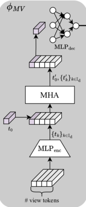
Figure 7: Attention Layer. We additionally investigated Multi-Head-Attention (MHA) layers to fuse geometry information from multiple images. As another method of aggregating multi-views, the Multi-Head self-At, replacing the $\Phi_{MV}$ in Fig. 2. Fig. 10 shows qualitative results with using the attention layers for multi-view aggregation.

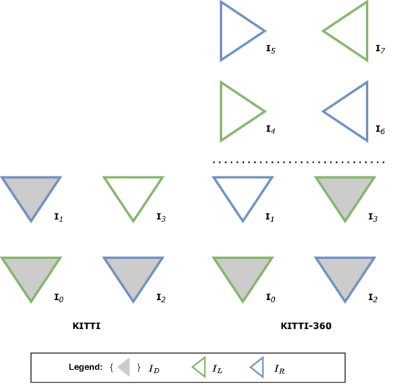
Figure 8: Frame Arrangement in temporal steps. The possible frames are split into either loss set $I_{L}$ or render loss set $I_{R}$. Note that the first frame starting with zero index is used for an input frame as fixed. Both KITTI-360 and KITTI use stereo cameras. Depending on the experiments’ setup, having fisheyes as input scenes is optional. This influence has been discussed in the ablation study of the main paper.

7.2 Occupancy Estimation

Fig. 9 shows the occupancy accuracy for Knowledge-Distillation Behind the Scenes (KDBTS) and BTS for different depth values. The performance increase of KDBTS mainly happens at depth values larger than $10$ meters.

Tab. 5 to Tab. 9 gives the complete overview of the settings tested in the ablation study of the main paper for five different camera settings at inference time. The different setups used in these tables are illustrated in Fig. 11. It shows the general improvement of all models tested in the ablation study when providing more frames at inference time, except for the model with attention layers. Our model performs best in all settings with a few minor exceptions. We additionally show the influence of including fisheye cameras at inference time in Tab. 9.

Figure 9: Occupancy Accuracy At Different Depths. KDBTS shows on par performance for occupancy estimation to BTS for depth values (z) smaller than $10$ m. For depths larger than $10$ m, KDBTS starts to outperform BTS significantly.

7.3 Occupancy profiles

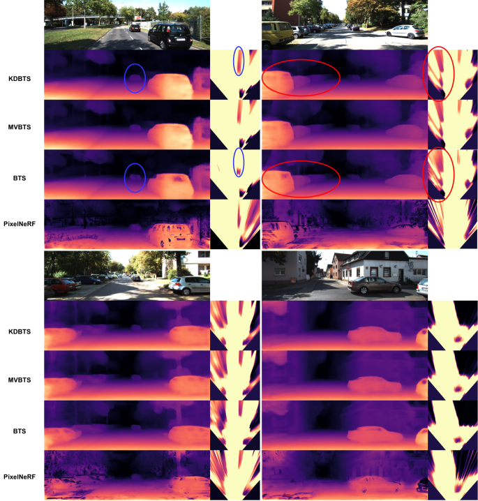
Figure 13: Qualitative Baseline Results 1. Baselines comparison in both depth- and occupancy estimation. The camera frustum is set up in x=[-9, 9]m, y=[0, 0.75]m, and z=[3,21]m. It shows general improvements by our methods, such as removing occupancy behind parked cars, leading to cleaner occupancy predictions (see top right example). The top left shows a failure case of our method where a moving car produces a drawn-out shadow for our methods, likely resulting from conflicting temporal information.

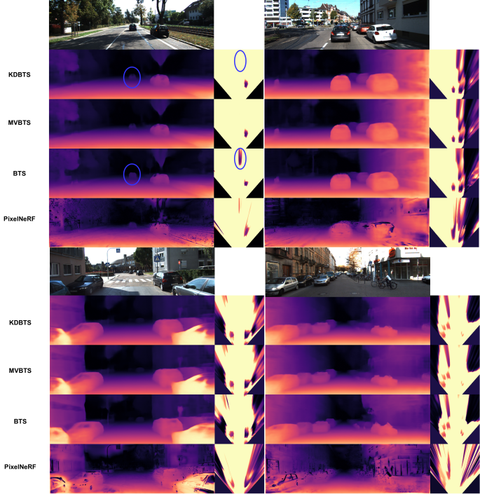
Figure 14: Qualitative Baseline Results 2. Baselines comparison in both depth- and occupancy estimation. The camera frustum is set up in x=[-9, 9]m, y=[0, 0.75]m, and z=[3,21]m. Our method shows general improvements, such as removing holes in car windows (see lower examples) or predicting the house facades to be in a straight line (see lower right example). It also shows a failure case (top left) where our methods remove a moving car from the scene, likely due to conflicting temporal information.

We present additional visualizations of our models and the baselines BTS [52] and PixelNeRF [56] in Fig. 13 and Fig. 14 in the monocular occupancy prediction setting. The examples show overall improvements in our scene reconstruction. Our models produce cleaner edges and show a better holistic scene understanding by reconstructing house facades as straight lines, removing some of the bulges in BTS. Apart from the overall improvements of our approach compared to BTS, they also demonstrate some of the limitations of the static scene assumption taken in our model. Dynamic objects in the scene can lead to conflicting information in the scene reconstruction of our MVBTS model, which also affects KDBTS. This results in either drawn-out shadows of dynamic objects (see the first example of Fig. 13) or our models removing the dynamic object entirely (see the first example of Fig. 14).

7.4 Depth Prediction

We evaluate the depth predictions generated by our models compared to established baselines such as BTS [52] and PixelNeRF [56], specifically focusing on monocular input.

Figures 13 and 14 visually present the depth predictions obtained from our models and the aforementioned baselines. Our models demonstrate performance on par with BTS in terms of overall accuracy. However, a notable difference lies in the prediction of car windows, where our models tend to exhibit fewer holes compared to BTS. Conversely, our models may show slightly increased blur at the edges of reconstructed objects.

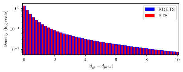
(a) absolute error distribution.

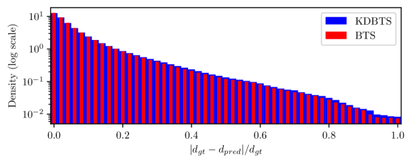
(b) relative error distribution.

Figure 12: Depth Prediction Error Distributions. The error distributions are similar for both methods - KDBTS has slightly more large errors than BTS. Lower errors for KDBTS (blue dots) and BTS (red dots), intensity encodes magnitude. Qualitative examples (see Fig. 15) for the depth error on the KITTI test set show that KDTBS often performs worse on dynamic objects (e.g. cars, cyclists).

To further analyze the performance differences, we examine the error distribution depicted in Fig. 12. While the majority of errors appear similar between our model (KDBTS) and BTS, KDBTS tends to exhibit more large errors, indicating the violation of static scene assumption.

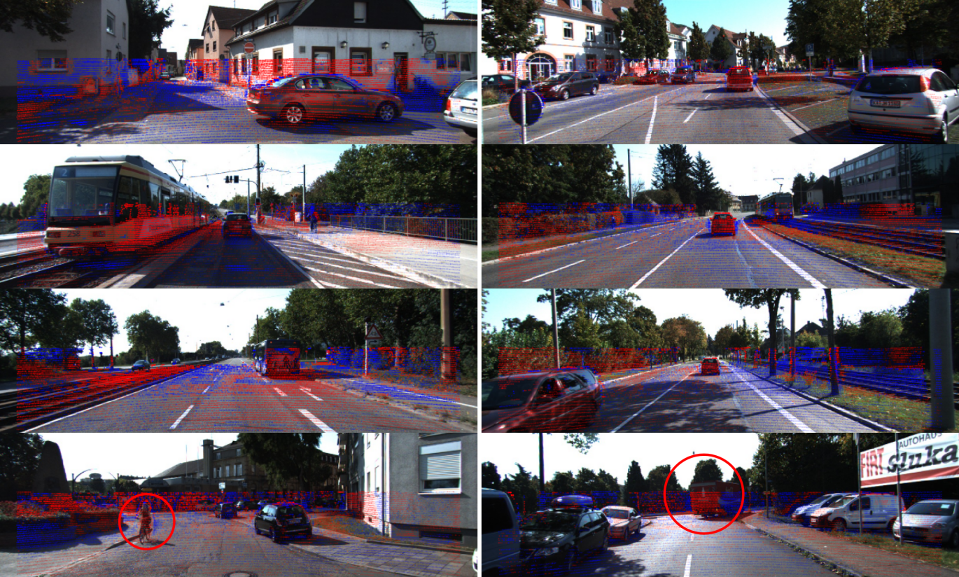
Figure 15: Depth error comparison between BTS and KDBTS. KDBTS exhibits slightly more large errors compared to BTS. Qualitative examples (bottom) demonstrate depth error on the KITTI test set, with lower errors depicted by KDBTS (blue dots) and BTS (red dots), with intensity representing magnitude. Each test image presents the projected scene from the LiDAR ground truth point cloud. The projected LiDAR point cloud is used to calculate the distance error between the prediction and its ground truth. Color differentiation indicates lesser distance errors between KDBTS (blue dots) and BTS (red dots). In KDBTS, the model’s reconstruction is affected by moving objects, resulting in larger errors typically observed on dynamic objects (e.g., cars, cyclists). Consequently, red dots are depicted for dynamic objects, signifying lower errors for BTS.

In Fig. 15, we provide a qualitative comparison of the depth predictions generated by KDBTS and BTS. Although both methods perform comparably overall, KDBTS shows a tendency to perform worse, particularly in scenarios involving dynamic objects. This discrepancy is attributed to violations of the static scene assumption, where the prediction of moving cars may vanish due to conflicting information from multiple time steps (as illustrated in Fig. 14). These inconsistencies in temporal information impact the reconstruction quality, affecting both depth and occupancy estimates.

8 Implementation Details

In the following, we detail the implementation details of our method, including the network architecture and training hyperparameters. For additional details, such as more information about the rendering process and the positional encoding, we refer the reader to [52] and its supplementary material.

8.1 Network Architecture

For implementation reasons, our network consists of a backbone encoder-decoder network and two decoder networks for both the single-view and multi-view settings, respectively.

Backbone. For the backbone, we follow Monodepth2 [13] and BTS [52] such that the reported results stem from the different training setups. It is comprised of a ResNet50 network [19] with an adjustable channel size of 64. As with BTS [52], there is no feature reduction in the upconvolutions of the network.

Single-View Head. The single-view decoding network follows [52] exactly and is comprised of a layer-connected network with ReLU activation functions and residual connections. The input dimension of the MLP is $103$ ($64$ feature channel size + $39$ positional encoding size) and the network has a hidden dimension of $64$.

Multi-View Head. The multi-view decoding network consists of two MLPs with the same architecture as the single-view decoding network. $\text{MLP}_{1}$, acting as a feature reduction network, has an input dimension of $103$, a hidden dimension of $128$, and an output size of $17$ ($1$ confidence value + $16$ feature channel size). $\text{MLP}_{2}$ has an input dimension of $16$, and a hidden dimension of $16$. The softmax layer in between the MLPs uses no temperature scaling.

Ablation Study Network. For our ablation study, we also test networks where the MLP dimensions are set to the following for the large network:

• $\text{MLP}_{1}$ (input: $103$, hidden: $256$, output: $33$)

• $\text{MLP}_{2}$ (input: $32$, hidden: $32$, output: $1$)

and to

• $\text{MLP}_{1}$ (input: $103$, hidden: $128$, output: $2$)

• no $\text{MLP}_{2}$

for the small model. The small network does not do feature fusion but rather directly fuses the different frames’ density prediction.

8.2 Training Configuration

Hyperparameters For training on both KITTI [11] and KITTI-360 [32], we use the same set of hyperparameters. We use a batch size of $8$ during training. We use the patched-based sampling strategy of [52] and sample $32$ random patches of size $8\times 8$, giving us $2048$ rays in total per batch. The loss weights are set to $\lambda_{SSIM}=0.85$, $\lambda_{\text{L1}}=0.15$ following [52, 13] and $\lambda_{\text{EAS}}=10^{-3}$ following the code implementation of [52]. We use an ADAM optimizer with a learning rate of $\lambda=10^{-4}$ for the first 120,000 steps and $\lambda=10^{-5}$ for the rest. We apply the same color augmentation and random flips as [52]. For our knowledge distillation, we train with a constant learning rate of $\lambda=10^{-4}$.

Figure 10: Attention Layer Qualitative Results. Comparison in both depth- and occupancy estimation. The camera frustum is set up in x=[-9, 9]m, y=[0, 0.75]m, and z=[3,21]m. The monocular occupancy prediction produces reasonable results for both the expected ray termination depth and the occupancy profiles. Adding more frames to the prediction leads to increased noise in the predictions. A closer inspection of the occupancy profiles shows that the attention model produces long and thin occupancy shadows along rays cast from the camera. The occupancy predictions seem to be quite sensitive to changes in the features coming from the pixel-aligned feature map.

Figure 11: Frame Arrangement in Inference. Illustration of the settings used at inference time in Tab. 5, Tab. 6, Tab. 7, Tab. 8, and Tab. 9.

Inference	dropout	MLPs	attn. layers	encode fisheye	$\text{O}_{\text{acc}}\uparrow$	$\text{O}_{\text{prec}}\uparrow$	$\text{O}_{\text{rec}}\uparrow$	$\text{IE}_{\text{acc}}\uparrow$	$\text{IE}_{\text{prec}}\uparrow$	$\text{IE}_{\text{rec}}\uparrow$
(Mono)	0.5	middle	✓	✗	93.98%	57.41%	80.47%	74.43%	48.40%	44.47%
(Mono)	0.0	middle	✗	✓	93.81%	57.07%	82.60%	73.03%	50.55%	39.54%
(Mono)	0.2	middle	✗	✓	94.37%	59.03%	80.91%	76.24%	51.06%	46.28%
(Mono)	0.5	middle	✗	✓	94.71%	60.31%	83.35%	77.89%	52.96%	46.02%
(Mono)	0.8	middle	✗	✓	94.78%	60.09%	85.38%	77.76%	53.25%	43.43%
(Mono)	0.5	small	✗	✗	94.51%	59.62%	85.18%	76.88%	52.80%	40.80%
(Mono)	0.5	large	✗	✗	94.16%	58.56%	80.96%	76.04%	50.78%	46.69%
(Mono)	0.5	middle	✗	✗	94.76%	60.83%	84.51%	78.00%	53.69%	44.04%

Table 5: Ablation Studies in Monocular Inference. Evaluation of all models in the ablations study in the monocular setting (see Fig. 11 for more details of the frame arrangements). As for the setting in the main paper, our final architecture performs the best with a few exceptions. The model with more dropout performs slightly better in the occupancy estimation task. This is likely due to having fewer frames available during training. Additionally, some of the methods that also encoded fisheye cameras during training as well perform better when it comes to the $\text{IE}_{rec}$ but worse at $\text{IE}_{prec}$. They produce fewer false negatives, but more false positives, meaning less space is predicted as being empty.

Inference	dropout	MLPs	attn. layers	encode fisheye	$\text{O}_{\text{acc}}\uparrow$	$\text{O}_{\text{prec}}\uparrow$	$\text{O}_{\text{rec}}\uparrow$	$\text{IE}_{\text{acc}}\uparrow$	$\text{IE}_{\text{prec}}\uparrow$	$\text{IE}_{\text{rec}}\uparrow$
(M+T)	0.5	middle	✓	✗	93.79%	58.97%	77.44%	72.93%	45.81%	47.91%
(M+T)	0.0	middle	✗	✓	93.69%	57.36%	81.59%	73.50%	45.66%	41.07%
(M+T)	0.2	middle	✗	✓	94.42%	59.45%	81.76%	76.45%	51.44%	45.94%
(M+T)	0.5	middle	✗	✓	94.78%	60.69%	84.37%	77.93%	55.32%	45.81%
(M+T)	0.8	middle	✗	✓	94.90%	60.42%	86.04%	79.21%	53.55%	43.73%
(M+T)	0.5	small	✗	✗	94.56%	59.95%	85.98%	78.37%	55.30%	42.65%
(M+T)	0.5	large	✗	✗	94.30%	59.21%	81.28%	76.65%	50.74%	47.85%
(M+T)	0.5	middle	✗	✗	94.82%	61.02%	84.83%	78.73%	53.88%	44.81%

Table 6: Ablation Studies in Temporal Monocular Inference. Using one additional temporal frame shows slight improvements for all methods, with the exception of the attention layer model (see Fig. 11 for more details of the frame setup). Otherwise, the difference between the models is similar to the monocular setting. The model with a higher dropout gains additional performance improvements to our final model.

Inference	dropout	MLPs	attn. layers	encode fisheye	$\text{O}_{\text{acc}}\uparrow$	$\text{O}_{\text{prec}}\uparrow$	$\text{O}_{\text{rec}}\uparrow$	$\text{IE}_{\text{acc}}\uparrow$	$\text{IE}_{\text{prec}}\uparrow$	$\text{IE}_{\text{rec}}\uparrow$
(S)	0.5	middle	✓	✗	93.92%	59.26%	78.57%	73.34%	45.11%	47.37%
(S)	0.0	middle	✗	✓	93.41%	57.21%	80.23%	72.40%	46.38%	42.14%
(S)	0.2	middle	✗	✓	94.53%	59.02%	82.04%	76.65%	53.67%	45.97%
(S)	0.5	middle	✗	✓	94.87%	60.09%	84.58%	78.37%	54.75%	45.71%
(S)	0.8	middle	✗	✓	94.89%	60.07%	85.64%	77.98%	54.12%	43.22%
(S)	0.5	small	✗	✗	94.56%	59.34%	86.20%	77.92%	54.36%	42.44%
(S)	0.5	large	✗	✗	94.29%	58.86%	81.83%	76.15%	50.90%	46.15%
(S)	0.5	middle	✗	✗	94.84%	61.12%	85.28%	78.62%	54.02%	44.05%

Table 7: Ablation Studies in Stereo Inference. Using stereo frame also shows slight improvements for all methods, with the exception of the attention layer model (see Fig. 11 for more details of the frame setup).

Inference	dropout	MLPs	attn. layers	encode fisheye	$\text{O}_{\text{acc}}\uparrow$	$\text{O}_{\text{prec}}\uparrow$	$\text{O}_{\text{rec}}\uparrow$	$\text{IE}_{\text{acc}}\uparrow$	$\text{IE}_{\text{prec}}\uparrow$	$\text{IE}_{\text{rec}}\uparrow$
(S + T)	0.5	middle	✓	✗	93.23%	60.77%	70.69%	69.83%	47.40%	58.94%
(S + T)	0.0	middle	✗	✓	93.44%	56.85%	79.74%	73.02%	45.54%	43.90%
(S + T)	0.2	middle	✗	✓	94.57%	59.85%	83.20%	77.13%	54.41%	45.64%
(S + T)	0.5	middle	✗	✓	94.93%	60.72%	85.47%	79.05%	55.73%	46.39%
(S + T)	0.8	middle	✗	✓	94.94%	60.43%	86.40%	79.41%	55.35%	44.80%
(S + T)	0.5	small	✗	✗	94.64%	59.64%	86.65%	78.54%	55.04%	43.70%
(S + T)	0.5	large	✗	✗	94.38%	59.88%	82.51%	77.24%	51.66%	46.90%
(S + T)	0.5	middle	✗	✗	94.91%	61.73%	85.78%	79.47%	55.08%	45.23%

Table 8: Ablation Studies in Temporal Stereo Inference. For convenience, we repeat the findings of the main paper here (see Fig. 11 for more details of the frame setup).

Inference	dropout	MLPs	attn. layers	encode fisheye	$\text{O}_{\text{acc}}\uparrow$	$\text{O}_{\text{prec}}\uparrow$	$\text{O}_{\text{rec}}\uparrow$	$\text{IE}_{\text{acc}}\uparrow$	$\text{IE}_{\text{prec}}\uparrow$	$\text{IE}_{\text{rec}}\uparrow$
(S+T+F)	0.5	middle	✓	✗	92.88%	58.51%	71.39%	69.67%	47.31%	57.28%
(S+T+F)	0.0	middle	✗	✓	93.22%	55.79%	78.58%	72.36%	44.49%	44.09%
(S+T+F)	0.2	middle	✗	✓	94.54%	58.77%	84.05%	77.19%	55.16%	44.00%
(S+T+F)	0.5	middle	✗	✓	94.90%	60.34%	85.31%	78.84%	56.08%	46.04%
(S+T+F)	0.8	middle	✗	✓	94.91%	60.23%	86.22%	79.31%	55.22%	44.50%
(S+T+F)	0.5	small	✗	✗	94.67%	59.17%	86.65%	78.54%	54.97%	43.45%
(S+T+F)	0.5	large	✗	✗	94.38%	59.22%	82.68%	77.08%	51.53%	45.90%
(S+T+F)	0.5	middle	✗	✗	94.89%	60.38%	85.83%	79.44%	55.30%	44.90%

Table 9: Ablation Studies in Temporal Stereo Fisheye Inference. Using the fisheye cameras for inference does not give large improvements for all methods. This shows that a lot of the scene information can already be captured in the pinhole frames alone (see Fig. 11 for more details of the frame setup).

References

- Buehler et al. [2001] Chris Buehler, Michael Bosse, Leonard McMillan, Steven Gortler, and Michael Cohen. Unstructured lumigraph rendering. SIGGRAPH, 2001.
- Cai et al. [2021] Yingjie Cai, Xuesong Chen, Chao Zhang, Kwan-Yee Lin, Xiaogang Wang, and Hongsheng Li. Semantic scene completion via integrating instances and scene in-the-loop. In Proceedings of the IEEE/CVF Conference on Computer Vision and Pattern Recognition, pages 324–333, 2021.
- Campos et al. [2021] Carlos Campos, Richard Elvira, Juan J Gómez Rodríguez, José MM Montiel, and Juan D Tardós. Orb-slam3: An accurate open-source library for visual, visual–inertial, and multimap slam. IEEE Transactions on Robotics, 37(6):1874–1890, 2021.
- Cao and de Charette [2022] Anh-Quan Cao and Raoul de Charette. Monoscene: Monocular 3d semantic scene completion. In CVPR, 2022.
- Chen et al. [2020] Xiaokang Chen, Kwan-Yee Lin, Chen Qian, Gang Zeng, and Hongsheng Li. 3d sketch-aware semantic scene completion via semi-supervised structure prior. In Proceedings of the IEEE/CVF Conference on Computer Vision and Pattern Recognition, pages 4193–4202, 2020.
- Cheng et al. [2021] Ran Cheng, Christopher Agia, Yuan Ren, Xinhai Li, and Liu Bingbing. S3cnet: A sparse semantic scene completion network for lidar point clouds. In Conference on Robot Learning, pages 2148–2161. PMLR, 2021.
- Davis et al. [2012] Abe Davis, Marc Levoy, and Fredo Durand. Unstructured light fields. In Computer Graphics Forum, pages 305–314. Wiley Online Library, 2012.
- Debevec et al. [1996] Paul E Debevec, Camillo J Taylor, and Jitendra Malik. Modeling and rendering architecture from photographs: A hybrid geometry-and image-based approach. Computer graphics and interactive techniques, 1996.
- Eigen et al. [2014] David Eigen, Christian Puhrsch, and Rob Fergus. Depth map prediction from a single image using a multi-scale deep network. Advances in neural information processing systems, 27, 2014.
- Firman et al. [2016] Michael Firman, Oisin Mac Aodha, Simon Julier, and Gabriel J Brostow. Structured prediction of unobserved voxels from a single depth image. In Proceedings of the IEEE Conference on Computer Vision and Pattern Recognition, pages 5431–5440, 2016.
- Geiger et al. [2013] Andreas Geiger, Philip Lenz, Christoph Stiller, and Raquel Urtasun. Vision meets robotics: The kitti dataset. The International Journal of Robotics Research, 32(11):1231–1237, 2013.
- Godard et al. [2017] Clément Godard, Oisin Mac Aodha, and Gabriel J Brostow. Unsupervised monocular depth estimation with left-right consistency. In Proceedings of the IEEE conference on computer vision and pattern recognition, pages 270–279, 2017.
- Godard et al. [2019] Clément Godard, Oisin Mac Aodha, Michael Firman, and Gabriel J Brostow. Digging into self-supervised monocular depth estimation. In Proceedings of the IEEE/CVF International Conference on Computer Vision, pages 3828–3838, 2019.
- GonzalezBello and Kim [2020] Juan Luis GonzalezBello and Munchurl Kim. Forget about the lidar: Self-supervised depth estimators with med probability volumes. Advances in Neural Information Processing Systems, 33:12626–12637, 2020.
- Gortler et al. [1996] Steven J. Gortler, Radek Grzeszczuk, Richard Szeliski, and Michael F. Cohen. The lumigraph. In Proceedings of the 23rd Annual Conference on Computer Graphics and Interactive Techniques, 1996.
- Guizilini et al. [2020] Vitor Guizilini, Rares Ambrus, Sudeep Pillai, Allan Raventos, and Adrien Gaidon. 3d packing for self-supervised monocular depth estimation. In Proceedings of the IEEE/CVF Conference on Computer Vision and Pattern Recognition, pages 2485–2494, 2020.
- Harris and Stephens [1988] C. Harris and M. Stephens. A combined corner and edge detector. In Proceedings of the 4th Alvey Vision Conference, 1988.
- Hayler et al. [2023] Adrian Hayler, Felix Wimbauer, Dominik Muhle, Christian Rupprecht, and Daniel Cremers. S4c: Self-supervised semantic scene completion with neural fields. arXiv preprint arXiv:2310.07522, 2023.
- He et al. [2015] Kaiming He, Xiangyu Zhang, Shaoqing Ren, and Jian Sun. Deep residual learning for image recognition, 2015.
- He et al. [2016] Kaiming He, Xiangyu Zhang, Shaoqing Ren, and Jian Sun. Deep residual learning for image recognition. In Proceedings of the IEEE conference on computer vision and pattern recognition, pages 770–778, 2016.
- Heigl et al. [1999] Benno Heigl, Reinhard Koch, Marc Pollefeys, Joachim Denzler, and Luc J. Van Gool. Plenoptic modeling and rendering from image sequences taken by hand-held camera. In Mustererkennung 1999, 21. DAGM-Symposium, 1999.
- Irshad et al. [2023] Muhammad Zubair Irshad, Sergey Zakharov, Katherine Liu, Vitor Guizilini, Thomas Kollar, Adrien Gaidon, Zsolt Kira, and Rares Ambrus. Neo 360: Neural fields for sparse view synthesis of outdoor scenes. In ICCV, 2023.
- Johari et al. [2022] M. Johari, Y. Lepoittevin, and F. Fleuret. Geonerf: Generalizing nerf with geometry priors. In Proceedings of the IEEE International Conference on Computer Vision and Pattern Recognition (CVPR), 2022.
- Khamis et al. [2018] Sameh Khamis, Sean Fanello, Christoph Rhemann, Adarsh Kowdle, Julien Valentin, and Shahram Izadi. Stereonet: Guided hierarchical refinement for real-time edge-aware depth prediction. In Proceedings of the European Conference on Computer Vision (ECCV), 2018.
- Koestler et al. [2022] Lukas Koestler, Nan Yang, Niclas Zeller, and Daniel Cremers. Tandem: Tracking and dense mapping in real-time using deep multi-view stereo. In Conference on Robot Learning, pages 34–45. PMLR, 2022.
- Li et al. [2019a] Jie Li, Yu Liu, Dong Gong, Qinfeng Shi, Xia Yuan, Chunxia Zhao, and Ian Reid. Rgbd based dimensional decomposition residual network for 3d semantic scene completion. In Proceedings of the IEEE/CVF Conference on Computer Vision and Pattern Recognition, pages 7693–7702, 2019a.
- Li et al. [2019b] Jie Li, Yu Liu, Xia Yuan, Chunxia Zhao, Roland Siegwart, Ian Reid, and Cesar Cadena. Depth based semantic scene completion with position importance aware loss. IEEE Robotics and Automation Letters, 5(1):219–226, 2019b.
- Li et al. [2020] Jie Li, Kai Han, Peng Wang, Yu Liu, and Xia Yuan. Anisotropic convolutional networks for 3d semantic scene completion. In Proceedings of the IEEE/CVF Conference on Computer Vision and Pattern Recognition, pages 3351–3359, 2020.
- Li et al. [2021a] Jiaxin Li, Zijian Feng, Qi She, Henghui Ding, Changhu Wang, and Gim Hee Lee. Mine: Towards continuous depth mpi with nerf for novel view synthesis. In Proceedings of the IEEE/CVF International Conference on Computer Vision, pages 12578–12588, 2021a.
- Li et al. [2021b] Pengfei Li, Yongliang Shi, Tianyu Liu, Hao Zhao, Guyue Zhou, and Ya-Qin Zhang. Semi-supervised implicit scene completion from sparse lidar, 2021b.
- Li et al. [2023] Yiming Li, Zhiding Yu, Christopher Choy, Chaowei Xiao, Jose M Alvarez, Sanja Fidler, Chen Feng, and Anima Anandkumar. Voxformer: Sparse voxel transformer for camera-based 3d semantic scene completion. In CVPR, 2023.
- Liao et al. [2022] Yiyi Liao, Jun Xie, and Andreas Geiger. Kitti-360: A novel dataset and benchmarks for urban scene understanding in 2d and 3d. IEEE Transactions on Pattern Analysis and Machine Intelligence, 2022.
- Liu et al. [2018] Shice Liu, Yu Hu, Yiming Zeng, Qiankun Tang, Beibei Jin, Yinhe Han, and Xiaowei Li. See and think: Disentangling semantic scene completion. In Advances in Neural Information Processing Systems, 2018.
- Liu et al. [2022] Yuan Liu, Sida Peng, Lingjie Liu, Qianqian Wang, Peng Wang, Christian Theobalt, Xiaowei Zhou, and Wenping Wang. Neural rays for occlusion-aware image-based rendering. In CVPR, 2022.
- Lowe [2004] David G Lowe. Distinctive image features from scale-invariant keypoints. International journal of computer vision, 60:91–110, 2004.
- Luo et al. [2019] Chenxu Luo, Zhenheng Yang, Peng Wang, Yang Wang, Wei Xu, Ram Nevatia, and Alan Yuille. Every pixel counts++: Joint learning of geometry and motion with 3d holistic understanding. IEEE transactions on pattern analysis and machine intelligence, 42(10):2624–2641, 2019.
- Lyu et al. [2021] Xiaoyang Lyu, Liang Liu, Mengmeng Wang, Xin Kong, Lina Liu, Yong Liu, Xinxin Chen, and Yi Yuan. Hr-depth: High resolution self-supervised monocular depth estimation. In AAAI, pages 2294–2301, 2021.
- Mildenhall et al. [2021] Ben Mildenhall, Pratul P Srinivasan, Matthew Tancik, Jonathan T Barron, Ravi Ramamoorthi, and Ren Ng. Nerf: Representing scenes as neural radiance fields for view synthesis. Communications of the ACM, 65(1):99–106, 2021.
- Niemeyer et al. [2022] Michael Niemeyer, Jonathan T Barron, Ben Mildenhall, Mehdi SM Sajjadi, Andreas Geiger, and Noha Radwan. Regnerf: Regularizing neural radiance fields for view synthesis from sparse inputs. In Proceedings of the IEEE/CVF Conference on Computer Vision and Pattern Recognition, pages 5480–5490, 2022.
- Rist et al. [2021] Christoph B Rist, David Emmerichs, Markus Enzweiler, and Dariu M Gavrila. Semantic scene completion using local deep implicit functions on lidar data. IEEE transactions on pattern analysis and machine intelligence, 44(10):7205–7218, 2021.
- Roldao et al. [2020] Luis Roldao, Raoul de Charette, and Anne Verroust-Blondet. Lmscnet: Lightweight multiscale 3d semantic completion. In 2020 International Conference on 3D Vision (3DV), 2020.
- Rublee et al. [2011] Ethan Rublee, Vincent Rabaud, Kurt Konolige, and Gary Bradski. Orb: An efficient alternative to sift or surf. In 2011 International conference on computer vision, pages 2564–2571. Ieee, 2011.
- Schönberger and Frahm [2016] Johannes Lutz Schönberger and Jan-Michael Frahm. Structure-from-motion revisited. In Conference on Computer Vision and Pattern Recognition (CVPR), 2016.
- Sharma et al. [2023] Prafull Sharma, Ayush Tewari, Yilun Du, Sergey Zakharov, Rares Andrei Ambrus, Adrien Gaidon, William T. Freeman, Fredo Durand, Joshua B. Tenenbaum, and Vincent Sitzmann. Neural groundplans: Persistent neural scene representations from a single image. In The Eleventh International Conference on Learning Representations, 2023.
- Shu et al. [2020] Chang Shu, Kun Yu, Zhixiang Duan, and Kuiyuan Yang. Feature-metric loss for self-supervised learning of depth and egomotion. In European Conference on Computer Vision, pages 572–588. Springer, 2020.
- Song et al. [2017] Shuran Song, Fisher Yu, Andy Zeng, Angel X Chang, Manolis Savva, and Thomas Funkhouser. Semantic scene completion from a single depth image. In Proceedings of the IEEE conference on computer vision and pattern recognition, pages 1746–1754, 2017.
- Spencer et al. [2020] Jaime Spencer, Richard Bowden, and Simon Hadfield. Defeat-net: General monocular depth via simultaneous unsupervised representation learning. In CVPR, pages 14402–14413, 2020.
- Verbin et al. [2022] Dor Verbin, Peter Hedman, Ben Mildenhall, Todd Zickler, Jonathan T Barron, and Pratul P Srinivasan. Ref-nerf: Structured view-dependent appearance for neural radiance fields. In 2022 IEEE/CVF Conference on Computer Vision and Pattern Recognition (CVPR), pages 5481–5490. IEEE, 2022.
- Wang et al. [2021] Qianqian Wang, Zhicheng Wang, Kyle Genova, Pratul Srinivasan, Howard Zhou, Jonathan T. Barron, Ricardo Martin-Brualla, Noah Snavely, and Thomas Funkhouser. Ibrnet: Learning multi-view image-based rendering. In CVPR, 2021.
- Watson et al. [2019] Jamie Watson, Michael Firman, Gabriel J Brostow, and Daniyar Turmukhambetov. Self-supervised monocular depth hints. In Proceedings of the IEEE/CVF International Conference on Computer Vision, pages 2162–2171, 2019.
- Wimbauer et al. [2021] Felix Wimbauer, Nan Yang, Lukas Von Stumberg, Niclas Zeller, and Daniel Cremers. Monorec: Semi-supervised dense reconstruction in dynamic environments from a single moving camera. In Proceedings of the IEEE/CVF Conference on Computer Vision and Pattern Recognition, pages 6112–6122, 2021.
- Wimbauer et al. [2023] Felix Wimbauer, Nan Yang, Christian Rupprecht, and Daniel Cremers. Behind the scenes: Density fields for single view reconstruction. In Proceedings of the IEEE/CVF Conference on Computer Vision and Pattern Recognition, pages 9076–9086, 2023.
- Wu et al. [2015] Zhirong Wu, Shuran Song, Aditya Khosla, Fisher Yu, Linguang Zhang, Xiaoou Tang, and Jianxiong Xiao. 3d shapenets: A deep representation for volumetric shapes. In Proceedings of the IEEE conference on computer vision and pattern recognition, pages 1912–1920, 2015.
- Yan et al. [2021] Xu Yan, Jiantao Gao, Jie Li, Ruimao Zhang, Zhen Li, Rui Huang, and Shuguang Cui. Sparse single sweep lidar point cloud segmentation via learning contextual shape priors from scene completion. In Proceedings of the AAAI Conference on Artificial Intelligence, pages 3101–3109, 2021.
- Yang et al. [2018] Nan Yang, Rui Wang, Jorg Stuckler, and Daniel Cremers. Deep virtual stereo odometry: Leveraging deep depth prediction for monocular direct sparse odometry. In Proceedings of the European Conference on Computer Vision (ECCV), pages 817–833, 2018.
- Yu et al. [2021] Alex Yu, Vickie Ye, Matthew Tancik, and Angjoo Kanazawa. pixelnerf: Neural radiance fields from one or few images. In Proceedings of the IEEE/CVF Conference on Computer Vision and Pattern Recognition, pages 4578–4587, 2021.
- Yuan et al. [2022] Weihao Yuan, Xiaodong Gu, Zuozhuo Dai, Siyu Zhu, and Ping Tan. New crfs: Neural window fully-connected crfs for monocular depth estimation. arXiv preprint arXiv:2203.01502, 2022.
- Zhan et al. [2018] Huangying Zhan, Ravi Garg, Chamara Saroj Weerasekera, Kejie Li, Harsh Agarwal, and Ian Reid. Unsupervised learning of monocular depth estimation and visual odometry with deep feature reconstruction. In Proceedings of the IEEE conference on computer vision and pattern recognition, pages 340–349, 2018.
- Zhang et al. [2019a] Feihu Zhang, Victor Prisacariu, Ruigang Yang, and Philip HS Torr. Ga-net: Guided aggregation net for end-to-end stereo matching. In Proceedings of the IEEE/CVF Conference on Computer Vision and Pattern Recognition, pages 185–194, 2019a.
- Zhang et al. [2018] Jiahui Zhang, Hao Zhao, Anbang Yao, Yurong Chen, Li Zhang, and Hongen Liao. Efficient semantic scene completion network with spatial group convolution. In Proceedings of the European Conference on Computer Vision (ECCV), pages 733–749, 2018.
- Zhang et al. [2019b] Pingping Zhang, Wei Liu, Yinjie Lei, Huchuan Lu, and Xiaoyun Yang. Cascaded context pyramid for full-resolution 3d semantic scene completion. In Proceedings of the IEEE/CVF International Conference on Computer Vision, pages 7801–7810, 2019b.
- Zhou et al. [2021] Hang Zhou, David Greenwood, and Sarah Taylor. Self-supervised monocular depth estimation with internal feature fusion. In BMVC, 2021.
- Zhou et al. [2022] Kaichen Zhou, Lanqing Hong, Changhao Chen, Hang Xu, Chaoqiang Ye, Qingyong Hu, and Zhenguo Li. Devnet: Self-supervised monocular depth learning via density volume construction. arXiv preprint arXiv:2209.06351, 2022.
- Zhou et al. [2017] Tinghui Zhou, Matthew Brown, Noah Snavely, and David G Lowe. Unsupervised learning of depth and ego-motion from video. In Proceedings of the IEEE conference on computer vision and pattern recognition, pages 1851–1858, 2017.