FusionMamba: Efficient Image Fusion with State Space Model

Abstract.

Image fusion aims to generate a high-resolution multi/hyper-spectral image by combining a high-resolution image with limited spectral information and a low-resolution image with abundant spectral data. Current deep learning (DL)-based methods for image fusion primarily rely on CNNs or Transformers to extract features and merge different types of data. While CNNs are efficient, their receptive fields are limited, restricting their capacity to capture global context. Conversely, Transformers excel at learning global information but are hindered by their quadratic complexity. Fortunately, recent advancements in the State Space Model (SSM), particularly Mamba, offer a promising solution to this issue by enabling global awareness with linear complexity. However, there have been few attempts to explore the potential of SSM in information fusion, which is a crucial ability in domains like image fusion. Therefore, we propose FusionMamba, an innovative method for efficient image fusion. Our contributions mainly focus on two aspects. Firstly, recognizing that images from different sources possess distinct properties, we incorporate Mamba blocks into two U-shaped networks, presenting a novel architecture that extracts spatial and spectral features in an efficient, independent, and hierarchical manner. Secondly, to effectively combine spatial and spectral information, we extend the Mamba block to accommodate dual inputs. This expansion leads to the creation of a new module called the FusionMamba block, which outperforms existing fusion techniques such as concatenation and cross-attention. To validate FusionMamba’s effectiveness, we conduct a series of experiments on five datasets related to three image fusion tasks. The quantitative and qualitative evaluation results demonstrate that our method achieves state-of-the-art (SOTA) performance, underscoring the superiority of FusionMamba.

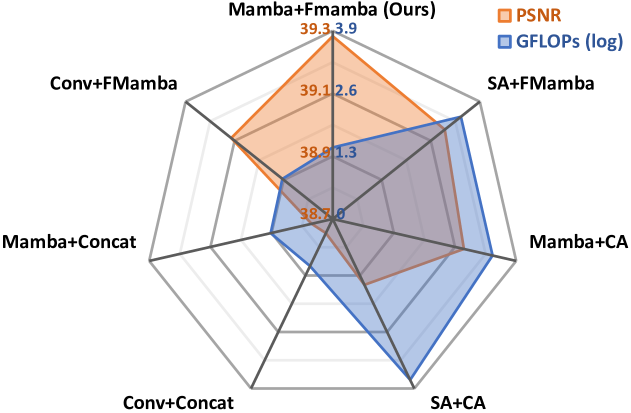
Figure 1. Performance and efficiency comparisons among different combinations of network components. The feature extraction modules being compared are convolution (Conv), self-attention (SA), and the Mamba block. Additionally, the information fusion modules include concatenation (Concat), cross-attention (CA), and the proposed FusionMamba block (FMamba). With identical parameter counts, our method demonstrates superior performance while maintaining a reasonable level of FLOP consumption. Dataset: WV3.

1. Introduction

Because of hardware constraints, sensors are unable to directly acquire high-resolution multi/hyper-spectral images. Instead, they can simultaneously capture a high-resolution image with limited spectral information and a low-resolution image with abundant spectral data. Image fusion seeks to combine these two types of images to generate a high-resolution result with rich spectral information. This work focuses on three image fusion tasks: pansharpening, hyper-spectral pansharpening, and hyper-spectral image super-resolution (HISR). Pansharpening combines a panchromatic (PAN) image with a low-resolution multi-spectral (LRMS) image to create a high-resolution multi-spectral (HRMS) result. Hyper-spectral pansharpening involves generating a high-resolution hyper-spectral (HRHS) image from a PAN image and a low-resolution hyper-spectral (LRHS) image. Lastly, HISR aims to produce an HRHS image by merging an RGB image with an LRHS image.

Traditional image fusion approaches aim at revealing the intrinsic relationships between two types of images. They typically rely on different forms of prior information to construct optimization models for combining spatial and spectral data (Palsson et al., 2013; He et al., 2014; Xu et al., 2022). However, despite their meticulous design, these approaches often fail to produce satisfactory fusion results. In recent years, DL has emerged as a predominant solution for addressing image fusion challenges. By leveraging the exceptional feature learning and non-linear fitting capabilities of neural networks, DL-based methods have consistently produced impressive outcomes (He et al., 2019a; Deng et al., 2021; He et al., 2019b; Hu et al., 2022; Peng et al., 2023). Most of these works employ CNNs (Gu et al., 2018) or Transformers (Vaswani et al., 2017) for feature extraction and information fusion. Although CNNs are computationally efficient, they suffer from limited receptive fields, which restricts their ability to capture global context. In contrast, Transformers excel at extracting global features but are constrained by their quadratic complexity with respect to the length of input tokens. Luckily, recent breakthroughs in SSM, notably Mamba (Gu and Dao, 2023), provide a hopeful solution to this problem by achieving global awareness with linear complexity. SSM has been successfully applied to a range of computer vision tasks (Zhu et al., 2024; Liu et al., 2024; Chen et al., 2024; He et al., 2024), showcasing remarkable performance while demanding significantly fewer computational resources than Transformers. However, few efforts have been made to explore the potential of SSM in integrating different types of information, which is crucial for domains like image fusion.

Considering the situation described above, we propose FusionMamba, a novel method designed for efficient image fusion. Acknowledging that images from different sources possess unique properties, we incorporate Mamba blocks into two U-shape networks: the spatial U-Net and the spectral U-Net. The former extracts spatial features from the PAN/RGB image, while the latter captures spectral characteristics from the LRMS/LRHS image. This approach allows for the efficient learning of spatial and spectral information independently and hierarchically. To sufficiently merge different features, we expand the single-input Mamba block to support dual inputs, thereby creating a new module named the FusionMamba block. Experimental results indicate that the FusionMamba block outperforms existing fusion techniques like concatenation and cross-attention, as illustrated in Fig. 1. In summary, the contributions of this work are as follows:

• [leftmargin=15pt]

• We incorporate Mamba blocks into two U-shape networks, namely the spatial U-Net and the spectral U-Net. This architectural design facilitates the efficient, independent, and hierarchical learning of both spatial and spectral features, making it well-suited for dual-input fusion tasks.

• To integrate spatial and spectral information, we extend the Mamba block to handle dual inputs, creating a novel module called the FusionMamba block. This module showcases superior effectiveness compared to existing techniques, representing a successful expansion of SSM in information fusion.

• The proposed method demonstrates SOTA performance across five datasets involving three distinct image fusion tasks. These results convincingly showcase the effectiveness of FusionMamba.

2. Related Works

2.1. DL-based Methods for Image Fusion

Due to advancements in artificial intelligence technology, DL-based methods have become mainstream in the image fusion community in recent years. These methods harness the powerful learning and fitting abilities of neural networks, significantly outperforming traditional approaches. According to the foundational model applied, DL-based methods for image fusion can be roughly categorized into two groups: CNN-based approaches and Transformer-based techniques. Noteworthy examples in the former category include PNN (Giuseppe et al., 2016), PanNet (Yang et al., 2017), and FusionNet (Deng et al., 2021). PNN is a pioneering work that introduces DL into the image fusion domain, employing three stacked convolution layers to achieve the best performance at the time of its publication. PanNet creatively uses high-pass filters to extract edge information and employs ResNet blocks (He et al., 2016) to effectively merge spatial and spectral features. FusionNet incorporates CNNs into the architecture of traditional methods, producing impressive outcomes. However, due to the limited receptive field size of the convolution kernel, these CNN-based approaches often struggle to capture global information, leading to significant spatial distortion. In contrast, Transformer-based techniques address this issue by computing the correlation between any two pixels. Notable works in this category include Fusformer (Hu et al., 2022) and U2Net (Peng et al., 2023). The former pioneers the use of Transformer for image fusion, leveraging stacked encoder blocks to integrate different information. The latter incorporates Transformer blocks into two U-shape networks, thereby extracting spatial and spectral features in an independent and hierarchical manner. Despite achieving remarkable results, these techniques suffer from a substantial number of FLOPs due to the quadratic computational complexity. Over the past two years, the development of DL-based methods for image fusion has faced a bottleneck, as no methods seem capable of achieving both global awareness and low computational cost simultaneously. Hence, there is an urgent need for a new foundational DL model.

2.2. State Space Model

The SSM is a foundational scientific model primarily utilized in the control theory. Its application has expanded into the realm of DL in recent years, particularly through the research of LSSL (Gu et al., 2021b) and S4 (Gu et al., 2021a). LSSL approaches SSM as a basic DL model through a series of mathematical derivations. On the other hand, S4 introduces the concept of normal plus low-rank, thereby effectively reducing the computational complexity associated with SSM. Subsequent works, such as S5 (Smith et al., 2022) and H3 (Fu et al., 2022), further investigate the potential of SSM in DL, narrowing the performance gap between SSM and Transformer. These endeavors culminated in the creation of Mamba (Gu and Dao, 2023), which amalgamates key insights from prior research and proposes a selection mechanism for dynamically extracting features from input data. Mamba outperforms Transformer on various 1D datasets while requiring significantly fewer computational resources. The success of Mamba has captivated the computer vision community, leading to its widespread adoption in a variety of vision tasks. Noteworthy contributions include Vision Mamba (Zhu et al., 2024), VMamba (Liu et al., 2024), and Pan-Mamba (He et al., 2024). Since Mamba was initially designed for 1D tasks with a single direction, Vision Mamba introduces bidirectional sequence modeling to enhance spatial-aware understanding. VMamba further improves upon this by proposing cross-scan, a four-directional modeling approach, which enables the discovery of additional spatial connections. Pan-Mamba represents a pioneering effort in leveraging Mamba to address the pansharpening problem, yielding considerable results even with basic Mamba blocks. The methods mentioned above mainly concentrate on Mamba’s application and directionality. However, there have been few attempts to explore SSM’s potential in integrating different types of information, which is crucial in domains such as image fusion.

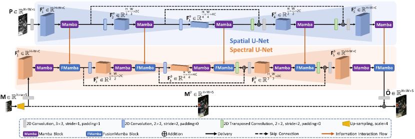
Figure 2. The overall architecture of our network. We incorporate Mamba blocks into two U-shape networks, namely the spatial U-Net and the spectral U-Net. The former extracts spatial features from $\mathbf{P}$, while the latter captures spectral characteristics from $\mathbf{M}$ and progressively achieves the fusion of $\mathbf{F}^{a}$ and $\mathbf{F}^{b}$.

2.3. Motivation

The existing DL-based methods for image fusion primarily apply CNNs or Transformers for feature extraction and information fusion. Although CNNs are efficient, they often struggle to capture global information. Conversely, Transformers exhibit outstanding global awareness but come with a notable computational cost. Fortunately, the recently proposed Mamba seems to offer a solution to this dilemma. However, directly stacking Mamba blocks for feature extraction is not advisable. Inspired by U2Net (Peng et al., 2023), we incorporate Mamba blocks into two distinct U-shape networks: the spatial U-Net and the spectral U-Net. This strategy enables the efficient learning of spatial and spectral characteristics separately and hierarchically. Apart from feature extraction, information integration is the most crucial part of image fusion tasks. Unfortunately, there have been few efforts to explore the potential of SSM in merging different types of information. Therefore, we expand the single-input Mamba block to support dual inputs, leading to the development of a novel module called the FusionMamba block, which can effectively integrate spatial and spectral information.

3. Method

3.1. Notations

The PAN/RGB image is denoted as $\mathbf{P}\in\mathbb{R}^{\rm{H\times W\times s}}$, where $\rm{H}$, $\rm{W}$, and $\rm{s}$ represent the height, width, and number of channels, respectively. $\mathbf{M}\in\mathbb{R}^{\rm{h\times w\times S}}$ denotes the LRMS/LRHS image, with $\rm{S}$ representing the number of spectral bands, $\rm{h=\frac{H}{4}}$, and $\rm{w=\frac{W}{4}}$. Besides, the up-sampled LRMS/LRHS image, the generated HRMS/HRHS image, and the ground-truth (GT) image are defined as ${\mathbf{M}}^{{U}}\in\mathbb{R}^{\rm{H\times W\times S}}$, $\mathbf{\tilde{O}}\in\mathbb{R}^{\rm{H\times W\times S}}$, and $\mathbf{O}\in\mathbb{R}^{\rm{H\times W\times S}}$, respectively. Furthermore, ${\mathbf{F}}^{{a}}_{{i}}$ and ${\mathbf{F}}^{b}_{i}$ represent spatial and spectral feature maps at the $i^{th}$ stage, with a total of five stages. The dimensions of ${\mathbf{F}}_{1}$ and ${\mathbf{F}}_{5}$ are $\rm{H\times W\times C}$, the dimensions of ${\mathbf{F}}_{2}$ and ${\mathbf{F}}_{4}$ are $\rm{\frac{H}{2}\times\frac{W}{2}\times 2C}$, and the dimensions of ${\mathbf{F}}_{3}$ are $\rm{\frac{H}{4}\times\frac{H}{4}\times 4C}$, where $\rm{C}$ denotes the number of channels. Additionally, $\rm{N}$ is the size of the hidden state in SSM.

3.2. Preliminaries

State Space Model. The SSM is a continuous system that maps a 1D input $x(t)\in\mathbb{R}$ into an output $y(t)\in\mathbb{R}$ through an intermediate hidden state $h(t)\in\mathbb{R}^{\rm{N}}$. Mathematically, it is often expressed using ordinary differential equations (ODEs), as illustrated below:

(1) $$h^{\prime}(t) =\mathbf{A}h(t)+\mathbf{B}x(t),$$

$$y(t) =\mathbf{C}h(t).$$

Here, $\mathbf{A}\in\mathbb{R}^{\rm{N\times N}}$ denotes the evolution parameter, while $\mathbf{B}\in\mathbb{R}^{\rm{N\times 1}}$ and $\mathbf{C}\in\mathbb{R}^{\rm{1\times N}}$ are the projection parameters. This equation suggests that SSM exhibits global awareness, as the current output is influenced by all preceding input data. When $\mathbf{A}$, $\mathbf{B}$, and $\mathbf{C}$ have constant values, Eq. 1 defines a linear time-invariant (LTI) system, which is the case in S4 (Gu et al., 2021a). Otherwise, it describes a linear time-varying (LTV) system, as in Mamba (Gu and Dao, 2023). LTI systems inherently lack the ability to perceive input content, whereas input-aware LTV systems are designed with this capability. This key distinction enables Mamba to surpass the limitations of SSM.

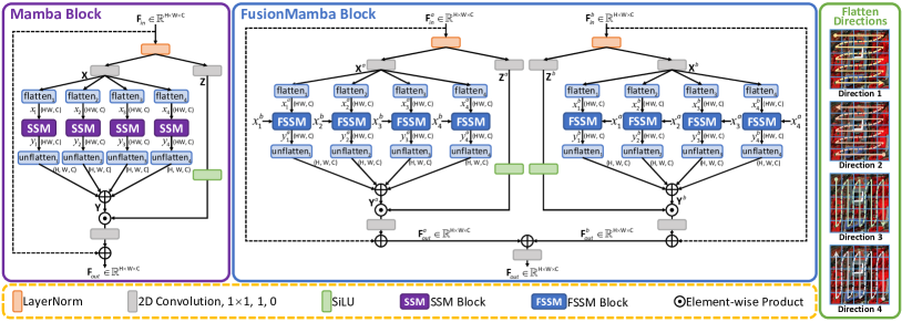
Figure 3. The schematic diagram of the Mamba block (left) and the proposed FusionMamba block (center), along with an illustration depicting the four flattening directions (right). The Mamba block is a single-input structure that extracts features, whereas the FusionMamba block is a dual-input structure specifically designed to integrate different types of information.

Discretization. When the SSM is employed in the field of DL, it necessitates discretization. To achieve this, a timescale parameter, denoted as $\mathbf{\Delta}\in\mathbb{R}$, is introduced to transform the continuous parameters $\mathbf{A}$ and $\mathbf{B}$ into discrete forms, represented as $\mathbf{\overline{A}}$ and $\mathbf{\overline{B}}$. By employing the zero-order hold (ZOH) as the transformation algorithm, the discrete parameters are expressed as follows:

(2) $$\mathbf{\overline{A}} =\rm{exp}(\mathbf{\Delta}\mathbf{A}),$$

$$\mathbf{\overline{B}} ={(\mathbf{\Delta}\mathbf{A})}^{-1}(\rm{exp}(\mathbf{\Delta}\mathbf{A})-{\mathbf{I}})\cdot\mathbf{\Delta}\mathbf{B}\approx\mathbf{\Delta}\mathbf{B}.$$

Then, the discrete form of Eq. 1 can be expressed as:

(3) $$h_{t} =\mathbf{\overline{A}}h_{t-1}+\mathbf{\overline{B}}x_{t},$$

$$y_{t} =\mathbf{C}h_{t}.$$

In practice, $x_{t}$ is a feature vector of size $\rm{C}$, and Eq. 3 operates independently on each of these features.

Selective Scan. In Mamba, since the parameters vary with the input, Eq. 3 cannot be reformulated in a convolutional form, which hinders the parallelization of SSM. To address this challenge, Mamba introduces the selective scan mechanism, which integrates three classical techniques: kernel fusion, parallel scan, and recomputation. Through the selective scan algorithm, Mamba achieves decent speed with a relatively low memory requirement.

[t] SSM Block [1] $x:\rm{{\color[rgb]{0,0.390625,0}(HW,C)}}$ $y:\rm{{\color[rgb]{0,0.390625,0}(HW,C)}}$ $\mathbf{A}:{\rm{{\color[rgb]{0,0.390625,0}(C,N)}}}\leftarrow\mathbf{Parameter}_{A}$ /* $\mathbf{A}$ represents ${\color[rgb]{0,0.390625,0}\rm{C}}$ sets of structured ${\color[rgb]{0,0.390625,0}\rm{N\times N}}$ matrices (Gu et al., 2021a) */ ${\mathbf{B}:{\rm{{\color[rgb]{0,0.390625,0}(HW,N)}}}\leftarrow\mathbf{Linear}_{B}}(x)$ ${\mathbf{C}:{\rm{{\color[rgb]{0,0.390625,0}(HW,N)}}}\leftarrow\mathbf{Linear}_{C}}(x)$ ${\mathbf{\Delta}:{\rm{{\color[rgb]{0,0.390625,0}(HW,C)}}}\leftarrow{\rm{log}}(1+{\rm{exp}}({\mathbf{Linear}_{\Delta}}}(x)+\mathbf{Parameter}_{\Delta}))$ /* $\mathbf{Parameter}_{\Delta}$ is a bias vector with a size of ${\color[rgb]{0,0.390625,0}\rm{C}}$ */ $\mathbf{\overline{A}}:{\rm{{\color[rgb]{0,0.390625,0}(HW,C,N)}}}\leftarrow\rm{exp(\mathbf{\Delta}\otimes\mathbf{A})}$ $\mathbf{\overline{B}}:\rm{{\color[rgb]{0,0.390625,0}(HW,C,N)}}\leftarrow\mathbf{\Delta}\otimes\mathbf{B}$ $y\leftarrow{\rm{SSM}(\mathbf{\overline{A}},\mathbf{\overline{B}},\mathbf{C})}(x)$ /* $\rm{SSM}$ represents Eq. 3 implemented by selective scan (Gu and Dao, 2023) */ $\mathbf{return}\;y$

3.3. Network Architecture

To fully exploit the potential of SSM, we incorporate Mamba blocks into a network structure inspired by (Peng et al., 2023), as depicted in Fig. 2. This architecture enables the independent and hierarchical learning of different types of information, primarily through two U-shape networks: the spatial U-Net and the spectral U-Net. The former extracts spatial details from $\mathbf{P}$, while the latter captures spectral characteristics from $\mathbf{M}$. To acquire sufficient deep-level information without excessively increasing the number of network parameters, we extract features at three different scales. This means that each U-Net comprises a total of five stages. At each stage, the feature map initially undergoes a Mamba block. Subsequently, it enters a FusionMamba block for information integration. Various types of convolution layers are then employed for up/down-sampling and adjusting the number of channels. Since $\mathbf{M}$ plays a more significant role in forming $\mathbf{\tilde{O}}$ compared to $\mathbf{P}$, FusionMamba blocks are specifically incorporated into the spectral U-Net to simulate the gradual injection of spatial information into spectral feature maps.

3.4. Mamba and FusionMamba Blocks

The schematic diagram of the Mamba and FusionMamba blocks within our network is illustrated in Fig. 3. To enhance spatial awareness, we adopt the four-directional sequence modeling method proposed in (Liu et al., 2024), which is shown on the right side of the diagram. This section provides detailed introductions for both the Mamba block and the proposed FusionMamba block, accompanied by an analysis of the required FLOPs.

[t] FSSM Block [1] $x^{a},x^{b}:\rm{{\color[rgb]{0,0.390625,0}(HW,C)}}$ $y^{a}:\rm{{\color[rgb]{0,0.390625,0}(HW,C)}}$ $\mathbf{A}:{\rm{{\color[rgb]{0,0.390625,0}(C,N)}}}\leftarrow\mathbf{Parameter}_{A}$ /* $\mathbf{A}$ represents ${\color[rgb]{0,0.390625,0}\rm{C}}$ sets of structured ${\color[rgb]{0,0.390625,0}\rm{N\times N}}$ matrices (Gu et al., 2021a) */ $\mathbf{B}:{\rm{{\color[rgb]{0,0.390625,0}(HW,N)}}}\leftarrow\mathbf{Linear}_{B}(x^{b})$ $\mathbf{C}:{\rm{{\color[rgb]{0,0.390625,0}(HW,N)}}}\leftarrow\mathbf{Linear}_{C}(x^{b})$ $\mathbf{\Delta}:{\rm{{\color[rgb]{0,0.390625,0}(HW,C)}}}\leftarrow{\rm{log}(1+{\rm{exp}}}(\mathbf{Linear}_{\Delta}(x^{b})+\mathbf{Parameter}_{\Delta}))$ /* $\mathbf{Parameter}_{\Delta}$ is a bias vector with a size of ${\color[rgb]{0,0.390625,0}\rm{C}}$ */ $\mathbf{\overline{A}}:{\rm{{\color[rgb]{0,0.390625,0}(HW,C,N)}}}\leftarrow\rm{exp(\mathbf{\Delta}\otimes\mathbf{A})}$ $\mathbf{\overline{B}}:\rm{{\color[rgb]{0,0.390625,0}(HW,C,N)}}\leftarrow\mathbf{\Delta}\otimes\mathbf{B}$ $y^{a}\leftarrow{\rm{SSM}(\mathbf{\overline{A}},\mathbf{\overline{B}},\mathbf{C})}(x^{a})$ /* $\rm{SSM}$ represents Eq. 3 implemented by selective scan (Gu and Dao, 2023) */ $\mathbf{return}\;y^{a}$

Mamba Block. For an input feature map $\mathbf{F}_{in}\in\mathbb{R}^{\rm{H\times W\times C}}$, we first normalize it using the widely employed layer normalization technique. Subsequently, it is processed by two parallel $1\times 1$ convolution layers, yielding two distinct feature maps, denoted as $\mathbf{X}\in\mathbb{R}^{\rm{H\times W\times C}}$ and $\mathbf{Z}\in\mathbb{R}^{\rm{H\times W\times C}}$. This process can be expressed as:

(4) $$\mathbf{X},\mathbf{Z}=\mathbf{Conv}_{{x}}(\mathbf{Norm}(\mathbf{F}_{in})),\mathbf{Conv}_{{z}}(\mathbf{Norm}(\mathbf{F}_{in})).$$

Here, $\mathbf{Norm}(\cdot)$ denotes layer normalization, while $\mathbf{Conv}_{x}(\cdot)$ and $\mathbf{Conv}_{z}(\cdot)$ represent the two convolution layers. After that, $\mathbf{X}$ is flattened in four directions, producing $x_{1}$, $x_{2}$, $x_{3}$, and $x_{4}$, each with dimensions of $\rm{HW\times C}$. These 1D sequences are then individually processed through SSM blocks for feature extraction, resulting in four outputs denoted as $y_{1}$, $y_{2}$, $y_{3}$, and $y_{4}$:

(5) $$\left\{\begin{array}[]{lr}{x_{i}}={\rm{flatten}}_{i}(\mathbf{X}),\\ {y_{i}}={\mathbf{SSM}}_{i}(x_{i}).\end{array}\right.i=1,2,3,4.$$

Here, ${\rm{flatten}}_{i}(\cdot)$ denotes the flattening operation along the $i^{th}$ direction, and ${\mathbf{SSM}}_{i}(\cdot)$ represents the $i^{th}$ SSM block. Alg. 3 provides a detailed explanation of the SSM block, where $\mathbf{Linear}(\cdot)$ defines the fully connected layer. Next, we unflatten the outputs of SSM blocks and combine them to obtain a new feature map, denoted as $\mathbf{Y}\in\mathbb{R}^{\rm{H\times W\times C}}$. This map is then gated by $\mathbf{Z}$. The resulting tensor undergoes a $1\times 1$ convolution layer and is added to $\mathbf{F}_{in}$, leading to the final output represented as $\mathbf{F}_{out}\in\mathbb{R}^{\rm{H\times W\times C}}$:

(6) $$\mathbf{Y} =\sum_{i}^{4}{\rm{unflatten}}_{i}(y_{i}),$$

$$\mathbf{F}_{out} ={\mathbf{Conv}}_{o}(\mathbf{Y}\cdot{\rm{SiLU}}(\mathbf{Z}))+\mathbf{F}_{in}.$$

Here, ${\rm{unflatten}}_{i}(\cdot)$ denotes the operation of unflattening along the $i^{th}$ direction. ${\mathbf{Conv}}_{o}(\cdot)$ represents the convolution layer, and ${\rm{SiLU}}(\cdot)$ defines the activate function ”SiLU”. For simplification, we express all the aforementioned processes as:

(7) $$\mathbf{F}_{out} =\mathbf{Mamba}(\mathbf{F}_{in}).$$

Here, $\mathbf{Mamba}(\cdot)$ denotes the Mamba block.

FusionMamba Block. The original SSM only supports a single input. To effectively integrate different types of information, we expand it to accommodate dual inputs, resulting in the Fusion State Space Model (FSSM), as detailed in Alg. 3.4. Within the FSSM block, one input is responsible for generating the projection and timescale parameters, while the other input is the sequence to be processed. Comprising eight FSSM blocks, the FusionMamba block is designed to be a symmetrical structure. For the input spatial and spectral feature maps, denoted as $\mathbf{F}_{in}^{a}\in\mathbb{R}^{\rm{H\times W\times C}}$ and $\mathbf{F}_{in}^{b}\in\mathbb{R}^{\rm{H\times W\times C}}$, we use the method in Mamba to generate two sets of feature maps:

(8) $$\mathbf{X}^{a},\mathbf{Z}^{a}=\mathbf{Conv}_{{x}}^{a}(\mathbf{Norm}(\mathbf{F}_{in}^{a})),\mathbf{Conv}_{{z}}^{a}(\mathbf{Norm}(\mathbf{F}_{in}^{a}));$$

$$\mathbf{X}^{b},\mathbf{Z}^{b}=\mathbf{Conv}_{{x}}^{b}(\mathbf{Norm}(\mathbf{F}_{in}^{b})),\mathbf{Conv}_{{z}}^{b}(\mathbf{Norm}(\mathbf{F}_{in}^{b})).$$

Since this equation is a direct extension of Eq. 4, explanations for the symbols are omitted. Next, $\mathbf{X}^{a}$ and $\mathbf{X}^{b}$ are flattened individually in four directions. The resulting 1D sequences are then forwarded to FSSM blocks for information integration:

(9) $$\left\{\begin{array}[]{lr}{x_{i}^{a}},{x_{i}^{b}}={\rm{flatten}}_{i}(\mathbf{X}^{a}),{\rm{flatten}}_{i}(\mathbf{X}^{b}),\\ {y_{i}^{a}},{y_{i}^{b}}={\mathbf{FSSM}}_{i}^{a}(x_{i}^{a},x_{i}^{b}),{\mathbf{FSSM}}_{i}^{b}(x_{i}^{b},x_{i}^{a}).\end{array}\right.i=1,2,3,4.$$

Here, $\mathbf{FSSM}^{a}(\cdot)$ and $\mathbf{FSSM}^{b}(\cdot)$ represent the FSSM blocks on the left and right halves of the FusionMamba block in Fig. 3. After that, we process the two sets of outputs separately, producing two new feature maps denoted as $\mathbf{Y}^{a}\in\mathbb{R}^{\rm{H\times W\times C}}$ and $\mathbf{Y}^{b}\in\mathbb{R}^{\rm{H\times W\times C}}$. These maps are subsequently combined to form $\mathbf{F}_{out}$:

(10) $$\mathbf{Y}^{a},\mathbf{Y}^{b} =\sum_{i}^{4}{\rm{unflatten}}_{i}(y_{i}^{a}),\sum_{i}^{4}{\rm{unflatten}}_{i}(y_{i}^{b}),$$

$$\mathbf{F}_{out}^{a} ={\mathbf{Conv}}_{o}^{a}(\mathbf{Y}^{a}\cdot{\rm{SiLU}}(\mathbf{Z}^{a}))+\mathbf{F}_{in}^{a},$$

$$\mathbf{F}_{out}^{b} ={\mathbf{Conv}}_{o}^{b}(\mathbf{Y}^{b}\cdot{\rm{SiLU}}(\mathbf{Z}^{b}))+\mathbf{F}_{in}^{b},$$

$$\mathbf{F}_{out} =\mathbf{Conv}_{o}(\mathbf{F}_{out}^{a}+\mathbf{F}_{out}^{b}).$$

Here, ${\mathbf{Conv}}_{o}^{a}(\cdot)$ and ${\mathbf{Conv}}_{o}^{b}(\cdot)$ denote the $1\times 1$ convolution layers that generate $\mathbf{F}_{out}^{a}$ and $\mathbf{F}_{out}^{b}$, respectively, while ${\mathbf{Conv}}_{o}(\cdot)$ represents the one that produces $\mathbf{F}_{out}$. To simplify, the aforementioned processes can be summarized as:

(11) $$\mathbf{F}_{out} =\mathbf{FMamba}(\mathbf{F}_{in}^{a},\mathbf{F}_{in}^{b}).$$

Here, $\mathbf{FMamba}(\cdot)$ denotes the FusionMamba block.

Analysis of FLOPs. For a convolution layer with $\rm{D}$ parameters, the FLOP count is typically calculated as $\rm{2HWD}$. In a Mamba block with the parameter number of $\rm{D}$, since a selective scan costs $\rm{9HWCN}$ FLOPs (Gu and Dao, 2023), the overall FLOP count is $\rm{2HWD+36HWCN}$. Furthermore, a FusionMamba block with the same number of parameters costs $\rm{2HWD+72HWCN}$ FLOPs. As for a self/cross-attention block in the Transformer, the overall FLOP count is estimated to be around $\rm{2HWD+4H^{2}W^{2}C}$. The FLOP comparison among these modules, as depicted in Fig. 4, indicates that the Mamba and FusionMamba blocks possess FLOP costs comparable to that of the convolution layer and are far more efficient than the self/cross-attention block. Notably, despite having the lowest FLOP requirement, the convolution layer lacks the ability to capture global information.

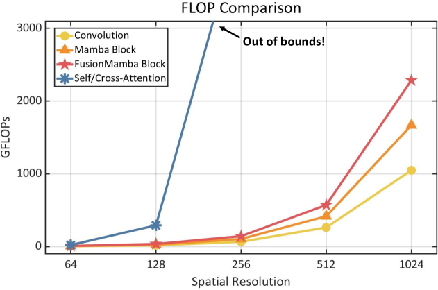
Figure 4. FLOP comparison among the four modules. For better visual effects, we set D, C, and N as 0.5M, 256, and 64.

3.5. Loss Function

The main contributions of this work lie in the application and innovation of SSM. Therefore, we utilize only the simplest $\ell_{1}$ loss function for network training, as shown below:

(12) $${\mathcal{L}oss}=\frac{1}{{\rm{T}}}\sum_{i}^{{\rm{T}}}{\|f_{\mathbf{\Theta}}({\mathbf{P}^{\{i\}},\mathbf{M}^{\{i\}}})-\mathbf{O}^{\{i\}}\|}_{1}.$$

Here, $\mathbf{P}^{\{i\}}$, $\mathbf{M}^{\{i\}}$, and $\mathbf{O}^{\{i\}}$ represent the $i^{th}$ PAN/RGB image, LRMS/LRHS image, and GT image in the training dataset. $f_{\mathbf{\Theta}}(\cdot)$ denotes our network with learnable parameters $\mathbf{\Theta}$, and ${\rm{T}}$ is the total number of training examples. Additionally, $\|\cdot\|_{1}$ defines the $\ell_{1}$ norm.

4. Experiments

4.1. Pansharpening

Table 1. Results on 20 reduced-resolution and 20 full-resolution samples of the WV3 dataset (Red: best; Blue: second best).

2*Method	2*Params	Reduced-Resolution				Full-Resolution (Real Data)
3-90.4pt		PSNR($\pm$std)	Q8($\pm$std)	SAM($\pm$std)	ERGAS($\pm$std)	${\rm{D}}_{\lambda}$($\pm$std)	${\rm{D}}_{s}$($\pm$std)	QNR($\pm$std)
GLP-FS (Vivone et al., 2018)18	$-$	32.963$\pm$2.753	0.833$\pm$0.092	5.315$\pm$1.765	4.700$\pm$1.597	0.0197$\pm$0.0078	0.0630$\pm$0.0289	0.9187$\pm$0.0347
BDSD-PC (Vivone, 2019)19	$-$	32.970$\pm$2.784	0.829$\pm$0.097	5.428$\pm$1.822	4.697$\pm$1.617	0.0625$\pm$0.0235	0.0730$\pm$0.0356	0.8698$\pm$0.0531
MSDCNN (Wei et al., 2017)17	0.23M	37.068$\pm$2.686	0.890$\pm$0.090	3.777$\pm$0.803	2.760$\pm$0.689	0.0230$\pm$0.0091	0.0467$\pm$0.0199	0.9316$\pm$0.0271
BDPN (Zhang et al., 2019)19	1.49M	36.191$\pm$2.702	0.871$\pm$0.100	4.201$\pm$0.857	3.046$\pm$0.732	0.0364$\pm$0.0142	0.0459$\pm$0.0192	0.9196$\pm$0.0308
FusionNet (Deng et al., 2021)21	0.08M	38.047$\pm$2.589	0.904$\pm$0.090	3.324$\pm$0.698	2.465$\pm$0.644	0.0239$\pm$0.0090	0.0364$\pm$0.0137	0.9406$\pm$0.0197
MUCNN (Wang et al., 2021)21	2.32M	38.262$\pm$2.703	0.911$\pm$0.089	3.206$\pm$0.681	2.400$\pm$0.617	0.0258$\pm$0.0111	0.0327$\pm$0.0140	0.9424$\pm$0.0205
LAGNet (Jin et al., 2022)22	0.15M	38.592$\pm$2.778	0.910$\pm$0.091	3.103$\pm$0.558	2.292$\pm$0.607	0.0368$\pm$0.0148	0.0418$\pm$0.0152	0.9230$\pm$0.0247
PMACNet (Liang et al., 2022)22	0.94M	38.595$\pm$2.882	0.912$\pm$0.092	3.073$\pm$0.623	2.293$\pm$0.532	0.0540$\pm$0.0232	0.0336$\pm$0.0115	0.9143$\pm$0.0281
U2Net (Peng et al., 2023)23	0.66M	39.117$\pm$3.009	0.920$\pm$0.085	2.888$\pm$0.581	2.149$\pm$0.525	0.0178$\pm$0.0072	0.0313$\pm$0.0075	0.9514$\pm$0.0115
Pan-Mamba (He et al., 2024)24	0.48M	39.012$\pm$2.818	0.920$\pm$0.085	2.914$\pm$0.592	2.184$\pm$0.521	0.0183$\pm$0.0071	0.0307$\pm$0.0108	0.9516$\pm$0.0146
FusionMamba	0.77M	39.283$\pm$2.986	0.921$\pm$0.085	2.848$\pm$0.571	2.107$\pm$0.507	0.0175$\pm$0.0069	0.0294$\pm$0.0043	0.9536$\pm$0.0093
Ideal value	$-$	+$\infty$	1	0	0	0	0	1

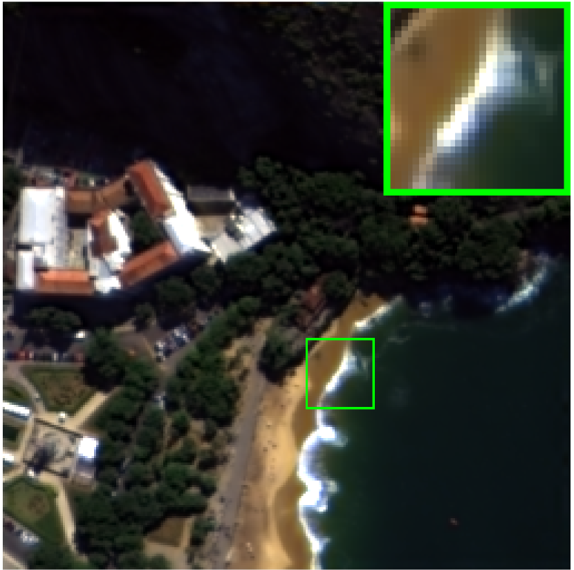
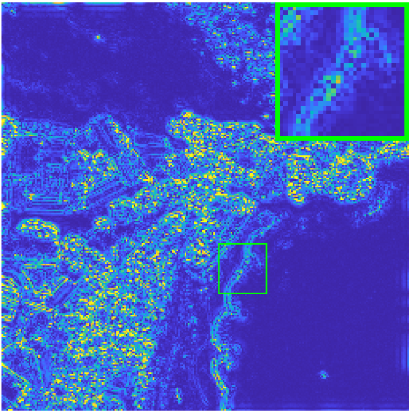
GLP-FS

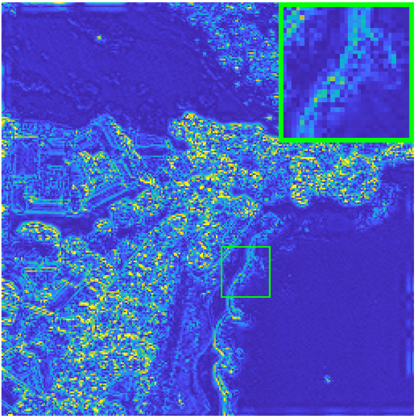
BDSD-PC

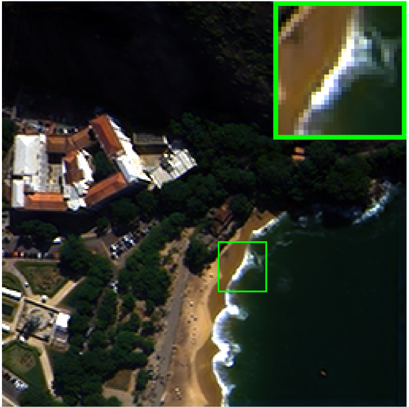
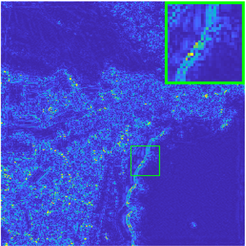
MSDCNN

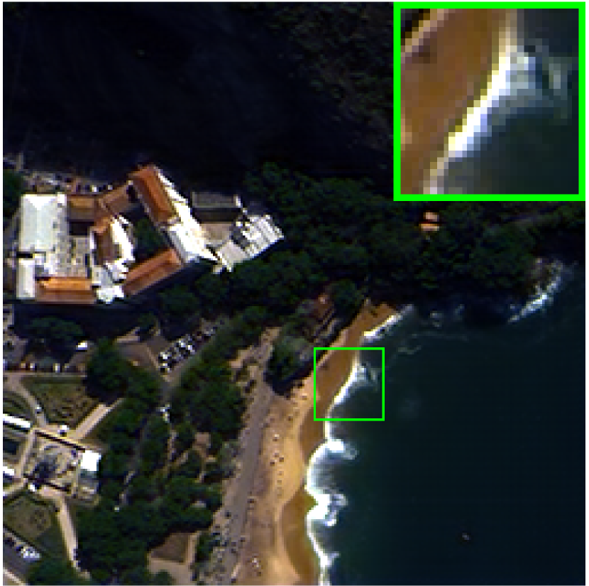
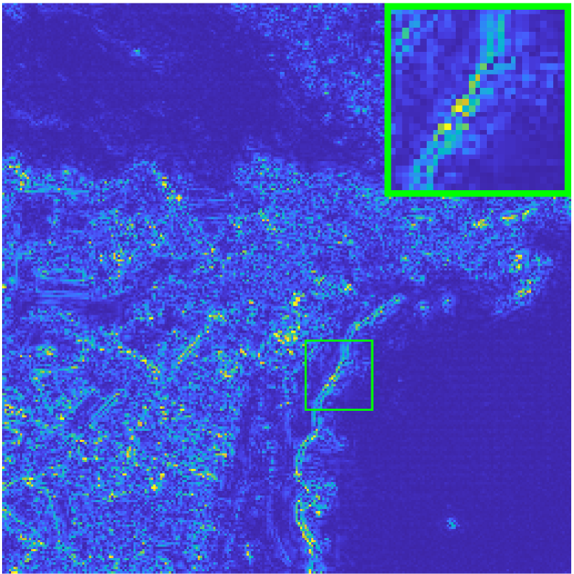
BDPN

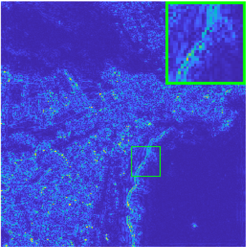
FusionNet

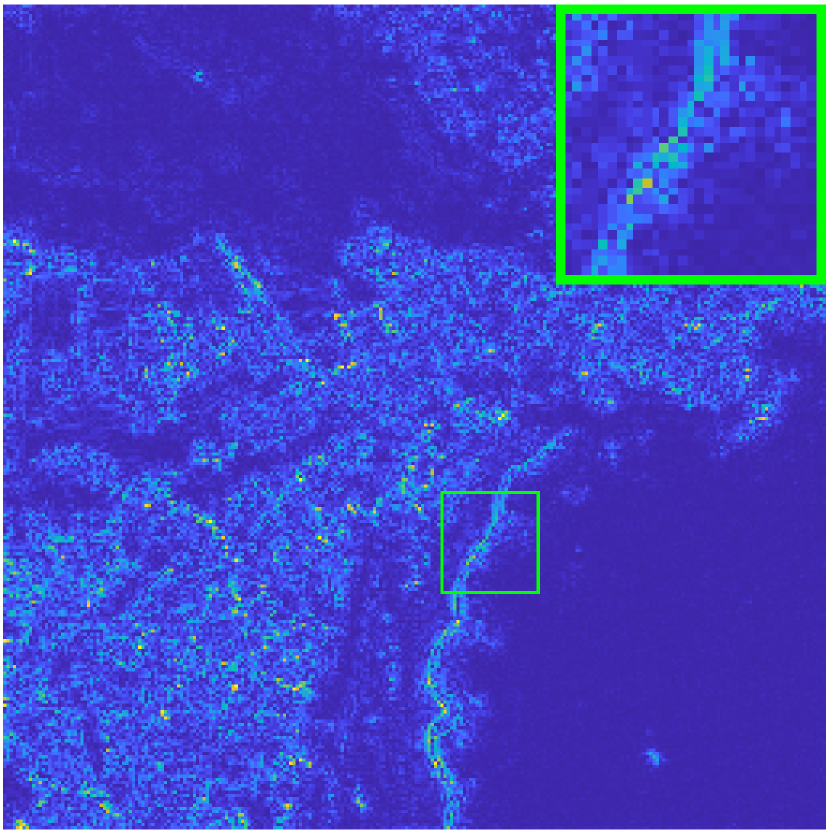
MUCNN

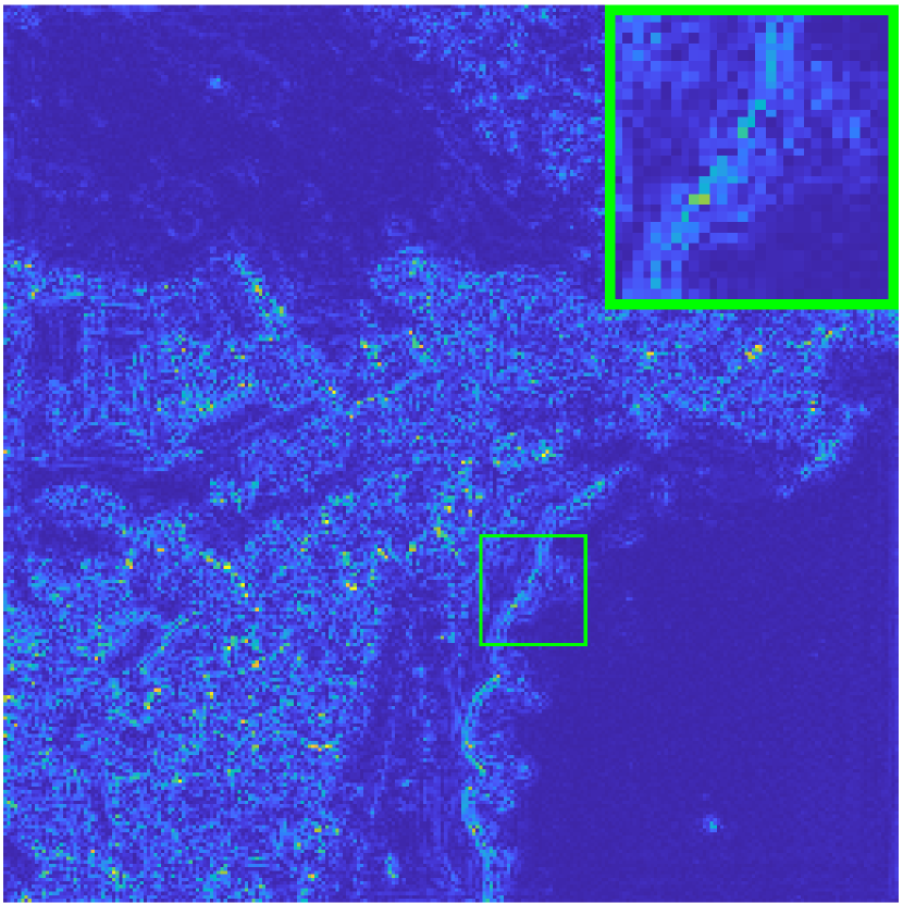
LAGNet

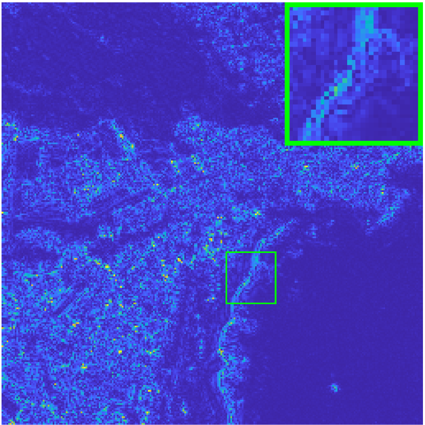
PMACNet

U2Net

Pan-Mamba

FusionMamba

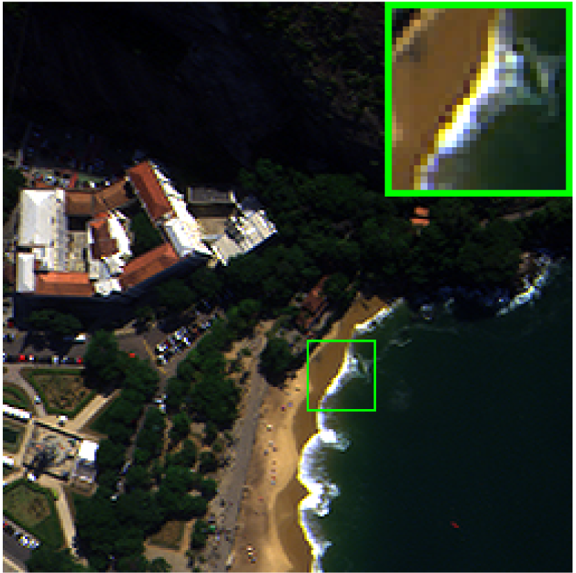
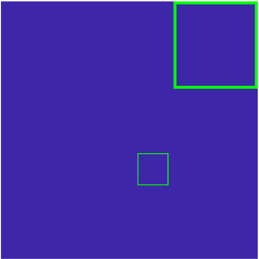
GT

Figure 5. Qualitative evaluation results on a reduced-resolution example of the WV3 dataset. Rows 1: Natural color maps for spectral bands 1, 3, and 5. Rows 2: The corresponding absolute error maps (AEMs) for the spectral band 7.

Dataset. For the pansharpening task, we conduct experiments on the WorldView-3 (WV3) dataset. This dataset consists of $10,000$ training samples, with 90% allocated for training and 10% for validation. Furthermore, it contains 20 reduced-resolution and 20 full-resolution testing samples. Each training sample comprises an image triplet in the PAN/LRMS/GT format, with dimensions of $64\times 64\times 1$, $16\times 16\times 8$, and $64\times 64\times 8$, respectively. The reduced-resolution testing samples are composed of PAN/LRMS/GT image triplets sized $256\times 256\times 1$, $64\times 64\times 8$, and $256\times 256\times 8$. Additionally, the full-resolution testing samples consist of PAN/LRMS image pairs of sizes $512\times 512\times 1$ and $128\times 128\times 8$. The dataset utilized in this section is sourced from the PanCollection proposed in (Deng et al., 2022). For further details, please refer to the Sup. Mat.

Benchmarks and Evaluation Metrics. We compare the proposed method with recent SOTA works, including two traditional approaches: GLP-FS (Vivone et al., 2018) and BDSD-PC (Vivone, 2019); and eight DL-based methods: MSDCNN (Wei et al., 2017), BDPN (Zhang et al., 2019), FusionNet (Deng et al., 2021), MUCNN (Wang et al., 2021), LAGNet (Jin et al., 2022), PMACNet (Liang et al., 2022), U2Net (Peng et al., 2023), and Pan-Mamba (He et al., 2024). To ensure fairness, all DL-based methods are trained using the same Nvidia GPU-3090 and PyTorch environment. In accordance with the research standard of pansharpening, we employ four metrics: PSNR (Wang et al., 2004), Q8 (Garzelli and Nencini, 2009), SAM, and ERGAS (Wald et al., 1997), to assess the quality of results on the reduced-resolution samples. For the full-resolution samples, we choose ${\rm{D}}_{\lambda}$, ${\rm{D}}_{s}$, and QNR (Vivone et al., 2015) as the quality indicators.

Network and Training Settings. In the pansharpening task, we set $\rm{C}$ and $\rm{N}$ to 32 and 8. For training, the epoch, batch size, and initial learning rate are configured as 400, 32, and $5\times 10^{-4}$, respectively. Additionally, we utilize the Adam optimizer and halve the learning rate every 200 epochs. As for other DL-based methods, we adhere to the default settings outlined in the related papers or codes. For more information, please consult the Sup. Mat.

Evaluation Results. The quantitative evaluation outcomes are shown in Tab. 1, where FusionMamba yields the best average results across all metrics. Considering that the indicator values are already approaching their limits, our method has achieved notable improvements compared to alternative techniques. In addition, the qualitative evaluation results are depicted in Fig. 5, with FusionMamba possessing the darkest absolute error map (AEM). Thus, it is clear that our method surpasses other SOTA approaches.

Table 2. Quantitative evaluation results on testing samples of the Pavia, Botswana, and WDC datasets.

2*Method	2*Params	Pavia					Botswana					WDC
3-170.4pt		PSNR	CC	SSIM	SAM	ERGAS	PSNR	CC	SSIM	SAM	ERGAS	PSNR	CC	SSIM	SAM	ERGAS
GLP (Aiazzi et al., 2006)06	$-$	31.944	0.935	0.749	6.099	4.909	32.559	0.951	0.837	1.383	1.207	27.946	0.934	0.761	6.546	5.110
Hysure (Simões et al., 2015)15	$-$	32.208	0.921	0.730	6.240	5.474	30.610	0.928	0.796	1.747	1.595	25.598	0.913	0.718	7.254	5.834
HyperPNN (He et al., 2019b)19	0.13-0.14M	33.394	0.963	0.827	4.566	3.750	33.114	0.961	0.873	1.366	1.195	29.258	0.945	0.860	4.051	5.749
HSpeNet1 (He et al., 2020)20	0.18-0.19M	33.612	0.964	0.824	4.690	3.721	31.746	0.942	0.844	1.456	1.663	29.634	0.960	0.870	4.039	4.266
HSpeNet2 (He et al., 2020)20	0.11-0.13M	33.472	0.962	0.819	4.642	3.818	32.575	0.953	0.849	1.400	1.348	29.700	0.961	0.872	4.009	4.261
FusionNet (Deng et al., 2021)21	0.21-0.26M	34.739	0.969	0.847	4.462	3.446	32.506	0.952	0.850	1.397	1.367	29.696	0.959	0.866	3.917	4.339
Hyper-DSNet (Zhuo et al., 2022)22	0.18-0.31M	34.376	0.969	0.849	4.295	3.434	33.538	0.964	0.876	1.305	1.126	30.232	0.964	0.875	4.102	3.943
FPFNet (Dong et al., 2023)23	3.00-3.06M	33.581	0.959	0.825	4.627	3.931	33.451	0.962	0.871	1.369	1.135	30.291	0.957	0.855	4.440	4.250
FusionMamba	0.58-0.59M	35.610	0.973	0.871	3.979	3.164	33.945	0.966	0.880	1.278	1.079	31.003	0.965	0.881	3.772	3.793
Ideal value	$-$	+$\infty$	1	1	0	0	+$\infty$	1	1	0	0	+$\infty$	1	1	0	0

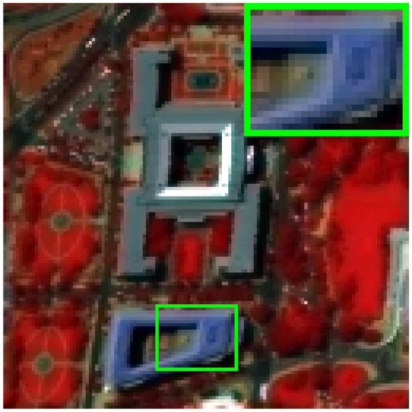
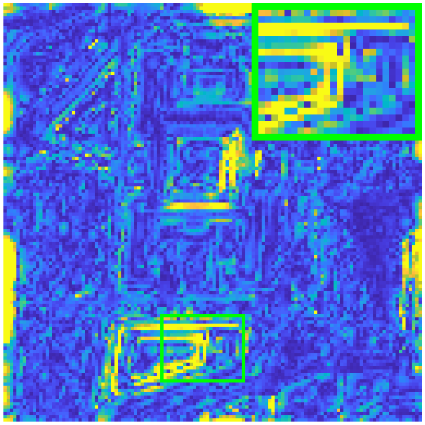
GLP

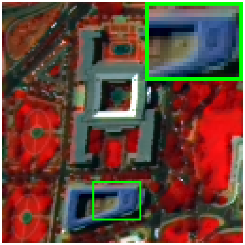
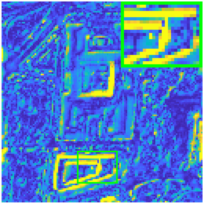
HySure

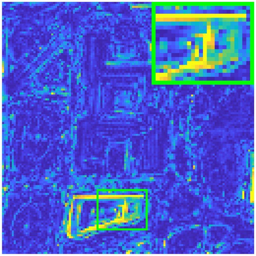
HyperPNN

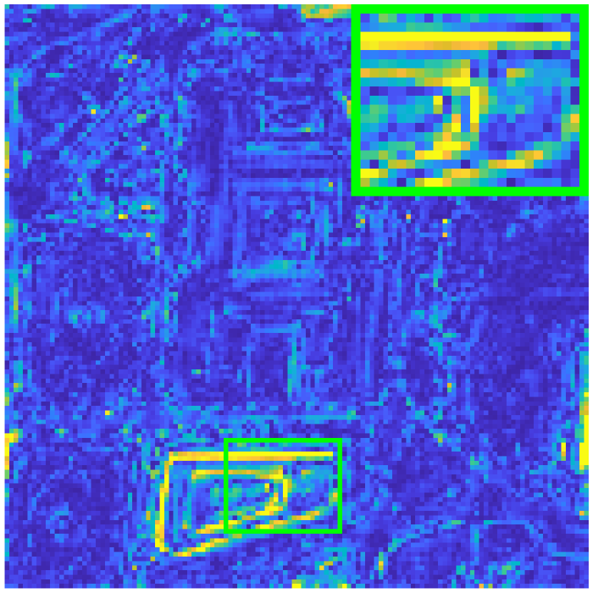
HSpeNet1

HSpeNet2

FusionNet

Hyper-DSNet

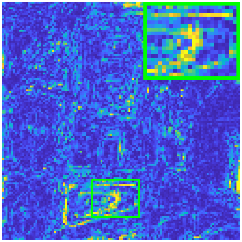
FPFNet

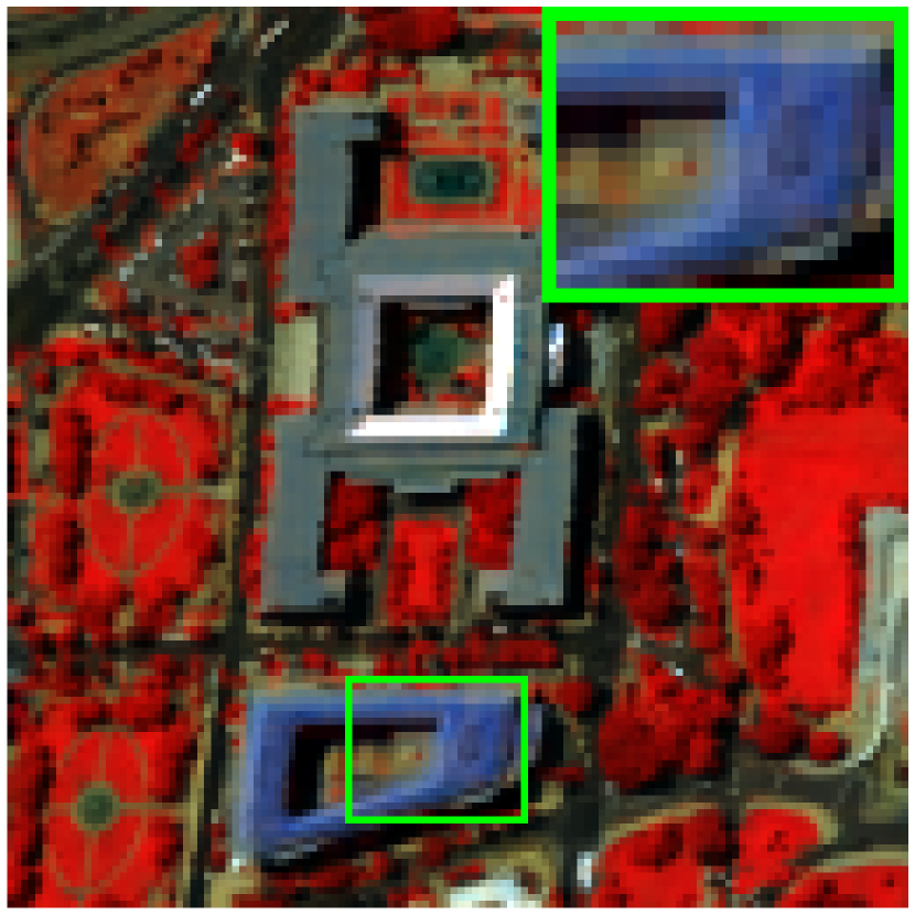
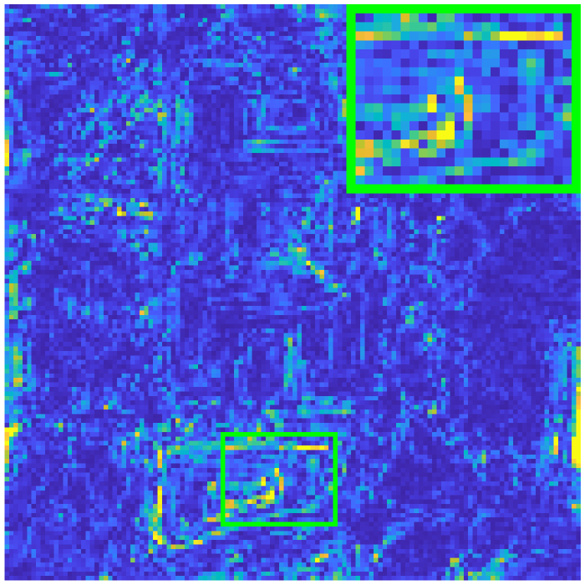
FusionMamba

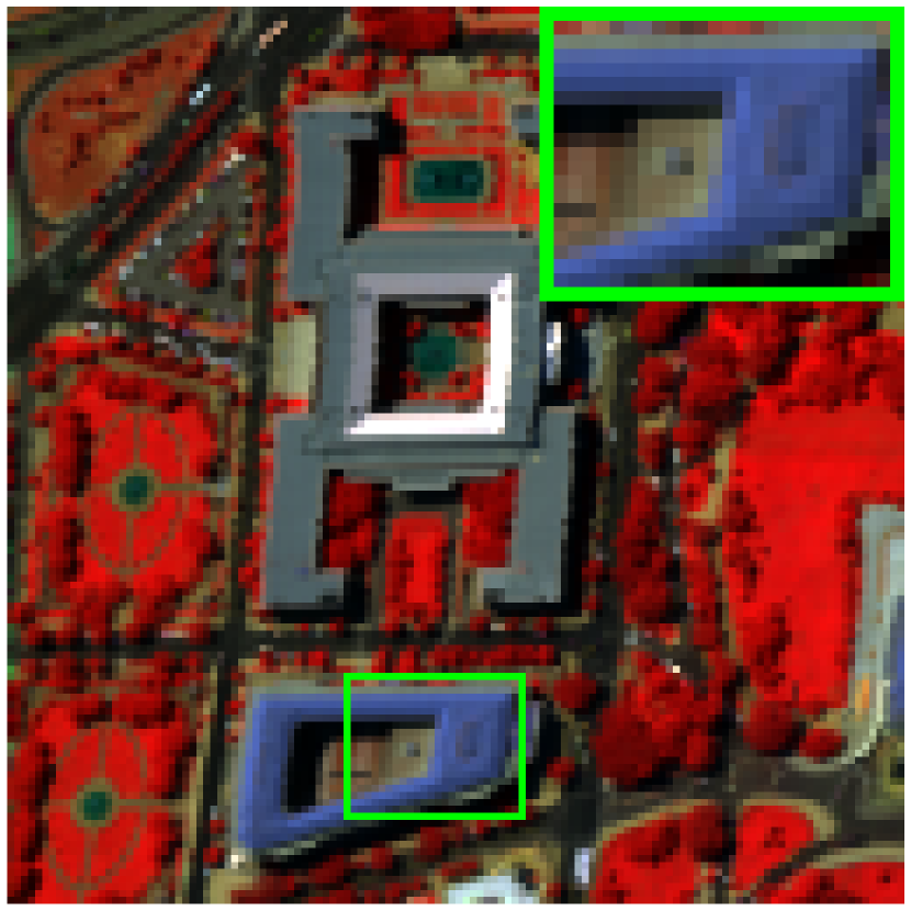
GT

Figure 6. Qualitative evaluation results on the WDC dataset. Row 1: Natural color maps for spectral bands 20, 50, and 80. Row 2: The corresponding AEMs for the spectral band 25.

4.2. Hyper-Spectral Pansharpening

Datasets. For the hyper-spectral pansharpening task, we perform experiments on three popular datasets: Pavia, Botswana, and Washington DC (WDC). The Pavia dataset contains 1680 training samples, with 90% designated for training and 10% for validation. Additionally, this dataset includes 2 testing samples. Each training sample consists of an image triplet in the PAN/LRHS/GT format, with sizes of $64\times 64\times 1$, $16\times 16\times 102$, and $64\times 64\times 102$, respectively. The testing samples are PAN/LRHS/GT image triplets sized $400\times 400\times 1$, $100\times 100\times 102$, and $400\times 400\times 102$. The Botswana dataset comprises 967 training samples, with 83% allocated for training and 17% for validation, in addition to 4 testing samples. Each training sample encompasses a PAN/LRHS/GT image triplet with dimensions of $64\times 64\times 1$, $16\times 16\times 145$, and $64\times 64\times 145$, respectively. The testing samples are PAN/LRHS/GT image triplets of sizes $128\times 128\times 1$, $32\times 32\times 145$, and $128\times 128\times 145$. In the WDC dataset, there are 1024 training samples, divided into 90% for training and 10% for validation, with an additional 4 samples for testing. Each training sample contains a PAN/LRHS/GT image triplet of sizes $64\times 64\times 1$, $16\times 16\times 191$, and $64\times 64\times 191$. The testing samples consist of PAN/LRHS/GT image triplets sized $128\times 128\times 1$, $32\times 32\times 191$, and $128\times 128\times 191$. All datasets employed in this section are sourced from the HyperPanCollection presented in (Zhuo et al., 2022).

Benchmarks and Evaluation Metrics. The proposed method is compared against several SOTA works, including two traditional approaches: GLP (Aiazzi et al., 2006) and Hysure (Simões et al., 2015); and five DL-based methods: HyperPNN (He et al., 2019b), HSpeNet series (He et al., 2020), FusionNet (Deng et al., 2021), Hyper-DSNet (Zhuo et al., 2022), and FPFNet (Dong et al., 2023). We select five widely used metrics for evaluation, namely PSNR, Cross-Correlation (CC), SSIM (Wang et al., 2004), and ERGAS.

Network and Training Settings. For hyper-spectral pansharpening, we set $\rm{C}$ to 48 and $\rm{N}$ to 8. Furthermore, in U-shaped networks, the channel number of the feature maps remains unchanged, a slight deviation from the depiction in Fig. 3. During the training of our network on the Pavia/Botswana/WDC datasets, we configure the epoch, batch size, and initial learning rate as 2000/2500/2000, 32/32/32, and 2/2/2$\times 10^{-4}$. Besides, we choose Adam as the optimizer, with the learning rate decreasing by half every 1000 epochs.

Evaluation Results. The quantitative and qualitative assessment results are presented in Tab. 2 and Fig. 6, respectively. Clearly, FusionMamba outperforms other approaches by a significant margin.

Table 3. Quantitative evaluation results on the CAVE dataset.

Method	Params	PSNR	SSIM	SAM	ERGAS
LTMR(Dian and Li, 2019)19	$-$	36.54$\pm$3.30	0.963$\pm$0.021	6.71$\pm$2.19	5.39$\pm$2.53
UTV(Xu et al., 2020)20	$-$	38.60$\pm$4.06	0.941$\pm$0.043	8.65$\pm$3.38	4.52$\pm$2.82
IR-TenSR(Xu et al., 2022)22	$-$	35.61$\pm$3.45	0.945$\pm$0.027	12.3$\pm$4.68	5.90$\pm$3.05
ResTFNet(Liu et al., 2018)18	2.39M	45.58$\pm$5.47	0.994$\pm$0.006	2.76$\pm$0.70	2.31$\pm$2.44
SSRNet(Zhang et al., 2021)21	0.03M	48.62$\pm$3.92	0.995$\pm$0.002	2.54$\pm$0.84	1.64$\pm$1.22
Fusformer(Hu et al., 2022)22	0.50M	49.98$\pm$8.10	0.994$\pm$0.011	2.20$\pm$0.85	2.53$\pm$5.31
3DT-Net(Ma et al., 2023)23	3.16M	51.47$\pm$4.05	0.997$\pm$0.002	2.12$\pm$0.70	1.12$\pm$0.94
PSRT(Deng et al., 2023)23	0.25M	50.59$\pm$5.99	0.996$\pm$0.003	2.15$\pm$0.64	3.55$\pm$0.99
U2Net(Peng et al., 2023)23	2.65M	50.44$\pm$4.12	0.997$\pm$0.002	2.19$\pm$0.64	1.26$\pm$0.90
FusionMamba	2.56M	51.62$\pm$4.00	0.998$\pm$0.002	2.02$\pm$0.61	1.10$\pm$0.81
Ideal value	$-$	+$\infty$	1	0	0

LTMR

UTV

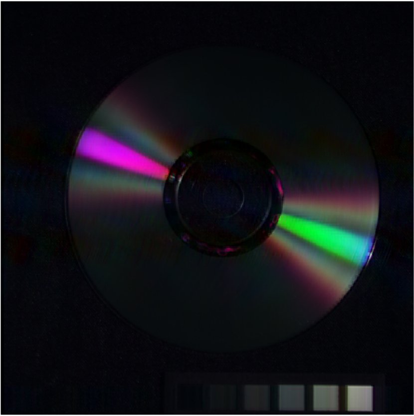
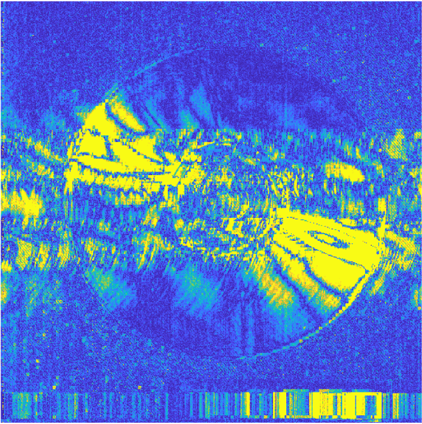
IR-TenSR

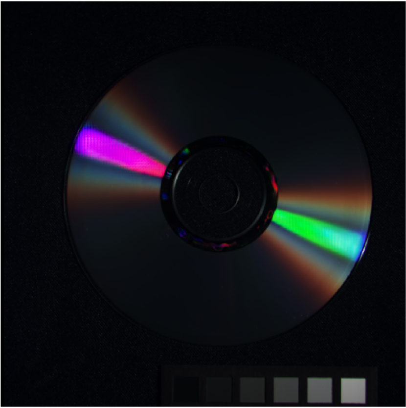
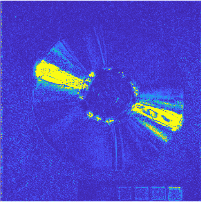
ResTFNet

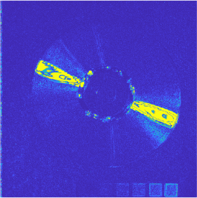
SSRNet

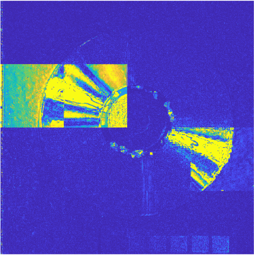
Fusformer

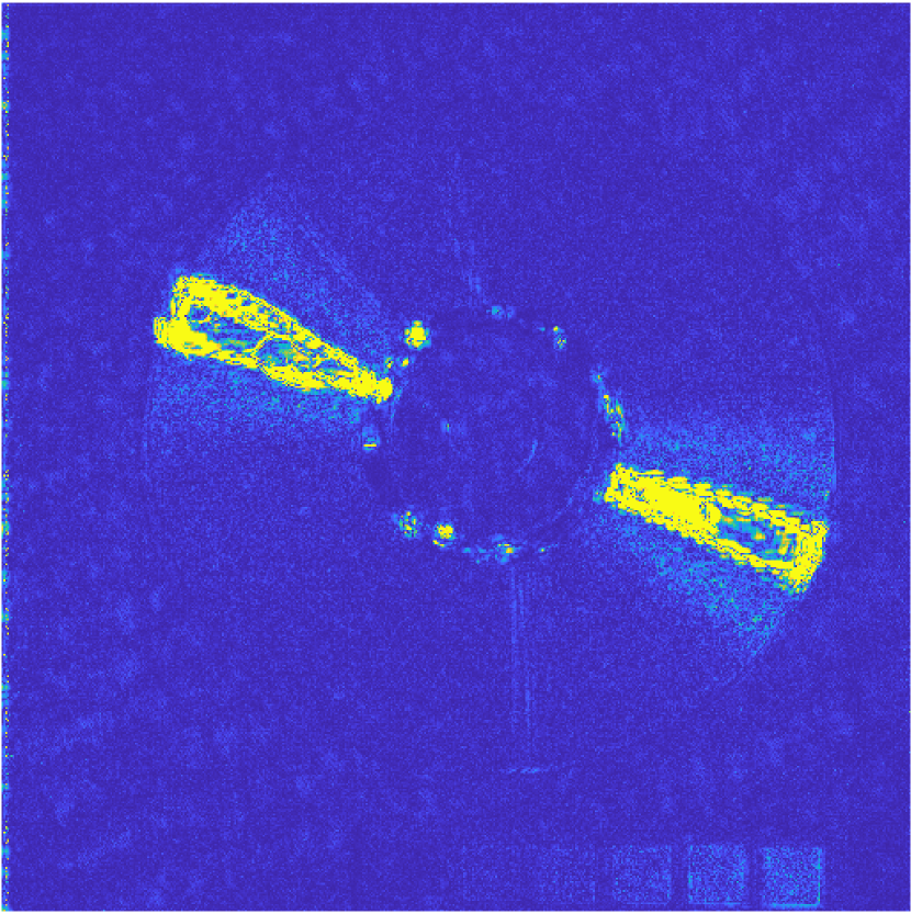
3DT-Net

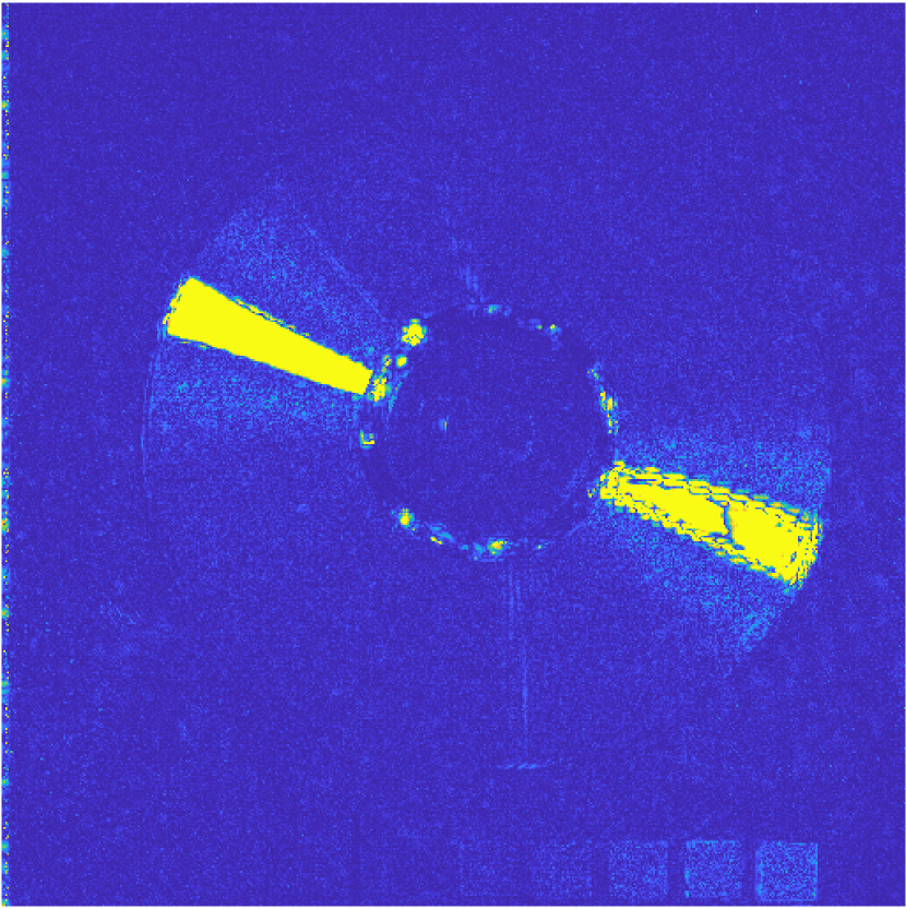
PSRT

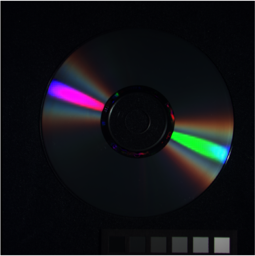
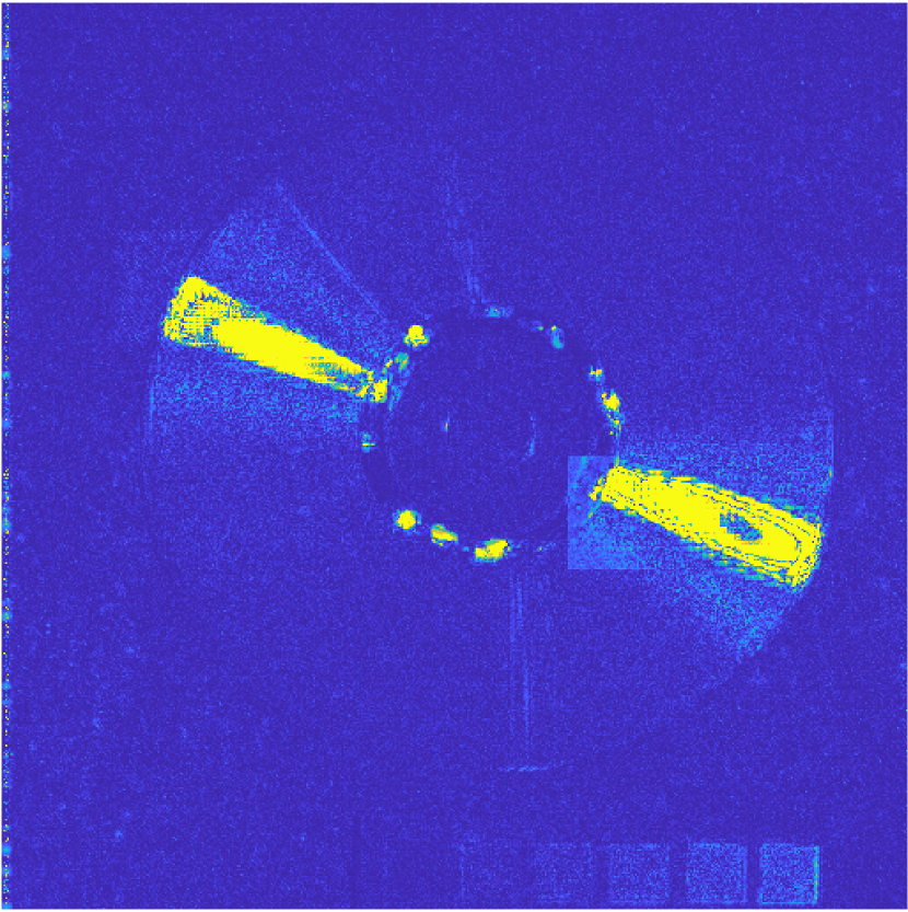
U2Net

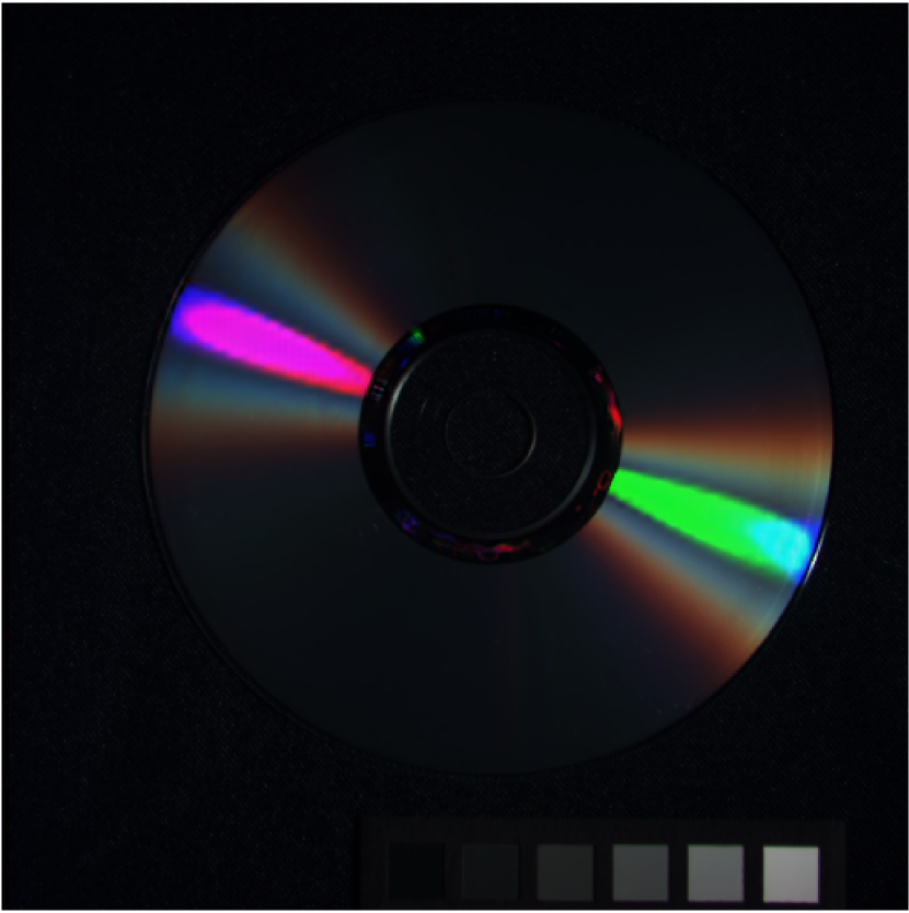
FusionMamba

GT

Figure 7. Results on the CAVE dataset. Row 1: Natural color maps for bands 6, 13, and 26. Row 2: AEMs for band 13.

4.3. HISR

Dataset. For the HISR task, we perform experiments on the well-known CAVE dataset (Yasuma et al., 2010), which consists of 32 RGB/LRHS image pairs. We select 20 pairs for training purposes and reserve the remaining pairs for testing. The training data is cropped into 3920 overlapped RGB/LRHS/RGB image triplets (80% allocated for training and 20% for validation) of dimensions $64\times 64\times 3$, $16\times 16\times 31$, and $64\times 64\times 31$, respectively. In addition, the testing data is processed to form 12 RGB/LRHS/GT image triplets, sized $512\times 512\times 3$, $128\times 128\times 31$, and $512\times 512\times 31$.

Benchmarks and Evaluation Metrics. We compare FusionMamba with recent SOTA works for HISR, including three traditional algorithms: LTMR (Dian and Li, 2019), UTV (Xu et al., 2020), and IR-TenSR (Xu et al., 2022); and six DL-based methods: ResTFNet (Liu et al., 2018), SSRNet (Zhang et al., 2021), Fusformer (Hu et al., 2022), 3DT-Net (Ma et al., 2023), PSRT (Deng et al., 2023), and U2Net (Peng et al., 2023). We choose four widely employed metrics for evaluation: PSNR, SSIM, SAM, and ERGAS.

Network and Training Settings. In the HISR task, we set $\rm{C}$ and $\rm{N}$ to 64 and 4. During training, we configure the epoch, batch size, and initial learning rate as 1100, 32, and $2\times 10^{-4}$, respectively. Additionally, Adam is employed as the optimizer, and the learning rate undergoes halving every 500 epochs.

Evaluation Results. The quantitative and qualitative assessment results are presented in Tab. 3 and Fig. 7, respectively. Our method demonstrates superior performance compared to other approaches.

4.4. Ablation Study

Table 4. Ablation study on network design.

Method	Description	PSNR	Q8	SAM	ERGAS
V1	without U-Nets	39.003	0.918	2.920	2.181
V2	a single U-Net	39.077	0.918	2.893	2.159
V3	one-directional scan	39.086	0.919	2.903	2.158
V4	bidirectional scan	39.125	0.918	2.895	2.151
V5	$\mathbf{F}^{a}_{out}$ as the output	38.872	0.918	2.920	2.217
V6	$\mathbf{F}^{b}_{out}$ as the output	38.849	0.918	2.935	2.230
Ours	$-$	39.283	0.921	2.848	2.107

Effectiveness of Network Design. To validate the effectiveness of our network design, we devise six variants of the proposed FusionMamba. The first variant (V1) does not employ U-shape networks for feature extraction, while the second variant (V2) combines the spatial and spectral U-Nets into a single U-Net. V1 and V2 are designed to showcase the effectiveness of our dual U-shape network architecture. Additionally, the third and fourth variants (V3 & V4) replace the four-directional sequence modeling in the Mamba and FusionMamba blocks with single-directional and bidirectional scans (Zhu et al., 2024), respectively. These modifications enable us to evaluate the impact of different flattening approaches on performance. Furthermore, the fifth variant (V5) directly considers $\mathbf{F}^{a}_{out}$ as the output of the FusionMamba block, whereas the sixth variant (v6) utilizes $\mathbf{F}^{b}_{out}$ as its output. These variants are created to assess the effectiveness of our FusionMamba block design. We evaluate these methods on the reduced-resolution samples of the WV3 dataset. For a fair comparison, we ensure that all networks have an equal number of parameters. The results, as presented in Fig. 4, clearly demonstrate the effectiveness of our network design.

Table 5. Ablation study on Mamba and FusionMamba blocks.

Method	GFLOPs	PSNR	Q8	SAM	ERGAS
Conv+Concat	12.1	38.750	0.917	2.995	2.249
Mamba+Concat	20.9	38.769	0.917	2.942	2.249
Conv+FMamba	21.6	39.114	0.920	2.888	2.153
SA+CA	5000	38.933	0.918	2.956	2.198
Mamba+CA	2500	39.129	0.919	2.894	2.150
SA+FMamba	2500	39.157	0.920	2.872	2.141
Ours	30.4	39.283	0.921	2.848	2.107

Effectiveness of Mamba and FusionMamba Blocks. To validate the efficacy of the Mamba block in feature extraction, we substitute it with the convolution layer (Conv) and self-attention module (SA). In terms of the FusionMamba block (FMamba) for information fusion, we replace it with the concatenation operation (Concat) and cross-attention module (CA). These changes result in six different variants of the proposed method. We assess the performance of these variants using the reduced-resolution samples from the WV3 dataset and ensure that all networks have the same number of parameters. The quantitative evaluation results, as shown in Fig. 5, clearly demonstrate that the proposed method achieves the best performance with a reasonable number of FLOPs.

5. Conclusion

In this paper, we introduce FusionMamba, a novel method for efficient image fusion. To effectively extract different features, we incorporate Mamba blocks into two U-shaped networks: the spatial U-Net and the spectral U-Net. This approach enables the efficient learning of spatial and spectral characteristics separately and hierarchically. Furthermore, to achieve comprehensive information fusion, we expand the Mamba block to accommodate dual inputs, resulting in a new module called the FusionMamba block. The FusionMamba achieves SOTA performance on five datasets across three image fusion tasks, highlighting the effectiveness of our method.

References

- (1)
- Aiazzi et al. (2006) Bruno Aiazzi, L Alparone, Stefano Baronti, Andrea Garzelli, and Massimo Selva. 2006. MTF-tailored multiscale fusion of high-resolution MS and Pan imagery. Photogrammetric Engineering & Remote Sensing 72, 5 (2006), 591–596.
- Chen et al. (2024) Tianxiang Chen, Zhentao Tan, Tao Gong, Qi Chu, Yue Wu, Bin Liu, Jieping Ye, and Nenghai Yu. 2024. MiM-ISTD: Mamba-in-Mamba for Efficient Infrared Small Target Detection. arXiv preprint arXiv:2403.02148 (2024).
- Deng et al. (2021) Liang-Jian Deng, Gemine Vivone, Cheng Jin, and Jocelyn Chanussot. 2021. Detail Injection-Based Deep Convolutional Neural Networks for Pansharpening. IEEE Transactions on Geoscience and Remote Sensing 59, 8 (2021), 6995–7010. https://doi.org/10.1109/TGRS.2020.3031366
- Deng et al. (2022) Liang-jian Deng, Gemine Vivone, Mercedes E. Paoletti, Giuseppe Scarpa, Jiang He, Yongjun Zhang, Jocelyn Chanussot, and Antonio Plaza. 2022. Machine Learning in Pansharpening: A benchmark, from shallow to deep networks. IEEE Geoscience and Remote Sensing Magazine 10, 3 (2022), 279–315. https://doi.org/10.1109/MGRS.2022.3187652
- Deng et al. (2023) Shang-Qi Deng, Liang-Jian Deng, Xiao Wu, Ran Ran, Danfeng Hong, and Gemine Vivone. 2023. PSRT: Pyramid shuffle-and-reshuffle transformer for multispectral and hyperspectral image fusion. IEEE Transactions on Geoscience and Remote Sensing 61 (2023), 1–15.
- Dian and Li (2019) Renwei Dian and Shutao Li. 2019. Hyperspectral image super-resolution via subspace-based low tensor multi-rank regularization. IEEE Transactions on Image Processing 28, 10 (2019), 5135–5146.
- Dong et al. (2023) Wenqian Dong, Yihan Yang, Jiahui Qu, Yunsong Li, Yufei Yang, and Xiuping Jia. 2023. Feature Pyramid Fusion Network for Hyperspectral Pansharpening. IEEE Transactions on Neural Networks and Learning Systems (2023), 1–13. https://doi.org/10.1109/TNNLS.2023.3325887
- Fu et al. (2022) Daniel Y Fu, Tri Dao, Khaled K Saab, Armin W Thomas, Atri Rudra, and Christopher Ré. 2022. Hungry hungry hippos: Towards language modeling with state space models. arXiv preprint arXiv:2212.14052 (2022).
- Garzelli and Nencini (2009) Andrea Garzelli and Filippo Nencini. 2009. Hypercomplex Quality Assessment of Multi/Hyperspectral Images. IEEE Geoscience and Remote Sensing Letters 6, 4 (2009), 662–665. https://doi.org/10.1109/LGRS.2009.2022650
- Giuseppe et al. (2016) Masi Giuseppe, Cozzolino Davide, Verdoliva Luisa, and Scarpa Giuseppe. 2016. Pansharpening by Convolutional Neural Networks. Remote Sensing 8, 7 (2016), 594.
- Gu and Dao (2023) Albert Gu and Tri Dao. 2023. Mamba: Linear-time sequence modeling with selective state spaces. arXiv preprint arXiv:2312.00752 (2023).
- Gu et al. (2021a) Albert Gu, Karan Goel, and Christopher Ré. 2021a. Efficiently modeling long sequences with structured state spaces. arXiv preprint arXiv:2111.00396 (2021).
- Gu et al. (2021b) Albert Gu, Isys Johnson, Karan Goel, Khaled Saab, Tri Dao, Atri Rudra, and Christopher Ré. 2021b. Combining recurrent, convolutional, and continuous-time models with linear state space layers. Advances in neural information processing systems 34 (2021), 572–585.
- Gu et al. (2018) Jiuxiang Gu, Zhenhua Wang, Jason Kuen, Lianyang Ma, Amir Shahroudy, Bing Shuai, Ting Liu, Xingxing Wang, Gang Wang, Jianfei Cai, et al. 2018. Recent advances in convolutional neural networks. Pattern recognition 77 (2018), 354–377.
- He et al. (2016) Kaiming He, Xiangyu Zhang, Shaoqing Ren, and Jian Sun. 2016. Deep residual learning for image recognition. In Proceedings of the IEEE Conference on Computer Vision and Pattern Recognition (CVPR). 770–778.
- He et al. (2019a) Lin He, Yizhou Rao, Jun Li, Jocelyn Chanussot, Antonio Plaza, Jiawei Zhu, and Bo Li. 2019a. Pansharpening via Detail Injection Based Convolutional Neural Networks. IEEE Journal of Selected Topics in Applied Earth Observations and Remote Sensing 12, 4 (2019), 1188–1204. https://doi.org/10.1109/JSTARS.2019.2898574
- He et al. (2020) Lin He, Jiawei Zhu, Jun Li, Deyu Meng, Jocelyn Chanussot, and Antonio Plaza. 2020. Spectral-Fidelity Convolutional Neural Networks for Hyperspectral Pansharpening. IEEE Journal of Selected Topics in Applied Earth Observations and Remote Sensing 13 (2020), 5898–5914. https://doi.org/10.1109/JSTARS.2020.3025040
- He et al. (2019b) Lin He, Jiawei Zhu, Jun Li, Antonio Plaza, Jocelyn Chanussot, and Bo Li. 2019b. HyperPNN: Hyperspectral Pansharpening via Spectrally Predictive Convolutional Neural Networks. IEEE Journal of Selected Topics in Applied Earth Observations and Remote Sensing 12, 8 (2019), 3092–3100. https://doi.org/10.1109/JSTARS.2019.2917584
- He et al. (2024) Xuanhua He, Ke Cao, Keyu Yan, Rui Li, Chengjun Xie, Jie Zhang, and Man Zhou. 2024. Pan-Mamba: Effective pan-sharpening with State Space Model. arXiv preprint arXiv:2402.12192 (2024).
- He et al. (2014) Xiyan He, Laurent Condat, José M. Bioucas-Dias, Jocelyn Chanussot, and Junshi Xia. 2014. A New Pansharpening Method Based on Spatial and Spectral Sparsity Priors. IEEE Transactions on Image Processing 23, 9 (2014), 4160–4174. https://doi.org/10.1109/TIP.2014.2333661
- Hu et al. (2022) Jin-Fan Hu, Ting-Zhu Huang, Liang-Jian Deng, Hong-Xia Dou, Danfeng Hong, and Gemine Vivone. 2022. Fusformer: A Transformer-Based Fusion Network for Hyperspectral Image Super-Resolution. IEEE Geoscience and Remote Sensing Letters 19 (2022), 1–5. https://doi.org/10.1109/LGRS.2022.3194257
- James and Dasarathy (2014) Alex Pappachen James and Belur V Dasarathy. 2014. Medical image fusion: A survey of the state of the art. Information fusion 19 (2014), 4–19.
- Jin et al. (2022) Zi-Rong Jin, Tian-Jing Zhang, Tai-Xiang Jiang, Gemine Vivone, and Liang-Jian Deng. 2022. LAGConv: Local-context Adaptive Convolution Kernels with Global Harmonic Bias for Pansharpening. AAAI Conference on Artificial Intelligence (AAAI) (2022).
- Liang et al. (2022) Yixun Liang, Ping Zhang, Yang Mei, and Tingqi Wang. 2022. PMACNet: Parallel Multiscale Attention Constraint Network for Pan-Sharpening. IEEE Geoscience and Remote Sensing Letters 19 (2022), 1–5. https://doi.org/10.1109/LGRS.2022.3170904
- Liu et al. (2018) Xiangyu Liu, Qingjie Liu, and Yunhong Wang. 2018. Remote Sensing Image Fusion Based on Two-stream Fusion Network. Information Fusion (2018).
- Liu et al. (2024) Yue Liu, Yunjie Tian, Yuzhong Zhao, Hongtian Yu, Lingxi Xie, Yaowei Wang, Qixiang Ye, and Yunfan Liu. 2024. Vmamba: Visual state space model. arXiv preprint arXiv:2401.10166 (2024).
- Ma et al. (2023) Qing Ma, Junjun Jiang, Xianming Liu, and Jiayi Ma. 2023. Learning a 3D-CNN and transformer prior for hyperspectral image super-resolution. Information Fusion (2023), 101907.
- Palsson et al. (2013) Frosti Palsson, Johannes R Sveinsson, and Magnus O Ulfarsson. 2013. A new pansharpening algorithm based on total variation. IEEE Geoscience and Remote Sensing Letters 11, 1 (2013), 318–322.
- Peng et al. (2023) Siran Peng, Chenhao Guo, Xiao Wu, and Liang-Jian Deng. 2023. U2Net: A General Framework with Spatial-Spectral-Integrated Double U-Net for Image Fusion. In Proceedings of the 31st ACM International Conference on Multimedia (ACM MM) (Ottawa ON, Canada). Association for Computing Machinery, New York, NY, USA, 3219–3227. https://doi.org/10.1145/3581783.3612084
- Simões et al. (2015) Miguel Simões, José Bioucas‐Dias, Luis B. Almeida, and Jocelyn Chanussot. 2015. A Convex Formulation for Hyperspectral Image Superresolution via Subspace-Based Regularization. IEEE Transactions on Geoscience and Remote Sensing 53, 6 (2015), 3373–3388. https://doi.org/10.1109/TGRS.2014.2375320
- Smith et al. (2022) Jimmy TH Smith, Andrew Warrington, and Scott W Linderman. 2022. Simplified state space layers for sequence modeling. arXiv preprint arXiv:2208.04933 (2022).
- Vaswani et al. (2017) Ashish Vaswani, Noam Shazeer, Niki Parmar, Jakob Uszkoreit, Llion Jones, Aidan N Gomez, Łukasz Kaiser, and Illia Polosukhin. 2017. Attention is all you need. Advances in neural information processing systems 30 (2017).
- Vivone (2019) Gemine Vivone. 2019. Robust Band-Dependent Spatial-Detail Approaches for Panchromatic Sharpening. IEEE Transactions on Geoscience and Remote Sensing 57, 9 (2019), 6421–6433. https://doi.org/10.1109/TGRS.2019.2906073
- Vivone et al. (2014) Gemine Vivone, Luciano Alparone, Jocelyn Chanussot, Mauro Dalla Mura, Andrea Garzelli, Giorgio A Licciardi, Rocco Restaino, and Lucien Wald. 2014. A critical comparison among pansharpening algorithms. IEEE Transactions on Geoscience and Remote Sensing 53, 5 (2014), 2565–2586.
- Vivone et al. (2015) Gemine Vivone, Luciano Alparone, Jocelyn Chanussot, Mauro Dalla Mura, Andrea Garzelli, Giorgio A. Licciardi, Rocco Restaino, and Lucien Wald. 2015. A Critical Comparison Among Pansharpening Algorithms. IEEE Transactions on Geoscience and Remote Sensing 53, 5 (2015), 2565–2586. https://doi.org/10.1109/TGRS.2014.2361734
- Vivone et al. (2018) Gemine Vivone, Rocco Restaino, and Jocelyn Chanussot. 2018. Full scale regression-based injection coefficients for panchromatic sharpening. IEEE Transactions on Image Processing 27, 7 (2018), 3418–3431.
- Wald et al. (1997) Lucien Wald, Thierry Ranchin, and Marc Mangolini. 1997. Fusion of satellite images of different spatial resolutions: Assessing the quality of resulting images. Photogrammetric Engineering and Remote Sensing 63 (1997), 691–699.
- Wang et al. (2021) Yudong Wang, Liang-Jian Deng, Tian-Jing Zhang, and Xiao Wu. 2021. SSconv: Explicit Spectral-to-Spatial Convolution for Pansharpening. In Proceedings of the 29th ACM International Conference on Multimedia (ACM MM) (Virtual Event, China). Association for Computing Machinery, New York, NY, USA, 4472–4480. https://doi.org/10.1145/3474085.3475600
- Wang et al. (2004) Zhou Wang, Alan C Bovik, Hamid R Sheikh, and Eero P Simoncelli. 2004. Image quality assessment: from error visibility to structural similarity. IEEE transactions on image processing 13, 4 (2004), 600–612.
- Wei et al. (2017) Yancong Wei, Qiangqiang Yuan, Xiangchao Meng, Huanfeng Shen, Liangpei Zhang, and Michael Ng. 2017. Multi-scale-and-depth convolutional neural network for remote sensed imagery pan-sharpening. In 2017 IEEE International Geoscience and Remote Sensing Symposium (IGARSS). 3413–3416. https://doi.org/10.1109/IGARSS.2017.8127731
- Xu et al. (2022) Ting Xu, Ting-Zhu Huang, Liang-Jian Deng, and Naoto Yokoya. 2022. An Iterative Regularization Method based on Tensor Subspace Representation for Hyperspectral Image Super-Resolution. IEEE Transactions on Geoscience and Remote Sensing (2022).
- Xu et al. (2020) Ting Xu, Ting-Zhu Huang, Liang-Jian Deng, Xi-Le Zhao, and Jie Huang. 2020. Hyperspectral Image Superresolution Using Unidirectional Total Variation With Tucker Decomposition. IEEE Journal of Selected Topics in Applied Earth Observations and Remote Sensing 13 (2020), 4381–4398. https://doi.org/10.1109/JSTARS.2020.3012566
- Yang et al. (2017) Junfeng Yang, Xueyang Fu, Yuwen Hu, Yue Huang, Xinghao Ding, and John Paisley. 2017. PanNet: A Deep Network Architecture for Pan-Sharpening. In 2017 IEEE International Conference on Computer Vision (ICCV). 1753–1761. https://doi.org/10.1109/ICCV.2017.193
- Yasuma et al. (2010) Fumihito Yasuma, Tomoo Mitsunaga, Daisuke Iso, and Shree K. Nayar. 2010. Generalized Assorted Pixel Camera: Postcapture Control of Resolution, Dynamic Range, and Spectrum. IEEE Transactions on Image Processing 19, 9 (2010), 2241–2253. https://doi.org/10.1109/TIP.2010.2046811
- Zhang et al. (2021) Xueting Zhang, Wei Huang, Qi Wang, and Xuelong Li. 2021. SSR-NET: Spatial–Spectral Reconstruction Network for Hyperspectral and Multispectral Image Fusion. IEEE Transactions on Geoscience and Remote Sensing 59, 7 (2021), 5953–5965. https://doi.org/10.1109/TGRS.2020.3018732
- Zhang et al. (2019) Yongjun Zhang, Chi Liu, Mingwei Sun, and Yangjun Ou. 2019. Pan-sharpening using an efficient bidirectional pyramid network. IEEE Transactions on Geoscience and Remote Sensing 57, 8 (2019), 5549–5563.
- Zhu et al. (2024) Lianghui Zhu, Bencheng Liao, Qian Zhang, Xinlong Wang, Wenyu Liu, and Xinggang Wang. 2024. Vision mamba: Efficient visual representation learning with bidirectional state space model. arXiv preprint arXiv:2401.09417 (2024).
- Zhu et al. (2019) Yabin Zhu, Chenglong Li, Bin Luo, Jin Tang, and Xiao Wang. 2019. Dense Feature Aggregation and Pruning for RGBT Tracking. In Proceedings of the 27th ACM International Conference on Multimedia (ACM MM) (Nice, France). Association for Computing Machinery, New York, NY, USA, 465–472. https://doi.org/10.1145/3343031.3350928
- Zhuo et al. (2022) Yu-Wei Zhuo, Tian-Jing Zhang, Jin-Fan Hu, Hong-Xia Dou, Ting-Zhu Huang, and Liang-Jian Deng. 2022. A Deep-Shallow Fusion Network With Multidetail Extractor and Spectral Attention for Hyperspectral Pansharpening. IEEE Journal of Selected Topics in Applied Earth Observations and Remote Sensing 15 (2022), 7539–7555. https://doi.org/10.1109/JSTARS.2022.3202866