Global solution and singularity formation for the supersonic expanding wave of compressible Euler equations with radial symmetry
Abstract
In this paper, we define the rarefaction and compression characters for the supersonic expanding wave of the compressible Euler equations with radial symmetry. Under this new definition, we show that solutions with rarefaction initial data will not form shock in finite time, i.e. exist global-in-time as classical solutions. On the other hand, singularity forms in finite time when the initial data include strong compression somewhere. Several useful invariant domains will be also given.
2010 Mathematical Subject Classification: 76N15, 35L65, 35L67.
Key Words: Compressible Euler equations, singularity formation, supersonic wave, hyperbolic conservation laws.
1 Introduction
We are interested in the global existence of smooth solution to the radially symmetric Euler equations with isentropic flow. The radially symmetric solution of Euler equations with -law pressure satisfies [18]
| (1.1) | ||||
| (1.2) | ||||
| (1.3) |
Here for flows with cylindrical or spherical symmetry, respectively, and denotes the spatial coordinate. The symbols have their ordinary meaning: is density, is the particle velocity, is the pressure and the adiabatic constant for the isentropic gas.
The compressible Euler system is the most representative example of the nonlinear hyperbolic conservation laws, and its research has a very long history. A well-known fact is that, even for smooth and small initial data, its classical solutions may form gradient blowup in finite time due to the highly nonlinear structures. The early study of breakdown of classical solutions for the compressible Euler equations were presented, among others, in [1, 15, 23, 24, 26, 30, 40].
Later, the first author in [8, 9, 10, 11, 12, 13] gave a sequence of fairly complete results on the large data singularity formation theory for the isentropic and non-isentropic Euler equations in one space dimension, by adding an optimal time dependent lower bound on density and using the framework of Lax in [26]. Recently, the singularity formation result and density lower bound have been extended to Euler equations with radial symmetry (1.1)-(1.3) in [7].
In [16], Christodoulou introduced the geometric framework to study the singularity formation of smooth solutions for the relativistic Euler equations in multi space dimensions. The work by Christodoulou and Miao [17] revealed the fine geometric property of the singular hyperplane for the multi-dimensional compressible Euler equations with isentropic irrotational and small perturbed initial data. In [31], Luk and Speck studied the 2-d case with small but nonzero vorticity, even at the location of shock. Also see the related works in [19, 32] etc.
There are many recent results on the construction of shock formation which accurately describe the blowup process of the gradient of the solution. We refer the reader to a series of related works [3, 4, 5, 6, 35, 34], in which the pre-shocks are accurately constructed.
On the other hand, it is meaningful and valuable to seek the conditions of the initial data to guarantee the global existence of smooth (classical) solutions for the compressible Euler equations. A remarkable result is that classical solutions of isentropic Euler equations exist globally if and only if the initial data are rarefactive everywhere [10, 13, 26]. Here the rarefaction/compression character of solutions in two families are defined by the sign of the gradient on a pair of Riemann invariants. See other results on 1-d classical solutions in [10, 11, 27, 29, 42].
For the multi-dimensional compressible Euler equations with isentropic gas, under the assumptions that the initial density is small smooth and the initial velocity is smooth enough and forces particles to spread out, Grassin [20] established the global existence of smooth solutions. This global existence result was subsequently extended to the van der Waals gas in [33]. In a recent paper [25], Lai and Zhu established a global existence result for the two-dimensional axisymmetric Euler equations with a class of initial data that are constant state near the origin. Also see earlier result by Godin [21] on the lifespan of smooth solutions for the spherical symmetric Euler equations with initial data that are a small perturbation of a constant state.
Recently, Sideris [41] constructed a special of affine motions to obtain the global existence of smooth solutions for the three-dimensional compressible isentropic Euler equations with a physical vacuum free boundary condition. In [22], Hadi and Jang proved that small perturbations of the expanding affine motions are globally-in-time stable, which leads to the global existence result for non-affine expanding solutions to the multi-dimensional isentropic Euler equations for the adiabatic exponent . Their result was subsequently extended to by Shkoller and Sideris in [39] and then to for the non-isentropic system by Rickard, Hadi and Jang in [38]. Rickard [37] discussed the global existence of the compressible isothermal Euler equations with heat transport by small perturbations on Dyson’s isothermal affine solutions. In [36], Parmeshwar, Hadi and Jang verified the global existence of expanding solutions to the isentropic Euler equations in the vacuum setting with small densities without relying on a perturbation.
In the current paper, we define the rarefaction and compression characters for expanding wave of the radially symmetric Euler equations with large initial data. We prove that solutions with rarefaction initial data will exist smoothly for any time. On the other hand, strong initial compression will form finite time singularities. This result is parallel to the equivalent condition on singularity formation for the 1-d isentropic Euler equations. For (1.1)-(1.3), we expect there may be shock-free solutions including weak compression, see example for the non-isentropic Euler equations in [11, 10].
The key ingredient of this paper is to find a pair of accurate gradient variables for (1.1)-(1.3), whose signs define the rarefaction/compression characters of solutions in two different characteristic families, also named as R/C characters. Then we use the Riccati type equations on these gradient variables to prove the desired results on global existence and singularity formation.
A natural idea, mimic the 1-d isentropic solution, is to use the gradient of Riemann variables, as in [7]. However, such choice of gradient variables, fail to include the impact of the source term caused by radial symmetry.
The new idea in this paper comes from the belief that the stationary solution of (1.1)-(1.3) is neither rarefactive nor compressive. Then the gradient variables used to define R/C characters shall vanish in the stationary solution. So we may use the gradient along characteristic on some function which takes constant value in the stationary solution. More precisely, noticing that is constant in the stationary solution, we define the R/C characters and by
| (1.4) |
corresponding to the first and second characteristic families with speed
respectively, where
Next, we introduce our main results verifying the effectiveness of this pair of variables for R/C characters. We consider expanding supersonic waves satisfying the following initial condition.
Assumption 1.
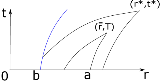
When we consider the initial-boundary value problem, as in Figure 1, with the 1-characteristic starting from , denoted by , as the left boundary curve, we further assume that the boundary data satisfy the following property.
Assumption 2.
Assume . There exists a uniform constant such that
| (1.6) |
for any , where .
We know that inequalities (1.5) form an invariant domain holding for any time before singularity formation, see [7]. This similar property was first established by Chen in [14] for studying the entropy solution. So there will be a uniform upper bound on and .
Now we define the rarefactive and compressive waves for smooth solutions. Here smooth solutions always mean solutions in this paper.
Definition 1.1.
For definitions of both rarefactive and compressive waves, we include and for convenience.
The main results of this paper, for (1.1)-(1.3) satisfying Assumption 1 and 2, can be summarized as:
- 1.
-
2.
When the initial data include some strong compression, i.e. at some point or is very negative, singularity form in finite time: Theorem 6.3.
Since physically , we note that the Assumption 1 is satisfied for the entire half line , only when .
For the existence result, we consider both vacuum and non-vacuum cases at the origin. When , we assume that Assumption 1 is satisfied for the entire half line . For the non-vacuum case, we apply the affine solution, inspired by [7, 41], to fill a small neighborhood centered at the origin.
It is well-known that the main difficulty in establishing the global existence of smooth solutions is obtaining the a priori estimates of the solution and its gradient variables. First, an appropriate density lower bound estimate is needed to extend the local solution to the entire domain. Fortunately, this result has already been proved in [7], following by the idea used in [8]. Also see [13, 9]
The key estimate on gradient variables comes from two invariant domains in the plane, by studying the Riccati equations on and . On the other hand, the proof of singularity formation result heavily relies on the Riccati equations too. These equations will be used for the future study in other cases, not satisfying the Assumption 1, including the imploding subsonic waves.
The rest of the paper is organized as follows. In Section 2, we calculate the rarefactive and compressive characters. In Section 3, we derive the Riccati equations of the R/C characters. In Section 4, we establish the invariant domains for the smooth solution itself and the R/C characters. Moreover, we deduce a density lower bound estimate which depends only on the time and is independent of the spatial variable . In Section 5, we prove the global existence of -solution on the entire domain for rarefaction initial data. Finally, in Section 6, we show that, when the initial data include strong compression somewhere, the smooth solution can form singularity in a finite time.
2 The R/C characters
When , we use the sound speed
as the variable to take the place of . So, for smooth solutions, equations (1.1)-(1.2) can be written as
| (2.1) | ||||
| (2.2) |
with characteristic speeds
| (2.3) |
Introduce the Riemann variables and
| (2.4) |
Then we have the governing equations of
| (2.5) | ||||
| (2.6) |
Now we calculate the R/C characters and defined in (1.4). By (1.2) and the definition of , it is easy to calculate that, when and ,
where in the last step, we used
Similarly, when and ,, we have
In summary, when , and , for smooth solution, (1.4) is equivalent to
| (2.7) | |||
| (2.8) |
We remark that and are different from derivatives of Riemann variables, i.e. , .
3 Riccati equations
Now, we can derive the following Riccati equations for Euler equations.
Lemma 3.1.
Equations (3.1) and (3.3) are homogeneous, i.e. the right hand sides of (3.1) and (3.3) vanish when and both vanish. This is because we find and from the stationary solution, so when , their time derivatives also vanish. This property is crucial for us to prove several important invariant domains on gradient variables, which serve as our basis to study the existence of classical solutions and singularity formation.
Proof.
We first calculate the equation of by (2.7)
| (3.6) |
It follows by (2.1)-(2.2) that
| (3.7) |
and
| (3.8) |
| (3.9) |
Substituting (3.9) into (3.6) yields
For future use, we calculate and :
| (3.13) |
Therefore, by (2.1), we know that
| (3.14) |
which yields
| (3.15) |
Via a similar computation, we arrive at
| (3.16) |
4 Invariant domains
Before studying the solution in the whole domain , we first consider the following two problems on the domain in the -plane.
Definition 4.1.
We define two problems for (1.1)-(1.3).
-
•
Problem 1: Cauchy problem on domain of dependence on the -plane with base and for any , i.e. domain to the right of the 2-characteristic starting at .
-
•
Problem 2: Boundary value problem on the half Goursat problem on the domain on the -plane to the right of the 1-characteristic boundary starting at the point .
Later, using results on these two problems, we will prove the global existence of some classical solution on the entire half line . The construction is divided into two cases: and . Specifically, to construct a smooth solution with positive density at the origin, we apply the affine solution to fill the domain between the line and the 1-characteristic curve .

We first review an invariant domain on or equivalently on .
Theorem 4.2.
For , when the initial data satisfy the initial Assumption 1, any smooth solution of Problem 1 in the domain of dependence based on , with , satisfies
| (4.1) |
If the initial Assumption 1 and the boundary Assumption 2 are satisfied, then inequality (4.1) holds for any smooth solution of Problem 2 in the domain of dependence . Moreover, when , assume initially (1.5) holds for any and then the inequality (4.1) holds on the domain , with .
Proof.
For Problem 1, one can directly use the proof of Theorem 2.1 in [7] to obtain that the inequality (4.1) holds on the domain . We here give the proof of (4.1) to Problem 2 for the sake of completeness.
Thanks to the result of Problem 1, it suffices to verify (4.1) on the region bounded by and the 2-characteristic starting at point . Recalling the definitions of and , we only need to prove the following inequalities
| (4.2) |
on . We shall show (i.e. ) for at the end of this section.
Using (4.4), we next prove that the set is an invariant domain in Problem 1 and 2 in the following lemma.
Lemma 4.3.
Remark 4.4.
The idea of proof is base on the observation that is an invariant domain on the -plane. In fact, when and , , and when and , . So it is very easy to prove that, is an invariant domain using the similar method as in [7] or [8]. To obtain a more general version of invariant domain on , one needs to introduce a small perturbation .
Proof.
According to Theorem 4.2 and the precise expressions of , we know that there exists a positive constant such that
| (4.5) |
where depends on . Here we note that
and
| (4.6) |
which have positive upper bounds when .
Set and is an arbitrary small number such that . We now introduce two new variables for
In view of Lemma 3.1, one can derive the governing system of
| (4.7) |
and
| (4.8) |
By the choice of and , it is observed that
| (4.9) |
We now apply the contradiction argument to show is an invariant domain for . We first see by the initial or initial boundary value conditions that () and () for Problem 2. Suppose that the region is not an invariant domain; that is, there exists some time, such that or , at some point with . Because the wave speed is bounded on , then we can find the characteristic triangle with vertex and lower boundary on the initial line , denoted by . If for Problem 2, then is the characteristic quadrangle bounded by the 1- and 2-characteristics through , lower boundary on the initial line , and part of curve . See Figure 1.
In turn, we can find the first time such that or in .
Case 1:
At time , , and .
Case 2:
At time , , and .
In this case, we consider the interval and apply (4) and (4.9) again to obtain
and subsequently
One integrates the above along the 2-characteristic from to to acquire
where if , while is determined by if . In view of the initial and boundary value conditions, we observe that cannot be finite, which leads a contradiction.
Hence we have
for and any satisfying . By the arbitrariness of , one obtains
The proof of the lemma is complete. ∎
Next, we prove another invariant domain on the upper bounds of and , which show that the maximum rarefaction is bounded if it is initially bounded. A similar invariant domain was first established for the 1-d problem in [8, 9], then extended to the radially symmetric solution in [7]. Using the new coordinates, we get a much better estimate in the following lemma than the one in [7].
Lemma 4.5.
Proof.
We first show two important relations:
| (4.12) |
Once we proved (4.12), to explain the idea, we see that on the right boundary of domain on the -plane, . So , since . Similarly, we know on the upper boundary of the invariant domain. By Lemma 4.3, this domain is invariant on time.
Now we prove (4.12). It suggests by (4.1) that
| (4.13) |
and
| (4.14) |
on . We rewrite the expressions of and in Lemma 3.1 as
and
Hence one calculates
Here we note by (4.14) that the term is well-defined.
Then we prove , for any time , by contradiction. As in the previous Lemma 4.3, we may assume that there exists a characteristic triangle tip or a characteristic quadrangle tip at such that or at , but and in the characteristic triangle or characteristic quadrangle.
Without loss of generality, we assume and at . It is observed that
at the vertex , which violates our assumption that in the characteristic triangle or characteristic quadrangle. We can find a similar contradiction when and at . Hence, we prove the lemma. ∎
We now derive a time-dependent density positive lower bound. A density lower bound was provided in Theorems 4.1 and 4.2 in [7] by studying the solution in the Lagrangian coordinates. Here, we give a much better and cleaner lower bound on density using our new Riccati system directly in the Euler coordinates and Lemma 4.5.
Lemma 4.7.
Let the assumptions in Lemma 4.5 hold. Moreover, suppose that the initial data satisfy
| (4.15) |
Then, for , the smooth solution on for Problem 1 and 2 satisfies
| (4.16) |
where is a positive constant depending on , and
Proof.
We set and apply the definitions of to obtain
| (4.17) |
which together with (3.16) and (3.15) gives
| (4.18) |
By the relationship between and , we calculate
| (4.19) |
from which one has
| (4.20) |
Recalling (4.13) and (4.14), we have
| (4.21) |
Here we used the fact for any point in .
Let be the curve defined by
| (4.22) |
for any point and . We denote the intersection point of and the initial line or boundary curve by . Then
| (4.23) |
which indicates that
| (4.24) |
Integrating (4.20) along and applying Lemma 4.5, (4.21) and (4.24), we conclude that
| (4.25) |
where , and
| (4.26) |
The proof of the lemma is finished. ∎
5 Global existence result on the entire half line
The first goal of this section is to show that the existence of solution in in Problem 1 and 2, when the initial data include only rarefaction, i.e. when . For Problem 2, we also assume that there is only rarefaction on the boundary , i.e. for .
Then, letting , we can construct the global existence result on , with at the origin.
We will also construct some global classical solutions with positive density, by adding some special initial data on .
To prove these results, we need to use the bound in (4.1), the density lower bound in (4.16) and bound for and .
5.1 Global existence for Problem 1 and 2
For Problem 1, we have the following existence theorem
Theorem 5.1.
Let the initial data satisfy Assumption 1 and . Suppose that
| (5.1) |
with
| (5.4) |
Here is a positive constant and . Then, for , Problem 1 admits a global solution on domain of dependence on the -plane with base and for any . Moreover, the solution satisfies
| (5.5) |
for some positive constant , and
| (5.6) |
Here .
Proof.
The proof of the theorem is based on the classical framework of Li [27] by extending the local smooth solution to global domain. The local existence of smooth solution to Problem 1 follows from the classical results, see, e.g. Li and Yu [28] or Bressan [2]. In order to extend the local solution to a global one, it suffices to establish the a priori estimates of the solution on the domain . Actually, by examining the proof process of local classical solution in [28], the existence time of the smooth solution depends only on the norm and the norm , where is the following set of functions
| (5.7) |
and , . See Remark 4.1. in Chapter 1 in [28]. From the above and the a priori estimates in Section 4, we know that, for any number and any time , the existence time depends only on and , which means that, for the fixed and , the local existence time is a constant. Hence we can solve a finite number of local existence problems to extend the solution in the region to the global region . By the arbitrariness of , we can obtain the smooth solution on the global region for any fixed . The properties of solution in (5.5) and (5.6) can be acquired directly by the results in Section 4. ∎
For Problem 2, we have
Theorem 5.2.
Let the initial conditions of in Theorem 5.1 hold. Let be a smooth increasing curve. Assume that the boundary value on satisfies Assumption (2) and
| (5.10) |
where with for any . Moreover, the function satisfies
| (5.11) |
where
| (5.12) |
and is a positive constant. In addition, suppose that the following compatibility conditions hold
| (5.15) |
Then, for , Problem 2 admits a global solution on the domain bounded by the initial line and the curve for any . Moreover, the solution satisfies
| (5.16) |
for some positive constant , and
| (5.17) |
Here .
Proof.
Based on Theorem 5.1, it suffices to consider the global existence of the Goursat type boundary value problem on the domain which is bounded by the 1-characteristic and the 2-characteristic starting from point . Here the curve is determined in solving Problem 1. Moreover, the boundary data on satisfies (5.5) and (5.6). For this typical Goursat problem, we can also utilize the classical framework of Li [27] to extend the local smooth solution to global domain. The local existence time of the smooth solution in Li and Yu [28] depends only on the norm and the norms of on the boundaries and . Thanks to the a priori estimates in Section 4, the existence time still depends only on the number and the time . By solving a finite number of local Goursat and Cauchy problems, we can acquire the global existence of smooth solution on the domain . Due to the arbitrariness of , we obtain the smooth solution over the entire region , which completes the proof of the theorem. ∎
5.2 Global existence on the entire half line
Let’s start to construct the global solution on the entire half line . We further assume that the boundary condition at the origin, which is a reasonable physical assumption.
For the data of the density at the origin, a direct and simple choice is , which makes that the initial assumption (1.5) is satisfied on the entire half line . For this choice, one can apply the results in Theorem 5.1 to construct the global smooth solution. Suppose that the initial conditions in Theorem 5.1 hold for any . Moreover, we assume that, when approaches 0, the limits of and exist and are nonnegative. For any point with , we let small enough such that is in the corresponding domain . Here we used the result in [7] that the characteristic starting from must be . Hence we obtain the smooth solution on the entire domain .
Thus we have
Theorem 5.3.
Let the initial data satisfy Assumption 1 and , , for . Suppose that
| (5.18) |
where and are given in (5.4), and is a positive constant. Here and which are assumed to exist. Then, for , the radially symmetric Euler equations (1.1)-(1.3) admit a global solution on the entire domain . Moreover, the solution satisfies , and
| (5.19) |
and
| (5.20) |
There is another choice that the density is positive at the origin. Inspired in [41] and [7], we may construct a smooth solution satisfying affine motion close to and then combine it with the smooth solution obtained in Problem 2 to acquire a global solution on the entire domain .
In order to proceed, we start from the affine motions
| (5.21) |
In material coordinates, the velocity associated to this motion is
| (5.22) |
from which we get the material time derivative of the velocity
| (5.23) |
We take the material derivative on and employ the equation (1.1) to achieve
| (5.24) |
Thus there holds
| (5.25) |
which leads to
| (5.26) |
where is the initial value. Notice that the equation (1.2) can be rewritten as
| (5.27) |
which together with (5.23) and (5.26) yields
| (5.28) |
Hence we could separate the equations for and as
| (5.29) |
It follows directly by the second equation of (5.29) that
| (5.30) |
where is a positive constant. Moreover, for affine motion , one has , which implies that . Thus we could have the ODE problem
| (5.31) |
where is the initial velocity. This problem equals to
| (5.32) |
It is obvious that for
| (5.33) |
By the standard ODE theory, we know that there exists a global unique solution for problem (5.32), which equivalently gives a global unique solution for problem (5.31).
Let’s construct the central affine solution. For any fixed and , we know by (5.22) and (5.30) that
| (5.34) |
which implies there exists such that
| (5.35) |
Thus we consider the initial data that satisfies the following assumption
Assumption 3.
Assume that the initial data satisfy that when , and (1.5) holds when .
Denote the domain of dependence with base by . We know that the right boundary of is the -characteristic starting from , that is . It is easy to see by (5.35) that this boundary is moving outward, i.e. away from the origin, as increases. Inside the region , we have
| (5.36) |
which together with (5.30) and (5.33) leads to the uniform upper bound of
| (5.37) |
Now we seek suitable conditions such that the above constructed affine solution satisfy the boundary condition of Theorem 5.2 on the -characteristic . By the expression of the affine solution in (5.36), one has
| (5.38) |
for , from which we obtain
| (5.41) |
It is easy to see that , which together with the equation of (2.6) yields that is increasing along the curve . Thus
In view of (5.41) and the properties of , if
| (5.42) |
one then has and then on by . We next differentiate and in (5.41) with respect to to acquire
| (5.45) |
According to the expressions of and in (2.7) and (2.8), we find that, if on , then there holds . To get it, by the expression of in (5.45) and the relation , it suffices to
| (5.46) |
Due to the monotonic increasing property of on the left-side of inequality (5.46), we only need
| (5.47) |
by . On the other hand, one recalls the properties of to obtain
Hence to ensure on , we only need
| (5.48) |
For the value , we calculate by (5.45) and the expression of
| (5.49) |
from which one has provided that
| (5.50) |
Summing up (5.42), (5.48) and (5.50), we see that if the parameters and satisfy
| (5.51) |
and
| (5.52) |
then there hold
| (5.55) |
Note that the function is strictly monotonically increasing along , we can obtain for . Moreover, one recall the equation of in (3.1) with on to easily achieve . We next derive the upper bound of . It suggests by (5.33) and (5.45) that
| (5.56) |
which together with (5.37) and (2.7) arrives at
| (5.57) |
where the positive constant depends only on . In addition, by the construction of the affine solution in (5.36), it is easy to check that all compatibility conditions in (5.15) are satisfied. Hence, all conditions of Theorem 5.2 hold provided that the parameters and satisfy (5.51) and (5.2).
Therefore, we have
Theorem 5.4.
Let the initial data satisfy Assumption 3 and . Suppose that the positive parameters and satisfy (5.51) and (5.2), where , , . Then, for , the radially symmetric solution of Euler equations (1.1)-(1.3) admit a global solution on the entire domain . Moreover, the solution takes the form in (5.36) on the left-hand region of the 1-characteristic starting from , and satisfies (5.16) and (5.17) on its right-hand region.
Proof.
Based on the above analysis and the result in Theorem 5.2, we just need to check the existence of parameters and such that (5.51) and (5.2) can be satisfied simultaneously. Indeed, for any fixed positive constant , we can freely choose the parameter as long as the following relationship holds
Thus the constants and satisfy
which is (5.51). Now the three terms in the right-hand side of (5.2) are fixed constants. Then we choose sufficiently large such that it is greater than these three constants. Hence (5.2) is fulfilled. Furthermore, the inequality (5.35) follows directly from (5.2). The proof of the theorem is complete. ∎
6 Singularity formation
To prove the singularity formation when the initial data include strong compression somewhere, we need to further decouple the system on and . In order to do that, we first show the following lemma.
Lemma 6.1.
Proof.
Specifically, we take in (6.1) and (6.2) and denote
| (6.5) |
to obtain
| (6.6) | |||
| (6.7) |
We note that these two equations are decoupled in its leading quadratic order term.
To prove the desired singularity formation result, one difficulty is to control the last term in (6.6) and (6.7). We cannot directly use the upper bound of and in Lemma 4.5 and the density lower bound in Lemma 4.7, since our initial and might be negative somewhere. Instead, we use the upper bound on gradient variables to re-establish the density lower bound which do not require the initial conditions and .
We first take in (6.1) and (6.2) and denote
| (6.8) |
to acquire
| (6.9) | ||||
| (6.10) |
Recalling Theorem 4.2 and (4.6), one has for
| (6.11) |
for some positive constant depending on .
Lemma 6.2.
Proof.
The proof is also based on the contradiction argument. In view of the construction of and (6.8), (6.14), we first achieve that the initial or boundary data fulfill
Assume that there exists some time, such that or , at some point with . Then there exists a characteristic triangle tip or a characteristic quadrangle tip at such that or at , but and in the characteristic triangle or characteristic quadrangle. Without loss of generality, we assume and and on . Thus one first has
On the other hand, we apply (4.12), (6.11) and (6.13) to obtain
| (6.16) |
which yields a contradiction. The proof of the lemma is finished. ∎
Now thanks to (6.8), (6.15) and (4.1), we find that for
| (6.17) |
and then by (6.5)
| (6.18) |
Putting (6.17) into (4.20) and employing (4.21) arrives at
| (6.19) |
We integrate (6) along and utilize (4.24) to deduce
| (6.20) |
Based on the density lower bound in (6.20), we now derive the singularity formation result. We first rewrite (6.6) and (6.7) as
| (6.21) | ||||
| (6.22) |
We want to prove that when the initial or is less than some threshold , then we always have
| (6.23) |
or
| (6.24) |
by which, we can estimate the blowup time. In fact, integrating (6.23) along the 1-characteristic and assuming for any time before blowup, we have
| (6.25) |
where is the corresponding 1-characteristic curve and . Thanks to the lower bound of in (4.16), one obtains
| (6.26) |
subsequently
| (6.27) |
where
with . Combining (6.25) and (6.27) and using the fact , we know that blowup happens not later than
| (6.28) |
provided that is large enough. It is easy to see that as .
Noting , the boundedness of and in (4.5), the upper bound of in (6.18), and the density lower bound in (6.20), we can choose large enough such that
when and , and
when and . On the other hand, choose large enough, such that, if , then the blowup time is less than . In addition, if for sufficiently large , we can similarly show the blowup time is finite.
In a summary, we proved the following singularity formation theorem:
Theorem 6.3.
We consider global solution with initial data satisfying the Assumption 1 on , with . Assume and there exists , such that
For Problem 2, we also suppose that the boundary date satisfy the Assumption 2 on . Then there exists a constant , depending on and , such that, if
then singularity forms before time .
Acknowledgements
The first and second author were partially supported by National Science Foundation (DMS-2008504, DMS-2306258), the third author was partially supported by National Natural Science Foundation of China (12171130, 12071106), the fourth author was partially supported by National Science Foundation (DMS-2206218).
References
- [1] S. Alinhac, Blowup for Nonlinear Hyperbolic Equations, Progress in Nonlinear Differential Equations and Their Applications 17, Birkhäuser, Boston, 1995.
- [2] A. Bressan, Hyperbolic systems of conservation laws: the one-dimmensional Cauchy problem, Oxford Lecture Ser. Math. Appl., Oxford Univ. Press, Oxford, 2000.
- [3] T. Buckmaster, T. Drivas, S. Shkoller and V. Vicol, Simultaneous development of shocks and cusps for 2D Euler with azimuthal symmetry from smooth data, Ann. PDE, 8 (2022), no. 2, pp. 199.
- [4] T. Buckmaster, S. Shkoller and V. Vicol, Formation of shocks for 2d isentropic compressible Euler, Commun. Pure Appl. Math., 75 (2022), no. 9, 2069–2120.
- [5] T. Buckmaster, S. Shkoller and V. Vicol, Shock formation and vorticity creation for 3d Euler, Commun. Pure Appl. Math., 76 (2023), no. 9, 1965–2072.
- [6] T. Buckmaster, S. Shkoller and V. Vicol, Formation of point shocks for 3D compressible Euler, Commun. Pure Appl. Math., 76 (2023), no. 9, 2073–2191.
- [7] H. Cai, G. Chen and T. Wang, Singularity formation for radially symmetric expanding wave of Compressible Euler Equations, SIAM J. Math. Anal., 55 (2023), no. 4, 2917–2947.
- [8] G. Chen, Optimal time-dependent lower bound on density for classical solutions of 1-D compressible Euler equations, Indiana Univ. Math. J., 66 (2017), no. 3, 725–740.
- [9] G. Chen, Optimal time-dependent density lower bound for nonisentropic gas dynamics, J. Differential Equations, 268 (2020), no. 7, 4017–4028.
- [10] G. Chen, G.Q. Chen and S. Zhu, Formation of singularities and existence of global continuous solution for the compressible Euler equations, SIAM J. Math. Anal., 53 (2021), no. 6, 6280–6325.
- [11] G. Chen and R. Young, Shock-free solutions of the compressible Euler equations, Arch. Ration. Mech. Anal., 217 (2015), no. 3, 1265–1293.
- [12] G. Chen, R. Young and Q. Zhang, Shock formation in the compressible Euler equations and related systems, J. Hyperbolic Differ. Equ., 10 (2013), no. 1, 149–172.
- [13] G. Chen, R. Pan and S. Zhu, Singularity formation for compressible Euler equations, SIAM J. Math. Anal., 49 (2017), no. 4, 2591–2614.
- [14] G.Q. Chen, Remarks on spherically symmetric solutions of the compressible Euler equations, Proc Roy. Soc. Edinb. A, 127 (1997), no. 2, 243–259.
- [15] S. Chen, Z. Xin and H. Yin, Formation and Construction of Shock Wave for Quasilinear Hyperbolic System and its Application to Inviscid Compressible Flow, Research Report, IMS, CUHK, 1999.
- [16] D. Christodoulou, The Shock Development Problem, EMS Monographs in Mathematics, European Mathematical Society (EMS), Zürich, 2019.
- [17] D. Christodoulou and S. Miao, Compressible Flow and Euler’s Equations, Surveys of Modern Mathematics 9, International Press, Somerville, MA; Higher Education Press, Beijing, 2014.
- [18] R. Courant and K. Friedrichs, Supersonic flow and shock waves, Wiley-Interscience, New York, 1948.
- [19] M. Disconzi, C. Luo, G. Mazzone and J. Speck, Rough sound waves in 3D compressible Euler flow with vorticity, Sel. Math. New Ser., 28 (2022), article number 41.
- [20] M. Grassin, Global smooth solutions to Euler equations for a perfect gas, Indiana Univ. Math. J., 47 (1998), no. 4, 1397–1432.
- [21] P. Godin, The lifespan of a class of smooth spherically symmetric solutions of the compressible Euler equations with variable entropy in three space dimensions, Arch. Ration. Mech. Anal., 177 (2005), no. 3, 479–511.
- [22] M. Hadi and J. Jang, Expanding large global solutions of the equations of compressible fluid mechanics, Inventiones Mathematicae, 214 (2018), no. 3, 1205–1266.
- [23] F. John, Formation of singularities in one-dimensional nonlinear wave propagation, Comm. Pure Appl. Math., 27 (1974), no. 3, 377–405.
- [24] D. Kong, Formation and propagation of singularities for 2x2 quasilinear hyperbolic systems, Trans. Amer. Math. Soc., 354 (2002), no. 4, 3155–3179.
- [25] G. Lai and M. Zhu, Global-in-time classical solutions to two-dimensional axisymmetric Euler system with swirl, Commun. Math. Sci., 21 (2023), No. 3, 829–857.
- [26] P. Lax, Development of singularities of solutions of nonlinear hyperbolic partial differential equations, J. Math. Phys., 5 (1964), no. 5, 611–614.
- [27] T.T. Li, Global classical solutions for quasilinear hyperbolic systems, Wiley, New york, 1994.
- [28] T.T. Li and W.C. Yu, Boundary Value Problems for Quasilinear Hyperbolic Systems, Duke University, 1985.
- [29] T.T. Li, Y. Zhou and D.X. Kong, Global classical solutions for general quasilinear hyperbolic systems with decay initial data, Nonlinear Analysis, Theory, Methods Applications, 28 (1997), no. 8, 1299–1332.
- [30] T.P. Liu, The development of singularities in the nonlinear waves for quasi-linear hyperbolic partial differential equations, J. Differential Equations, 33 (1979), no. 1, 92–111.
- [31] J. Luk and J. Speck, Shock formation in solutions to the 2D compressible Euler equations in the presence of non-zero vorticity, Invent. Math., 214 (2018), no. 1, 1–169.
- [32] J. Luk and J. Speck, The stability of simple plane-symmetric shock formation for 3D compressible Euler flow with vorticity and entropy, arXiv: 2107.03426, 2021.
- [33] L. Magali, Global smooth solutions of Euler equations for Van der Waals gases, SIAM J. Math. Anal., 43 (2011), no. 2, 877–903.
- [34] I. Neal, C. Rickard, S. Shkoller and V. Vicol, A new type of stable shock formation in gas dynamics, arXiv: 2303.16842, 2023.
- [35] I. Neal, S. Shkoller and V. Vicol, A characteristics approach to shock formation in 2D Euler with azimuthal symmetry and entropy, arXiv: 2302.01289, 2023.
- [36] S. Parmeshwar, M. Hadi and J. Jang, Global expanding solutions of compressible Euler equations with small initial densities, Quart. Appl. Math., 79 (2021), no. 2, 273–334.
- [37] C. Rickard, Global solutions to the compressible Euler equations with heat transport by convection around Dyson’s isothermal affine solutions, Arch. Rat. Mech. Anal., 241 (2021), no. 2, 947–1007.
- [38] C. Rickard, M. Hadi and J. Jang, Global existence of the nonisentropic compressible Euler equations with vacuum boundary surrounding a variable entropy state, Nonlinearity, 34 (2020), no. 1, 33.
- [39] S. Shkoller and T. Sideris, Global existence of near-affine solutions to the compressible Euler equations, Arch. Rat. Mech. Anal., 234 (2019), no. 1, 115–180.
- [40] T. Sideris, Formation of singularities in three-dimensional compressible fluids, Commun. Math. Phys., 101 (1985), no. 4, 475–485.
- [41] T. Sideris, Global existence and asymptotic behavior of affine motion of 3D ideal fluids surrounded by vacuum, Arch. Ration. Mech. Anal., 225 (2017), no. 1, 141–176.
- [42] C. Zhu, Global smooth solution of the nonisentropic gas dynamics system, Proc. Roy. Soc. Edinb. Sect. A, 126 (1996), no. 4, 768–775.