Probing Three-Dimensional Magnetic Fields: III - Synchrotron Emission and Machine Learning

Abstract

Synchrotron observation serves as a fundamental tool for studying magnetic fields in various astrophysical settings, yet its ability to unveil three-dimensional (3D) magnetic fields—including plane-of-the-sky orientation, inclination angle relative to the line of sight, and magnetization—remains largely underexplored. Inspired by the latest insights into anisotropic magnetohydrodynamic (MHD) turbulence, we found that synchrotron emission’s intensity structures inherently reflect this anisotropy, carrying detailed information about 3D magnetic fields. Capitalizing on this foundation, we integrate a machine learning approach-Convolutional Neural Network (CNN)-to extract this latent information, thereby facilitating the exploration of 3D magnetic fields. The model is trained on synthetic synchrotron emission maps, derived from 3D MHD turbulence simulations encompassing a range of sub-Alfvénic to super-Alfvénic conditions. We show that the CNN model is physically interpretable and the CNN is capable of reconstructing 3D magnetic field topology and assessing magnetization. In addition, we test our methodology against noise and resolution effects. We show that this CNN-based approach maintains a high degree of robustness in tracing 3D magnetic fields, even when the low spatial frequencies of the synchrotron image are absent. This renders the method particularly suitable for application to interferometric data lacking single-dish measurements

1 Introduction

Synchrotron radiation, emanating from relativistic electrons gyrating around magnetic field lines (Rybicki & Lightman, 1979; Condon, 1992), is a fundamental probe of magnetic fields in diverse astronomical settings (Ginzburg & Syrovatskii, 1965; Sun et al., 2008; Planck Collaboration et al., 2016a; Govoni et al., 2019; Wang et al., 2020; Heywood et al., 2022; Hu et al., 2020, 2024b). This radiation not only facilitates the estimation of magnetic field strengths at equilibrium (Chevalier & Luo, 1994; Arshakian et al., 2009; Yusef-Zadeh et al., 2022, 2024), which is pivotal for elucidating cosmic ray acceleration mechanisms (Jokipii, 1966; Bell, 1978; Bykov et al., 2012; Caprioli & Spitkovsky, 2014; Bonafede et al., 2014; Xu & Lazarian, 2022; Xu, 2022), but it also allows the determination of magnetic field orientations (Beck, 2001, 2015; Planck Collaboration et al., 2016a; Zhang et al., 2019a; Guan et al., 2021). This is crucial for understanding different physics across scales, from large-scale galaxy clusters (Govoni & Feretti, 2004; Brunetti & Jones, 2014; Stuardi et al., 2021; Hu et al., 2024b), galaxies (Beck, 2001, 2015), to small- scale individual supernova remnants (McLean et al., 1983; Xiao et al., 2008, 2009; Reynolds et al., 2012). Despite its critical role, our comprehension of synchrotron radiation and the magnetic field insights it can offer is still evolving.

Extracting three-dimensional (3D) magnetic field information from synchrotron radiation poses a substantial challenge. Polarized synchrotron emission offers two-dimensional (2D) insights into the magnetic field orientation within the plane of the sky (POS) (Rybicki & Lightman, 1979; McLean et al., 1983; Beck, 2001; Xiao et al., 2009; Reynolds et al., 2012; Beck, 2015; Planck Collaboration et al., 2016a; Zhang et al., 2019a; Guan et al., 2021). However, the inclination angle of the magnetic field relative to the line of sight (LOS) remains elusive. The scenario is further complicated by the Faraday rotation effect, which alters the intrinsic polarization angle of the emission sources (Haverkorn, 2007; Taylor et al., 2009; Oppermann et al., 2012; Xu & Zhang, 2016; Tahani et al., 2019). Consequently, not only is accurately measuring the POS magnetic field from synchrotron polarization challenging, but tracing the actual 3D magnetic field structure becomes a formidable task.

Recent advancements have unlocked the potential of using anisotropy in synchrotron radiation as a means to trace 3D magnetic fields. The theory that relates the anisotropy of synchrotron radiation with the properties of magnetohydrodynamic (MHD) turbulence (Goldreich & Sridhar, 1995; Lazarian & Vishniac, 1999), turbulence was formulated in Lazarian & Pogosyan (2012). The anisotropy means the observed synchrotron intensity structures tend to elongate along the magnetic field lines intersecting them. Based on this property, Lazarian et al. (2017) introduced the Synchrotron Intensity Gradients (SIG) to trace the POS magnetic field orientation (Lazarian et al., 2017; Hu et al., 2024b). The technique was demonstrated to be accurate for application under both sub-Alfvénic and super-Alfvénic conditions, notably within galaxy clusters as demonstrated by Hu et al. (2024b). Crucially, subsequent research by Hu et al. (2021a) and Hu et al. (2024a) has shown that the observed anisotropy in the POS contains information on the underlying 3D magnetic field structures. This revelation stems from the fact that the anisotropy, or elongation along the magnetic field line, is inherently a 3D phenomenon. Therefore, the observed POS anisotropy, or the topology of synchrotron intensity structures, is influenced by the projection effect, which is determined by the inclination angle of the magnetic field with respect to the LOS and the magnetization level of the medium.

Given these theoretical considerations, the observed structure of synchrotron emission intrinsically encompasses information pertinent to 3D magnetic fields. In this study, we propose the employment of a machine learning paradigm—specifically, Convolutional Neural Networks (CNNs; LeCun et al. 1998)—to discern spatial features or topology within the synchrotron intensity maps, thereby facilitating the measurement of 3D magnetic fields. This includes determining the orientation of the magnetic field within the POS, ascertaining the magnetic field’s inclination angle, and assessing the overall magnetization. A similar methodology employing CNNs for 3D magnetic field tracing, based on spectroscopic data, has been previously proposed by Hu et al. (2024a), affirming the CNN’s capability to identify magnetic-field-specific spatial topologies or features from substantial training datasets, thereby yielding precise measurements.

Crucially, our approach transcends mere algorithmic application; we aim to rigorously analyze the synchrotron intensity structures to understand which features are indicative of magnetic field properties, why these features are significant, and the fundamental physical principles they represent. This strategy not only deepens our understanding of CNN’s efficacy in producing 3D magnetic field mappings but also the relation between observed synchrotron structures and magnetic field properties. For the CNN training, we utilize 3D MHD subsonic simulations that encompass a range of magnetization levels, ranging from sub-Alfvénic conditions (i.e., strong magnetic fields), through trans-Alfvénic, to super-Alfvénic scenarios (i.e., weak magnetic fields). These simulations are subsequently post-processed to create synthetic synchrotron observations.

This paper is organized as follows. In § 2, we outline the fundamental aspects of MHD turbulence anisotropy observed in synchrotron emissions and their association with 3D magnetic field orientation and overall magnetization. § 3 provides a comprehensive description of the 3D MHD simulations and the synthetic observations utilized in this study, alongside details of our CNN model. In § 4, we present the results derived from our numerical testing, offering insights into the efficacy and accuracy of the CNN model. § 5 delves into discussions surrounding the uncertainties and future prospects of employing machine learning techniques for astrophysical analysis. We conclude with a summary of our findings in § 6.

2 Theoretical consideration

2.1 Anisotropy in MHD turbulence

A significant advancement in our understanding of MHD turbulence was the introduction of the ”critical balance” condition, equating the cascading time, $(k_{\bot}\delta v_{l})^{-1}$, with the wave periods, $(k_{\parallel}v_{A})^{-1}$, as proposed by Goldreich & Sridhar (1995) (hereafter GS95). Here, $k_{\parallel}$ and $k_{\bot}$ denote the components of the wavevector parallel and perpendicular to the magnetic field, respectively. The term $\delta v_{l}$ refers to the turbulent velocity at scale $l$, and $v_{A}=B/\sqrt{4\pi\rho}$ represents the Alfvén speed, where $B$ is the magnetic field strength and $\rho$ is the gas mass density. It is essential to note that GS95’s analysis is grounded in a global reference frame, wherein the orientation of wavevectors is defined relative to the mean magnetic field.

Lazarian & Vishniac (1999) (hereafter LV99) subsequently demonstrated that the ”critical balance” condition also holds in a local reference frame, defined relative to the magnetic field intersecting an eddy at scale $l$. According to LV99, the process of turbulent reconnection of the magnetic field, occurring within one eddy turnover time, facilitates the mixing of magnetic field lines perpendicular to the magnetic field’s orientation. This mixing induces changes in fluid velocities perpendicular to the magnetic field lines, ensuring that the motion of eddies sized $l_{\bot}$ and oriented perpendicular to the local magnetic field direction is not suppressed. This implies that the perpendicular direction poses minimal resistance to turbulent cascading, which typically follows the Kolmogorov law.

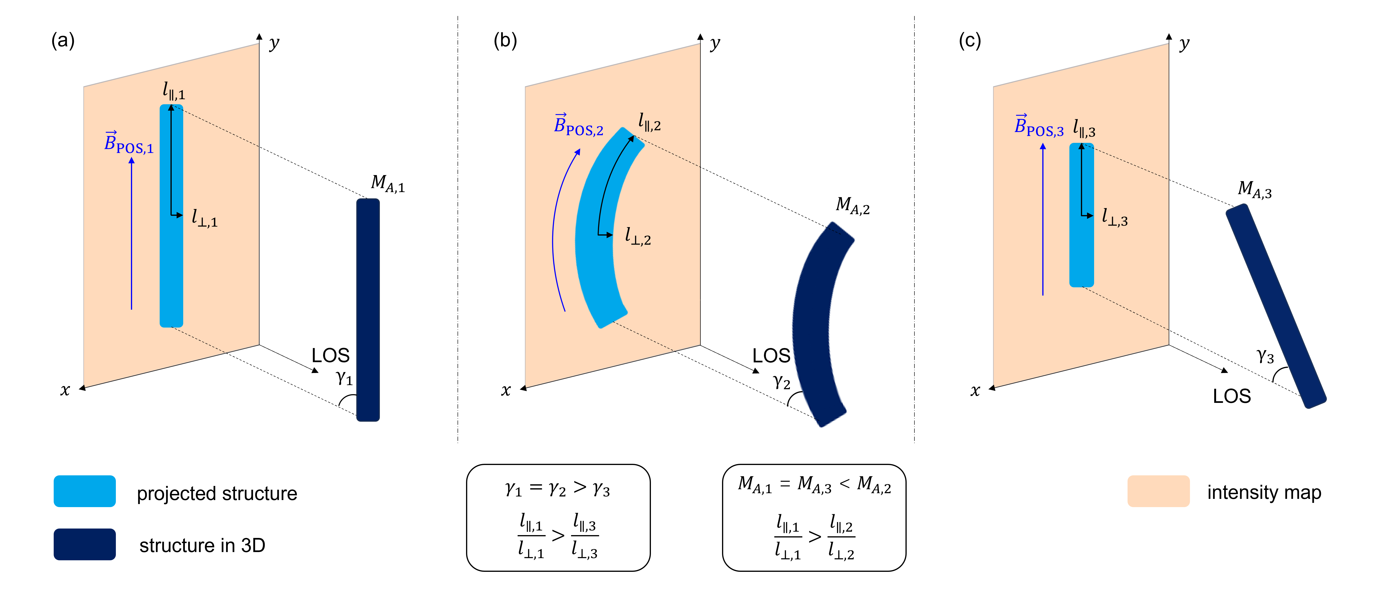
Figure 1: An Illustration of how the observed synchrotron intensity structures are regulated by the Alfvén Mach number $M_{A}$ and inclination angle $\gamma$. Within all three panels, these intensity structures elongate along the POS magnetic field direction where $l_{\parallel}>l_{\bot}$. Structures 1 and 2, depicted in panels (a) and (b), are projected onto the POS with identical inclination angles $\gamma_{1}=\gamma_{2}$, yet exhibit different magnetization with $M_{A,1}^{-1}>M_{A,2}^{-1}$. Notably, the anisotropy observed, represented as $l_{\parallel}/l_{\bot}$, in the weakly magnetized Structure 2 is less pronounced than in Structure 1. Structure 2 is less straightened because the weak magnetic field has more fluctuations. Comparatively, Structures 1 and 3—showcased in panels (a) and (c)—possess equivalent magnetization $M_{A,1}^{-1}=M_{A,3}^{-1}$, but divergent inclination angles with $\gamma_{1}>\gamma_{3}$. The observed anisotropy decreases with smaller $\gamma$, though it is crucial to note that the straightness of Structure 3 remains unaffected by this projection. Modified from Hu et al. (2024a).

Considering the ”critical balance” condition in the local reference frame: $\delta v_{l,\bot}l_{\bot}^{-1}\sim v_{A}l_{\parallel}^{-1}$ and the Kolmogorov relation (i.e., $\delta v_{l,\bot}=(\frac{l_{\bot}}{L_{\rm inj}})^{1/3}\delta v_{\rm inj}$, where $\delta v_{\rm inj}$ is the injection velocity at injection scale $L_{\rm inj}$ and $\delta v_{l,\bot}$ is turbulent velocity along the direction perpendicular to the magnetic field at scale $l$), one can get the scale-dependent anisotropy scaling (Lazarian & Vishniac, 1999):

$$l_{\parallel}=L_{\rm inj}(\frac{l_{\bot}}{L_{\rm inj}})^{\frac{2}{3}}M_{A}^{-4/3},~{}~{}~{}M_{A}\leq 1,$$ (1)

$$\delta v_{l,\bot}=\delta v_{\rm inj}(\frac{l_{\bot}}{L_{\rm inj}})^{\frac{1}{3}}M_{A}^{1/3},~{}~{}~{}M_{A}\leq 1,$$ (2)

where $l_{\bot}$ and $l_{\parallel}$ represent the perpendicular and parallel scales of eddies with respect to the local magnetic field, respectively. $M_{A}=\delta v_{\rm inj}/v_{A}$ is the Alfvén Mach number. This scaling relation has been demonstrated by numerical simulations (Cho & Vishniac, 2000; Maron & Goldreich, 2001; Cho & Lazarian, 2003; Kowal & Lazarian, 2010; Hu et al., 2021b, 2024c) and in-situ measurements in the solar wind (Wang et al., 2016; Matteini et al., 2020; Duan et al., 2021; Zhao et al., 2023).

Eq. 1 provides the scaling relation for velocity fluctuations and reveals the anisotropic nature of turbulent eddies (i.e., $l_{\parallel}\gg l_{\bot}$). In other words, the perpendicular velocity fluctuation is more significant than the parallel fluctuations at the same scale (Hu et al., 2021b). The corresponding relations for density and magnetic field fluctuations can be derived from the linearized continuity and induction equations in Alfvénic turbulence (Cho & Lazarian, 2003):

$$\delta\rho_{l} =\delta v_{l}\frac{\rho_{0}}{v_{A}}\mathcal{F}^{-1}(|\hat{\boldsymbol{k}}\cdot\hat{\boldsymbol{\xi}}|),$$ (3)

$$\delta B_{l} =\delta v_{l}\frac{B_{0}}{v_{A}}\mathcal{F}^{-1}(|\hat{\boldsymbol{B}}_{0}\cdot\hat{\boldsymbol{\xi}}|),$$ (4)

where $\rho_{0}$ and $B_{0}$ denote the mean density and mean magnetic field strength. $\hat{\boldsymbol{k}}$ and $\hat{\boldsymbol{\xi}}$ represent the unit wavevector and displacement vector, respectively. $\mathcal{F}^{-1}$ denotes an appropriate inverse Fourier transform. The density and magnetic field fluctuations induced by turbulence are still dominated by their perpendicular components.

In addition to the anisotropy, the topology of magnetic field lines is regulated by the magnetization. Within a domain of strong magnetization, magnetic field lines exhibit minimal deviation, attributed to subdued fluctuations, resulting in predominantly straightened topology. In contrast, a weaker magnetic field, signified by a higher $M_{A}$, amplifies directional fluctuations in the magnetic field. This enhancement leads to field lines adopting more curved formations (Yuen & Lazarian, 2020). Together with Eq.1, we have three important properties of MHD turbulence (Hu et al., 2024a):

1. Turbulent eddies predominantly stretch along the local magnetic field (i.e., $l_{\parallel}\gg l_{\bot}$), underscoring an anisotropy in velocity, density, and magnetic field structures.

2. The degree of anisotropy, quantified as $l_{\parallel}/l_{\bot}$, is intricately linked to the magnetization, represented by $M_{A}^{-1}$.

3. Changes in magnetization manifest distinctively in the magnetic field topology.

Note that for super-Alfvénic scenarios where $M_{A}\gg 1$, turbulence approaches isotropy, dominated by hydrodynamic turbulence. However, turbulence cascades energy from larger injection scales down to smaller scales and progressively diminishes turbulent velocity. This cascading process reaches a critical juncture at the transition scale $l_{A}=L_{\rm inj}/M_{A}^{3}$, where the magnetic field’s significance approaches that of turbulence (i.e., the Alfvén Mach number at $l_{A}$ becomes unity, as discussed by Lazarian 2006), heralding the onset of anisotropy.

2.2 Anisotropy in synchrotron emission

The intrinsic relationship between synchrotron emission and the density of relativistic electrons and magnetic fields (see Eq. 5), ensures that the anisotropy and magnetic field topology are naturally encoded in the observed synchrotron intensity structure. As illustrated in Fig. 1, the elongation in the projected intensity structure unveils the orientation of the POS magnetic field.

The degree of anisotropy in the intensity structure is more pronounced in environments with strong magnetization. However, it is crucial to recognize that the observed degree of anisotropy is influenced not only by the magnetization level but also by the projection effect, which is contingent upon the magnetic field’s inclination angle relative to the LOS. A lower anisotropy degree, i.e., $l_{\parallel}/l_{\bot}$, could stem from either weak magnetization or a minor inclination angle. This degeneracy, however, can be resolved through an examination of the topology of the projected intensity structure. Specifically, weaker magnetization correlates with a more pronounced curvature in both the magnetic field topology and the corresponding intensity structure. This change in topology cannot be induced by the projection effect. Therefore, insights into the degree of anisotropy combined with the topology of the projected intensity structure enable the determination of both the magnetization and inclination angle.

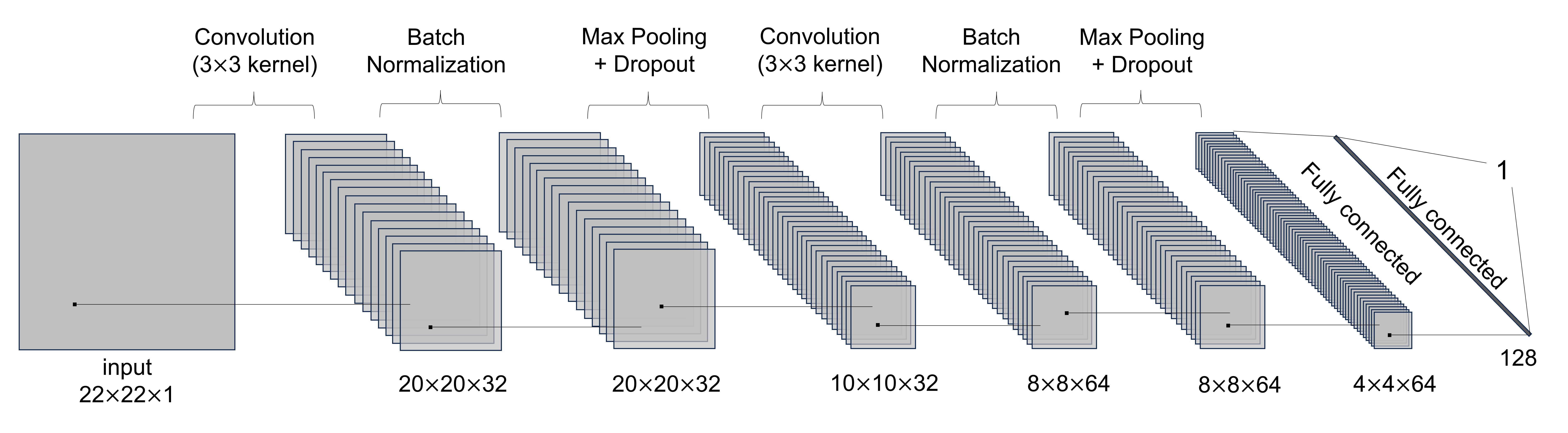
Figure 2: Architecture of the CNN-model. The input image is a $22\times 22$-cells map cropped from the synchrotron intensity map. The network outputs the prediction of the magnetic field’s POS orientation angle $\phi$, inclination angle $\gamma$, or the Alfvén Mach number $M_{A}$. Modified from Hu et al. (2024a).

3 Numerical method

3.1 Convolutional neural network (CNN)

3.1.1 CNN architecture

To construct a deep neural network (LeCun et al., 1998) to trace the 3D magnetic field from a synchrotron emission map, we adopt a CNN architecture similar to that used in Hu et al. (2024a). The CNN architecture, as illustrated in Fig. 2, consists of initial layers comprising a stack of convolutional layers followed by pooling and dropout layers. To facilitate faster convergence during the network training process using backpropagation of the loss and enhance the learning stability, we introduce a batch normalization layer following each convolution layer. After several iterations of convolution and pooling layers, we extract a compressed image feature, which is then processed by the fully connected layers to predict the desired properties. A detailed discussion of each layer’s function is given in Hu et al. (2024a). Such a CNN architecture has been proven to be effective in tracing 3D magnetic fields using spectroscopic observations.

3.1.2 Network Training

The trainable parameters within the CNN are optimized following a conventional neural network training approach, where the mean-squared error of the 3D magnetic field prediction acts as the training loss for backpropagation. This methodology is grounded in the foundational principles established by Rumelhart et al. (1986).

Random cropping: To bolster the CNN model’s ability to generalize, our training strategy includes diversifying the training dataset through data augmentation (van Dyk & Meng, 2001). One effective technique is random cropping (Takahashi et al., 2018), which involves generating smaller patches of size $22\times 22$ cells from the input images. This approach not only expands the dataset but also introduces a variety of perspectives within the data, thereby enhancing the model’s exposure to different features present in the synchrotron emission maps. The size of $22\times 22$ cells is chosen to avoid numerical dissipation of turbulence and achieve a high-resolution measurement. As shown in the Appendix A, the size does not affect the CNN’s accuracy after sufficient training, but training large patches is more computationally expensive.

Random rotation: Additionally, images lack rotational invariance from the perspective of the computational model. Each image cell corresponds to an element in a matrix, and rotating an image alters the matrix’s element arrangement, presenting the image as novel data to the model (Larochelle et al., 2007). This characteristic is exploited in two ways: firstly, by randomly rotating the $22\times 22$-cell patches to further augment the training dataset, and secondly, by leveraging the original, unrotated datasets for validation, simulating a prediction test scenario.

These augmentation strategies enrich the training dataset with diversity and randomness (van Dyk & Meng, 2001), which are crucial for refining CNN’s predictive accuracy and generalization across different physical conditions.

Run	$M_{s}$	$M_{A}$	range of $M_{A}^{\rm sub}$	range of $M_{s}^{\rm sub}$	code
Z0	0.66	0.26	0.17 - 0.36	0.37 - 0.91	ZEUS-MP
Z1	0.62	0.50	0.26 - 0.75	0.37 - 0.89
Z2	0.61	0.79	0.38 - 1.00	0.38 - 0.82
Z3	0.59	1.02	0.42 - 1.37	0.37 - 0.80
Z4	0.58	1.21	0.49 - 1.55	0.38 - 0.82
A0	1.21	1.25	0.51 - 1.56	0.58 - 1.53	AthenaK

Table 1: $M_{s}$ and $M_{A}$ are the sonic Mach number and the Alfvénic Mach number calculated from the global injection velocity, respectively. $M_{A}^{\rm sub}$ and $M_{s}^{\rm sub}$ are determined using the local velocity dispersion calculated along each LOS in a $22\times 22$ cells sub-field.

3.2 MHD simulations

The MHD numerical simulations presented in this study were generated from the ZEUS-MP/3D and AthenaK code, as detailed by Hayes et al. (2006) and Stone et al. (2020), respectively. We executed an isothermal simulation of MHD turbulence, employing the ideal MHD equations within an Eulerian framework, complemented by periodic boundary conditions. Kinetic energy injection was solenoidally applied at wavenumber 2 to emulate a Kolmogorov-like power spectrum. The turbulence was actively driven until achieving a state of statistical equilibrium. The computational domain was discretized into a $792^{3}$ cell grid, with numerical dissipation of turbulence occurring at scales between approximately 10 to 20 cells. See Hu et al. (2024c) for more details.

Initial conditions for the simulations featured a uniform density field and a magnetic field oriented along the $y$-axis. The simulation cubes were subsequently rotated to align the mean magnetic field inclination with respect to the LOS, or the $z$-axis, at angles of $90^{\circ}$, $60^{\circ}$, and $30^{\circ}$, respectively. Characterization of the scale-free turbulence within the simulations was achieved through the sonic Mach number, $M_{s}=\delta v_{\rm inj}/c_{s}$, and the Alfvénic Mach number, $M_{A}=\delta v_{\rm inj}/v_{A}$. To explore various physical scenarios, the initial density and magnetic field settings were adjusted, producing a spectrum of $M_{A}$ and $M_{s}$ values. The simulations are referenced throughout this paper by their designated model names or key parameters, as enumerated in Table 1.

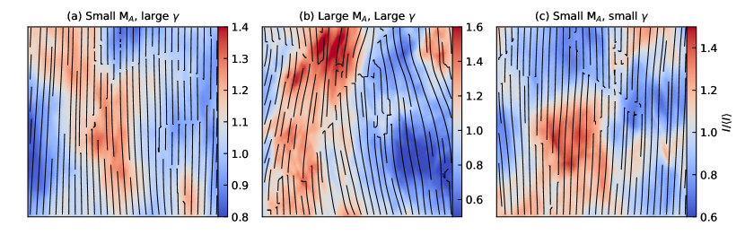
Figure 3: An numerical illustration of the anisotropy in normalized synchrotron intensity map. The black streamlines represent the POS magnetic field orientation. Panel (a): $\langle M_{A}\rangle=0.26$, $\langle M_{s}\rangle=0.66$, and $\langle\gamma\rangle=90^{\circ}$. Panel (b): $\langle M_{A}\rangle=1.21$, $\langle M_{s}\rangle=0.58$, and $\langle\gamma\rangle=90^{\circ}$. Panel (c): $\langle M_{A}\rangle=0.26$, $\langle M_{s}\rangle=0.66$, and $\langle\gamma\rangle=30^{\circ}$.

3.3 Synthetic synchrotron observation

To generate a synthetic spectroscopic cube from our simulations, we utilize the density field, $\rho(\mathbf{x})$, and the magnetic field, $\mathbf{B}(\mathbf{x})$, where $\mathbf{x}=(x,y,z)$ denotes the spatial coordinates. The calculations for synchrotron intensity $I(x,y)$, Stokes parameters $Q(x,y)$ and $U(x,y)$, and the polarization angle $\psi(x,y)$ maps (Getmantsev, 1959; Ginzburg & Syrovatskii, 1969; Rybicki & Lightman, 1979; Lazaryan & Shutenkov, 1990; Waelkens et al., 2009):

$$I(x,y) =\int n_{e}(B_{x}^{2}+B_{y}^{2})B_{\perp}^{\gamma}dz,$$ (5)

$$Q(x,y) =\int-n_{e}(B_{x}^{2}-B_{y}^{2})B_{\perp}^{\gamma}dz,$$ (6)

$$U(x,y) =\int-n_{e}(2B_{x}B_{y})B_{\perp}^{\gamma}dz,$$ (7)

where $B_{\perp}=\sqrt{B_{x}^{2}+B_{y}^{2}}$ represents the magnetic field component perpendicular to the LOS, with $B_{x}$ and $B_{y}$ as its $x$ and $y$ components, respectively. The term $n_{e}=\rho(\mathbf{x})$ signifies the density of relativistic electrons. Considering the synchrotron emission’s relative insensitivity to the electron energy distribution’s spectral index (Lazarian & Pogosyan, 2012; Zhang et al., 2019b), we assume a homogeneous and isotropic electron energy distribution $N(E)dE=N_{0}E^{-p}dE$ with a spectral index $p=3$. This assumption yields a synchrotron emission index of $\gamma=(p-3)/4$. The magnetic field predicted from CNN using $I(x,y)$ is insensitive to Faraday rotation. We therefore did not include the Faraday rotation effect here.

3.4 Training images

Our training input is the synchrotron intensity map $I(x,y)$ generated from the ZEUS-MP/3D simulations, while the AthenaK simulation serves as a validation test. The intensity map is normalized by its maximum intensity so only morphological features in the map are the most important. The $792\times 792$-cells $I(x,y)$ is randomly segmented into $22\times 22$-cell subfields for input into the CNN model. For each subfield, we also generate corresponding projected maps of $\phi^{\rm sub}$, $\gamma^{\rm sub}$, $M_{A}^{\rm sub}$, and $M_{s}^{\rm sub}$ as per the following:

$$\phi^{\rm sub}(x,y) =\arctan(\frac{\int B_{y}(x,y,z)dz}{\int B_{x}(x,y,z)dz}),$$ (8)

$$\gamma^{\rm sub}(x,y) =\arccos(\frac{\int B_{z}(x,y,z)dz}{\int B(x,y,z)dz}),$$

$$M_{A}^{\rm sub} =\frac{v_{\rm inj}^{\rm sub}\sqrt{4\pi\langle\rho\rangle^{\rm sub}}}{\langle B\rangle^{\rm sub}},$$

$$M_{s}^{\rm sub} =\frac{v_{\rm inj}^{\rm sub}}{c_{s}},$$

where $B=\sqrt{B_{x}^{2}+B_{y}^{2}+B_{z}^{2}}$ is the total magnetic field strength, and $B_{x}$, $B_{y}$, and $B_{z}$ are its $x$, $y$, and $z$ components. $\langle\rho\rangle^{\rm sub}$ and $\langle B\rangle^{\rm sub}$ are the mass density and magnetic field strength averaged over the subfield, respectively. $M_{A}^{\rm sub}$ and $M_{s}^{\rm sub}$ are defined using the local velocity dispersion for each subfield (i.e., $v_{\rm inj}^{\rm sub}$), rather than the global turbulent injection velocity $v_{\rm inj}$ used to characterize the full simulation. The ranges of $M_{A}^{\rm sub}$ and $M_{s}^{\rm sub}$ averaged over the subfield in each simulation with different $\gamma$ are listed in Tab. 1, while $\gamma^{\rm sub}$ spans from 0 to 90^∘. These values of $M_{A}^{\rm sub}$, $M_{s}^{\rm sub}$, and $\gamma^{\rm sub}$ cover typical physical conditions of diffuse medium.

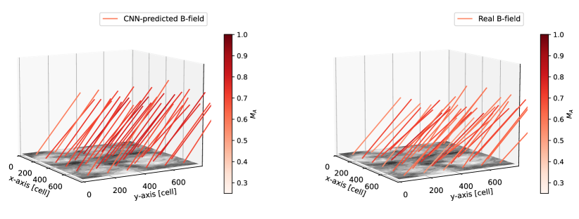
Figure 4: An comparison of the CNN-predicted 3D magnetic fields using the simulation $\langle M_{A}\rangle=0.79$, $\langle M_{s}\rangle=0.61$, and $\langle\gamma\rangle=60^{\circ}$. Each magnetic field segment is constructed by the POS magnetic field’s position angle (i.e., $\phi$) and the inclination angle $\gamma$. Note that the magnetic field obtained is the projection along the LOS and averaged over 132$\times$132 pixels for visualization purposes. The third axis of the LOS is only for 3D visualization purposes and does not provide distance information here. The total intensity map $I$ is placed on the POS, i.e., the $x-y$ plane.

4 Results

4.1 Numerical training and tests

Fig. 3 shows how the Alfvénic Mach number ($M_{A}$) and the inclination angle ($\gamma$) shape the anisotropy within synchrotron intensity maps, particularly focusing on local intensity structures. When both $M_{A}$ and $\gamma$ are small, representing a strong magnetic field and insignificant projection effect, the intensity structures prominently emerge as narrow strips, aligning with the POS magnetic fields. With an increase in $M_{A}$, corresponding to a weakening in the magnetic field, both the magnetic field topology and the synchrotron intensity structures exhibit increased curvature.

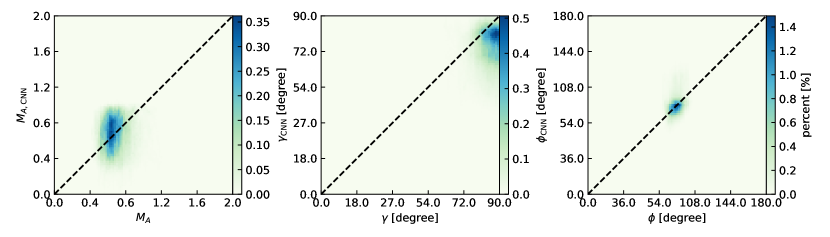
(a) $\langle M_{A}\rangle=0.79$, $\langle M_{s}\rangle=0.61$, $\langle\gamma\rangle=90^{\circ}$

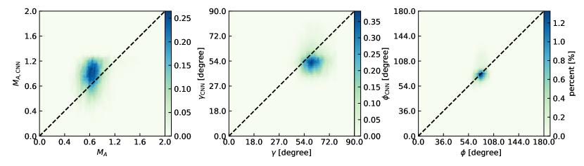
(b) $\langle M_{A}\rangle=0.79$, $\langle M_{s}\rangle=0.61$, $\langle\gamma\rangle=60^{\circ}$

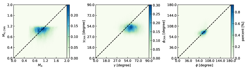
(c) $\langle M_{A}\rangle=1.25$, $\langle M_{s}\rangle=1.21$, $\langle\gamma\rangle=60^{\circ}$

Figure 5: 2D histograms of the CNN-predictions, i.e., $\phi^{\rm CNN}$ (right), $\gamma^{\rm CNN}$ (middle), and $M_{A}^{\rm CNN}$ (left) and the corresponding actual values in simulation. The dashed reference line represents the ideal scenario, where the predicted values and actual values match perfectly.

On the other hand, small $\gamma$ suggests a magnetic field orientation closer to the LOS, diminishing the observed anisotropy due to projection effects. Consequently, the elongation along the POS magnetic field becomes less distinct, indicating a reduced anisotropic degree. Thus, the characteristics of anisotropic elongation, curvature, and degree within the intensity structures offer insights into the magnetic fields’ POS orientation, inclination angle, and magnetization ($M_{A}^{-1}$), respectively.

Fig. 4 offers a visual comparison between the actual 3D magnetic fields from a simulation characterized by $\langle M_{A}\rangle=0.79$, $\langle M_{s}\rangle=0.61$, and $\langle\gamma\rangle=60^{\circ}$, and those predicted by a trained CNN model. In this figure, the orientation of the POS magnetic field, represented by the position angle ($\phi$), and the inclination angle ($\gamma$), are visualized, with the projected $M_{A}$ values depicted through color coding. A significant observation from this comparison is the congruence in the orientations of the actual and CNN-predicted 3D magnetic fields. The predicted $M_{A}$ values, however, are observed to be marginally higher—by approximately 0.1 to 0.2—compared to the actual simulation values.

Fig. 5 presents 2D histograms of the CNN predictions—$\phi^{\rm CNN}$, $\gamma^{\rm CNN}$, and $M_{A}^{\rm CNN}$—against the actual values from two distinct test simulations, Z2 ($\langle M_{A}\rangle=0.79$, $\langle M_{s}\rangle=0.61$) and A0 ($\langle M_{A}\rangle=1.25$, $\langle M_{s}\rangle=1.21$). It is noteworthy that these simulations were generated using different numerical codes: Z2 by ZEUS-MP/3D (Hayes et al., 2006) and A0 by the AthenaK code (Stone et al., 2020). Importantly, simulation A0, characterized by a higher Mach number than those included in the CNN training dataset, was not utilized during the training phase. Despite the inherent differences in the numerical simulations and the turbulence conditions they represent, the histograms reveal a statistical concordance between the CNN predictions and the actual simulation values. The proximity of the data points to the one-to-one reference line indicates a strong agreement between predicted and true values, highlighting the CNN model’s accuracy, albeit with some scatter that reflects deviations from the actual values.

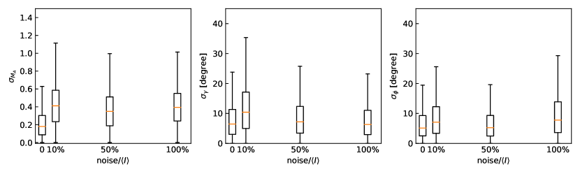
Figure 6: Boxplots of difference in CNN-predicted $\phi^{\rm CNN}$ (right), $\gamma^{\rm CNN}$ (middle), and $M_{A}^{\rm CNN}$ (left) and the actual values in the simulation A0 ($\langle M_{A}\rangle=1.25$, $\langle M_{s}\rangle=1.21$, $\langle\gamma\rangle=60^{\circ}$) with Gaussian noise introduced. The upper and lower black lines represent the deviation’s maximum and minimum, respectively. The box gives ranges of the first (lower) and third quartiles (upper) and the orange line represents the median value. The amplitude of the noise varies from 10%, 50%, to 100% of the mean intensity of the maps, corresponding to signal-to-noise ratios of 10, 2, and 1, respectively.

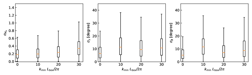
Figure 7: Boxplots of difference in CNN-predicted $\phi^{\rm CNN}$ (right), $\gamma^{\rm CNN}$ (middle), and $M_{A}^{\rm CNN}$ (left) and the actual values in the simulation A0 ($\langle M_{A}\rangle=1.25$, $\langle M_{s}\rangle=1.21$, $\langle\gamma\rangle=60^{\circ}$) when spat. The upper and lower black lines represent the deviation’s maximum and minimum, respectively. The box gives ranges of the first (lower) and third quartiles (upper) and the orange line represents the median value. $k_{\rm min}$ represents the minimum wavenumber remaining in the filtered synchrotron intensity map and $L_{\rm box}$ is the size of simulation box.

4.2 Noise effect

Noise is an inherent challenge in observation that can potentially influence CNN predictions. To evaluate this effect comprehensively, we introduce Gaussian noise into the synchrotron intensity maps used for training the CNN model. The amplitude of this noise varies, representing 10%, 50%, and 100% of the mean intensity of the maps, corresponding to signal-to-noise ratios (SNRs) of 10, 2, and 1, respectively. This allows us to train the CNN model across a range of noise levels.

Fig. 6 presents boxplots that illustrate the deviations between the CNN-predicted values and the actual 3D magnetic field using simulation A0 ($\langle M_{A}\rangle=1.25$, $\langle M_{s}\rangle=1.21$, $\langle\gamma\rangle=60^{\circ}$) as a case study. We quantify these deviations by calculating the absolute differences in the magnetic field’s position angle ($|\phi^{\rm CNN}-\phi|$), inclination angle ($|\gamma^{\rm CNN}-\gamma|$), and Alfvén Mach number ($|M_{A}^{\rm CNN}-M_{A}|$), represented as $\sigma_{\phi}$, $\sigma_{\gamma}$, and $\sigma_{{\rm M}_{A}}$, respectively.

In noise-free conditions, the median values of $\sigma_{M_{A}}$, $\sigma_{\gamma}$, and $\sigma_{\phi}$ are approximately 0.2, 5^∘, and 4^∘. Upon introducing noise to the simulation, uncertainties increase, with the median value of $\sigma_{M_{A}}$ rising to about 0.4, and median $\sigma_{\gamma}$ and $\sigma_{\phi}$ extending to the range of 8^∘ - 10^∘. Remarkably, these uncertainties remain consistent across different SNRs of 10, 2, and 1, underscoring the CNN model’s ability to accurately extract magnetic field information amidst varying levels of noise.

4.3 Removing low-spatial-frequency components

Traditional magnetic field mapping via polarimetry necessitates a comprehensive range of spatial frequencies, incorporating both the high-spatial-frequency data from interferometers and the low-spatial-frequency data from single-dish observations. However, recent studies (Lazarian et al., 2020; Hu & Lazarian, 2022) have illuminated that the anisotropy inherent in MHD turbulence and synchrotron emission is more pronounced at higher spatial frequencies. This revelation suggests that an anisotropy-centric CNN approach could effectively reconstruct the 3D magnetic field morphology using exclusively high-spatial-frequency data. To examine this proposition, we applied a $k$-space filter to synchrotron intensity maps before CNN training, involving: (i) performing a Fast Fourier Transform (FFT) on a 2D map; (ii) filtering out the intensity values at specified wavenumbers $k$ to highlight high-spatial frequencies; and (iii) applying an inverse FFT to transform the filtered map back to the spatial domain.

Fig. 6 presents boxplots showing the deviations—$\sigma_{M_{A}}$, $\sigma_{\gamma}$, and $\sigma_{\phi}$—resulting from the removal of low-spatial-frequency components in the synchrotron intensity maps. Across different scenarios of wavenumber removal ($k<10$, $k<20$, and $k<30$), the median values of $\sigma_{M_{A}}$, $\sigma_{\gamma}$, and $\sigma_{\phi}$ exhibit some variability but generally maintain stability within $<0.4$, $<10^{\circ}$, and $<10^{\circ}$, respectively. This underscores the CNN method’s robustness in probing 3D magnetic fields, even without the contribution of low spatial frequencies—highlighting its particular suitability for processing interferometric data devoid of single-dish measurements.

5 Discussion

5.1 Comparison with earlier studies

Understanding the 3D magnetic field is pivotal for unraveling the complexities of the Galactic Magnetic Field (GMF; Jansson & Farrar 2012) and addressing fundamental questions related to the origins of ultra-high energy cosmic rays (Farrar, 2014; Farrar & Sutherland, 2019), as well as issues concerning Galactic foreground polarization (Kovetz & Kamionkowski, 2015; Planck Collaboration et al., 2016b).

The exploration of 3D magnetic fields within the ISM using CNNs is rapidly progressing. An initiative by Hu et al. (2024a) showcased the use of a CNN model to trace the 3D magnetic field structure in molecular clouds. This achievement was facilitated by CNN’s application to thin velocity channel maps (Lazarian & Pogosyan, 2000; Hu et al., 2023) derived from spectroscopic data.

Building on this CNN approach, our study extends the application of CNN to synchrotron emission, aiming to trace the 3D magnetic field in the warm gas phase. This includes determining the orientation of the POS’s magnetic field, the field’s inclination angle, and the total Alfvén Mach number. As the synchrotron intensity is not subject to Faraday rotation, it does not require multiple frequency measurements to compensate for the Faraday effect. Potential applications of the CNN approach extend across a diverse range of astrophysical environments. These include studying the warm ionized phase of the ISM, the Central Molecular Zone (CMZ), external galaxies, supernova remnants, and galaxy clusters.

5.2 Application to interferometric observations

The challenge of missing low-spatial frequency data in observations made with interferometers, due to constraints imposed by their baseline, is a notable concern in radio astronomy. Instances such as the observations by the Australia Telescope Compact Array (ATCA) at 1.4 GHz (Gaensler et al., 2011), which lacked single-dish measurements, and the Westerbork Synthesis Radio Telescope (WSRT) observations of the 3C 196 field at 350 MHz (Jelić et al., 2015), where single-dish measurements at the same frequency were unfeasible, underscore this issue. Additionally, data from the Low-Frequency Array (LOFAR) also experience the loss of low-spatial frequencies (Jelić et al., 2014).

Notwithstanding these challenges, the absence of low-spatial frequency information does not impede the application of CNNs for probing 3D magnetic fields. This resilience stems from the CNN approach’s foundation on the anisotropy inherent in MHD turbulence and synchrotron radiation, which is more conspicuous at higher spatial frequencies (Lazarian et al., 2020; Hu & Lazarian, 2022). As demonstrated in this study, the CNN model is adept at capturing this anisotropy, leveraging only the high-spatial-frequency data accessible from interferometric observations. This unique capability signifies a significant advantage of the CNN approach, enabling the reconstruction of 3D magnetic fields even in the absence of comprehensive spatial frequency coverage.

5.3 Synergy with other methods

The CNN approach has been applied to spectroscopic observations to trace the 3D magnetic fields (Hu et al., 2024a). Extending CNNs to both spectroscopic and synchrotron emission data enables an in-depth analysis of the distribution and variation of 3D magnetic fields across different ISM phases. Compared to synchrotron emission, training CNNs for conditions in molecular clouds presents additional complexities due to the influence of self-gravity and outflow feedback on fluid dynamics and magnetic field structures (Federrath & Klessen, 2012; Hull & Zhang, 2019; Hu et al., 2022a, b; Vázquez-Semadeni et al., 2024). This necessitates the use of nuanced numerical simulations of molecular clouds for CNN training.

The Synchrotron Intensity Gradient (SIG) technique (Lazarian et al., 2017; Hu et al., 2024b) offers a parallel approach to tracing the POS magnetic field orientation, rooted in the anisotropy of MHD turbulence evident in synchrotron emission. This anisotropy manifests in both sub-Alfvénic and super-Alfvénic turbulence, the latter resulting from the advection of turbulent flows (Hu et al., 2024b). With several numerical and observational validation (Lazarian et al., 2017; Zhang et al., 2019a; Hu et al., 2020, 2024b), SIG serves as a valuable benchmark for assessing the efficacy of CNN-based models, particularly in scenarios where polarization data are scarce, such as radio halos in galaxy clusters.

Furthermore, it should be noted that the inclination angle predicted by the CNN model is inherently limited to the range of [0, 90^∘]. This limitation arises because the anisotropy alone cannot definitively discern whether the magnetic field is oriented towards or away from the observer. A synergy with Faraday rotation measurements (Haverkorn, 2007; Taylor et al., 2009; Oppermann et al., 2012; Xu & Zhang, 2016; Tahani et al., 2019), offers promising avenues to resolve this degeneracy.

6 Summary

In this study, we developed and evaluated a CNN model designed to investigate three-dimensional (3D) magnetic fields, including the orientation of the POS magnetic field, the field’s inclination angle, and total magnetization, utilizing synchrotron intensity maps. Our major findings are summarized as follows:

1. We designed and implemented a CNN model capable of extracting the orientation of the POS magnetic field, the field’s inclination angle, and the overall magnetization from synchrotron intensity maps.

2. Through the utilization of synthetic synchrotron maps for model training, we identified that the median uncertainties for predicting the magnetic field’s position angle ($\phi$) and inclination angle ($\gamma$) remained below $10^{\circ}$, with the Alfvén Mach number ($M_{A}$) uncertainty staying under $0.4$.

3. The model’s robustness against noise was evaluated, demonstrating insensitivity to noise with adequate training, ensuring reliable performance under various observational conditions.

4. Our analyses confirmed the CNN method’s resilience in accurately tracing 3D magnetic fields, even in the absence of low spatial frequencies in the synchrotron images—making it particularly adept for analyzing interferometric data that lacks single-dish measurements.

5. We discussed the potential and future applications of this CNN methodology, particularly its utility in predicting the 3D Galactic Magnetic Fields (GMF), and its implications for comprehending 3D magnetic fields within the Central Molecular Zone (CMZ) and beyond, in external galaxies.

Appendix A Comparison of CNN’s input patch size

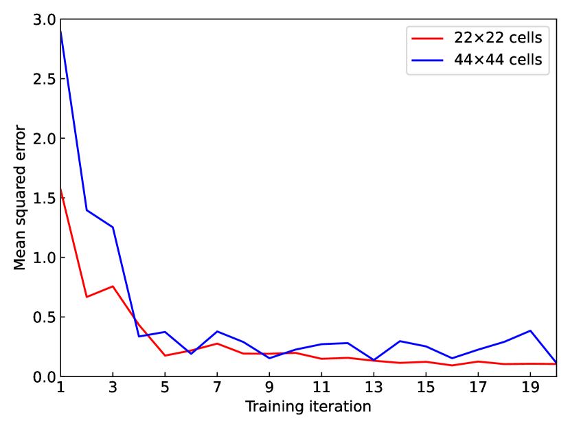
Figure 8: The evolution of CNN’s validation loss, i.e., the mean squared error. Two cases with an input patch size of $22\times 22$ cells or $44\times 44$ cells are tested.

Fig. 8 elucidates the variation in validation loss for two distinct input patch sizes, $22\times 22$ cells and $44\times 44$ cells. The validation loss, representative of the mean squared error between the predicted and actual 3D magnetic fields, is derived from validation datasets comprising patches randomly extracted from the Zeus-series simulations (see Tab. 1). For each training iteration, 100,000 patches are utilized to compute the validation loss, with the loss being averaged across the magnetic field’s POS angle, inclination angle, and Alfvén Mach number. We can see regardless of the input patch size, whether $22\times 22$ or $44\times 44$ cells, the validation loss exhibits a comparable downward trend towards a similar level after an adequate number of training iterations.

References

- Abadi et al. (2015) Abadi, M., Agarwal, A., Barham, P., et al. 2015, TensorFlow: Large-Scale Machine Learning on Heterogeneous Systems. https://www.tensorflow.org/
- Arshakian et al. (2009) Arshakian, T. G., Beck, R., Krause, M., & Sokoloff, D. 2009, A&A, 494, 21, doi: 10.1051/0004-6361:200810964
- Beck (2001) Beck, R. 2001, Space Sci. Rev., 99, 243, doi: 10.1023/A:1013805401252
- Beck (2015) —. 2015, A&A Rev., 24, 4, doi: 10.1007/s00159-015-0084-4
- Bell (1978) Bell, A. R. 1978, MNRAS, 182, 443, doi: 10.1093/mnras/182.3.443
- Bonafede et al. (2014) Bonafede, A., Intema, H. T., Brüggen, M., et al. 2014, ApJ, 785, 1, doi: 10.1088/0004-637X/785/1/1
- Brunetti & Jones (2014) Brunetti, G., & Jones, T. W. 2014, International Journal of Modern Physics D, 23, 1430007, doi: 10.1142/S0218271814300079
- Bykov et al. (2012) Bykov, A. M., Ellison, D. C., & Renaud, M. 2012, Space Sci. Rev., 166, 71, doi: 10.1007/s11214-011-9761-4
- Caprioli & Spitkovsky (2014) Caprioli, D., & Spitkovsky, A. 2014, ApJ, 783, 91, doi: 10.1088/0004-637X/783/2/91
- Chevalier & Luo (1994) Chevalier, R. A., & Luo, D. 1994, ApJ, 421, 225, doi: 10.1086/173640
- Cho & Lazarian (2003) Cho, J., & Lazarian, A. 2003, MNRAS, 345, 325, doi: 10.1046/j.1365-8711.2003.06941.x
- Cho & Vishniac (2000) Cho, J., & Vishniac, E. T. 2000, ApJ, 539, 273, doi: 10.1086/309213
- Condon (1992) Condon, J. J. 1992, ARA&A, 30, 575, doi: 10.1146/annurev.aa.30.090192.003043
- Duan et al. (2021) Duan, D., He, J., Bowen, T. A., et al. 2021, ApJL, 915, L8
- Farrar (2014) Farrar, G. R. 2014, Comptes Rendus Physique, 15, 339, doi: 10.1016/j.crhy.2014.04.002
- Farrar & Sutherland (2019) Farrar, G. R., & Sutherland, M. S. 2019, J. Cosmology Astropart. Phys, 2019, 004, doi: 10.1088/1475-7516/2019/05/004
- Federrath & Klessen (2012) Federrath, C., & Klessen, R. S. 2012, ApJ, 761, 156, doi: 10.1088/0004-637X/761/2/156
- Gaensler et al. (2011) Gaensler, B. M., Haverkorn, M., Burkhart, B., et al. 2011, Nature, 478, 214, doi: 10.1038/nature10446
- Getmantsev (1959) Getmantsev, G. G. 1959, AZh, 36, 422
- Ginzburg & Syrovatskii (1965) Ginzburg, V. L., & Syrovatskii, S. I. 1965, ARA&A, 3, 297, doi: 10.1146/annurev.aa.03.090165.001501
- Ginzburg & Syrovatskii (1969) —. 1969, ARA&A, 7, 375, doi: 10.1146/annurev.aa.07.090169.002111
- Goldreich & Sridhar (1995) Goldreich, P., & Sridhar, S. 1995, ApJ, 438, 763, doi: 10.1086/175121
- Govoni & Feretti (2004) Govoni, F., & Feretti, L. 2004, International Journal of Modern Physics D, 13, 1549, doi: 10.1142/S0218271804005080
- Govoni et al. (2019) Govoni, F., Orrù, E., Bonafede, A., et al. 2019, Science, 364, 981, doi: 10.1126/science.aat7500
- Guan et al. (2021) Guan, Y., Clark, S. E., Hensley, B. S., et al. 2021, ApJ, 920, 6, doi: 10.3847/1538-4357/ac133f
- Haverkorn (2007) Haverkorn, M. 2007, in Astronomical Society of the Pacific Conference Series, Vol. 365, SINS - Small Ionized and Neutral Structures in the Diffuse Interstellar Medium, ed. M. Haverkorn & W. M. Goss, 242. https://arxiv.org/abs/astro-ph/0611090
- Hayes et al. (2006) Hayes, J. C., Norman, M. L., Fiedler, R. A., et al. 2006, ApJS, 165, 188, doi: 10.1086/504594
- Heywood et al. (2022) Heywood, I., Rammala, I., Camilo, F., et al. 2022, ApJ, 925, 165, doi: 10.3847/1538-4357/ac449a
- Hu et al. (2022a) Hu, Y., Federrath, C., Xu, S., & Mathew, S. S. 2022a, MNRAS, 513, 2100, doi: 10.1093/mnras/stac972
- Hu & Lazarian (2022) Hu, Y., & Lazarian, A. 2022, arXiv e-prints, arXiv:2208.06074, doi: 10.48550/arXiv.2208.06074
- Hu et al. (2023) Hu, Y., Lazarian, A., Alina, D., Pogosyan, D., & Ho, K. W. 2023, MNRAS, 524, 2994, doi: 10.1093/mnras/stad1924
- Hu et al. (2022b) Hu, Y., Lazarian, A., Beck, R., & Xu, S. 2022b, ApJ, 941, 92, doi: 10.3847/1538-4357/ac9df0
- Hu et al. (2020) Hu, Y., Lazarian, A., Li, Y., Zhuravleva, I., & Gendron-Marsolais, M.-L. 2020, ApJ, 901, 162, doi: 10.3847/1538-4357/abb1c3
- Hu et al. (2024a) Hu, Y., Lazarian, A., Wu, Y., & Fu, C. 2024a, MNRAS, 527, 11240, doi: 10.1093/mnras/stad3766
- Hu et al. (2021a) Hu, Y., Lazarian, A., & Xu, S. 2021a, ApJ, 915, 67, doi: 10.3847/1538-4357/ac00ab
- Hu et al. (2024b) Hu, Y., Stuardi, C., Lazarian, A., et al. 2024b, Nature Communications, 15, 1006, doi: 10.1038/s41467-024-45164-8
- Hu et al. (2024c) Hu, Y., Xu, S., Arzamasskiy, L., Stone, J. M., & Lazarian, A. 2024c, MNRAS, 527, 3945, doi: 10.1093/mnras/stad3493
- Hu et al. (2021b) Hu, Y., Xu, S., & Lazarian, A. 2021b, ApJ, 911, 37, doi: 10.3847/1538-4357/abea18
- Hull & Zhang (2019) Hull, C. L. H., & Zhang, Q. 2019, Frontiers in Astronomy and Space Sciences, 6, 3, doi: 10.3389/fspas.2019.00003
- Jansson & Farrar (2012) Jansson, R., & Farrar, G. R. 2012, ApJ, 761, L11, doi: 10.1088/2041-8205/761/1/L11
- Jelić et al. (2014) Jelić, V., de Bruyn, A. G., Mevius, M., et al. 2014, A&A, 568, A101, doi: 10.1051/0004-6361/201423998
- Jelić et al. (2015) Jelić, V., de Bruyn, A. G., Pandey, V. N., et al. 2015, A&A, 583, A137, doi: 10.1051/0004-6361/201526638
- Jokipii (1966) Jokipii, J. R. 1966, ApJ, 146, 480, doi: 10.1086/148912
- Kovetz & Kamionkowski (2015) Kovetz, E. D., & Kamionkowski, M. 2015, Phys. Rev. D, 91, 081303, doi: 10.1103/PhysRevD.91.081303
- Kowal & Lazarian (2010) Kowal, G., & Lazarian, A. 2010, ApJ, 720, 742, doi: 10.1088/0004-637X/720/1/742
- Larochelle et al. (2007) Larochelle, H., Erhan, D., Courville, A., Bergstra, J., & Bengio, Y. 2007, in Proceedings of the 24th International Conference on Machine Learning, ICML ’07 (New York, NY, USA: Association for Computing Machinery), 473–480, doi: 10.1145/1273496.1273556
- Lazarian (2006) Lazarian, A. 2006, ApJ, 645, L25, doi: 10.1086/505796
- Lazarian & Pogosyan (2000) Lazarian, A., & Pogosyan, D. 2000, ApJ, 537, 720, doi: 10.1086/309040
- Lazarian & Pogosyan (2012) —. 2012, ApJ, 747, 5, doi: 10.1088/0004-637X/747/1/5