Tensor Neural Network Interpolation and Its Applications

Abstract

Based on tensor neural network, we propose an interpolation method for high dimensional non-tensor-product-type functions. This interpolation scheme is designed by using the tensor neural network based machine learning method. This means that we use a tensor neural network to approximate high dimensional functions which has no tensor product structure. In some sense, the non-tenor-product-type high dimensional function is transformed to the tensor neural network which has tensor product structure. It is well known that the tensor product structure can bring the possibility to design highly accurate and efficient numerical methods for dealing with high dimensional functions. In this paper, we will concentrate on computing the high dimensional integrations and solving high dimensional partial differential equations. The corresponding numerical methods and numerical examples will be provided to validate the proposed tensor neural network interpolation.

Keywords. Tensor neural network, interpolation, machine learning, high dimensional integration, high dimensional equations.

AMS subject classifications. 65N30, 65N25, 65L15, 65B99.

1 Introduction

There exist many high-dimensional problems such as quantum mechanics, statistical mechanics, and financial engineering in modern sciences and engineering. Traditional numerical methods like finite difference, finite element, and spectral methods are typically confined to solving low-dimensional problems. However, applying these classical methods to high-dimensional problems will encounter the so-called “curse of dimensionality”.

Due to its universal approximation property, the fully connected neural network (FNN) is the most widely used architecture to build the functions for solving high-dimensional PDEs. There are several types of well-known FNN-based methods such as deep Ritz [1], deep Galerkin method [8], PINN [7], and weak adversarial networks [14] for solving high-dimensional PDEs by designing different loss functions. Among these methods, the loss functions always include computing high-dimensional integrations for the functions defined by FNN. For example, the loss functions of the deep Ritz method, deep Galerkin method and weak adversarial networks method require computing the integrations on the high-dimensional domain for the functions constructed by FNN. Direct numerical integration for the high-dimensional functions also meets the “curse of dimensionality”. Always, the high-dimensional integration is computed using the Monte-Carlo method along with some sampling tricks [1, 3]. Due to the low convergence rate of the Monte-Carlo method, the solutions obtained by the FNN-based numerical methods are challenging to achieve high accuracy and stable convergence process. This means that the Monte-Carlo method decreases computational work in each forward propagation while decreasing the simulation accuracy, efficiency and stability of the FNN-based numerical methods for solving high-dimensional PDEs.

Recently, we propose a type of tensor neural network (TNN) and the corresponding machine learning method to solve high-dimensional problems with high accuracy. The most important property of TNN is that the corresponding high-dimensional functions can be easily integrated with high accuracy and high efficiency. Then the deduced machine learning method can arrive high accuracy for solving high-dimensional problems. The reason is that the high dimensional integration of TNN in the loss functions can be transformed into one-dimensional integrations which can be computed by the classical quadrature schemes with high accuracy. The TNN based machine learning method has already been used to solve high-dimensional eigenvalue problems and boundary value problems based on the Ritz type of loss functions [9]. Furthermore, in [12], the multi-eigenpairs can also been computed with machine learning method which is designed by combining the TNN and Rayleigh-Ritz process. Furthermore, with the help of TNN, the a posteriori error estimator can be adopted as the loss function of the machine learning method for solving high dimensional boundary value problems and eigenvalue problems [10]. So far, the TNN based machine learning method has shown good ability for solving high dimensional problems which having only tensor product coefficients and source terms. The aim and main contribution of this paper is to design a type of TNN based interpolation method for the non-tensor-product-type functions. Then using this interpolation method to approximate the non-tensor-product coefficients and then modify the non-tensor-product-type problems to the corresponding tensor product one. Then the TNN based machine learning method can be adopted to solve the deduced tensor product problems with high accuracy.

An outline of the paper goes as follows. In Section 2, we investigate the dependence of the accuracy for machine learning methods on the accuracy of integration through a numerical experiment. Section 3 is devoted to introducing the TNN structure and the corresponding approximation property. In Section 4, the TNN based interpolation will be proposed to approximate high-dimensional functions. In Section 5, we introduce the way to compute the high dimensional integrations of non-tensor-product-type functions by using TNN interpolation. Section 6 is devoted to introducing the application of TNN interpolation to solving high dimensional partial differential equations with non-tensor-product-type coefficients and source terms. Section 7 gives some numerical examples to validate the accuracy and efficiency of the proposed TNN based machine learning method. Some concluding remarks are given in the last section.

2 Integration accuracy and machine learning accuracy

As mentioned above, the loss functions in common machine learning methods for solving PDEs always include high dimensional integrations for the functions defined by neural networks. In this section, we investigate the dependence of the accuracy of machine learning method on the integration accuracy. The aim here is to explore the importance of the integration accuracy for the machine learning method.

We do the numerical investigations of the machine learning accuracy for the Deep Ritz and PINN methods with different integration schemes. To be specific, we consider the following eigenvalue problems: Find $(\lambda,u)\in\mathbb{R}\times H_{0}^{1}(\Omega)$ such that

$$\left\{\begin{aligned} -\Delta u&=\lambda u,\ \ \ &x\in&\Omega,\\ u&=0,\ \ \ &x\in&\partial\Omega,\end{aligned}\right.$$

where $\Omega:=[0,1]^{2}$. We consider this two dimensional problem so that computing the integrations included in the loss function using classical Gauss quadrature scheme becomes feasible. Let $\phi(x;\theta)$ denote the neural network. Here, we check and compare the numerical performances of the following four strategies:

1. (RitzMC): Use the Deep Ritz method with the following loss function

   $$\mathcal{L}_{\rm DRM}(x;\theta)=\frac{\int_{\Omega}|\nabla\phi(x;\theta)|^{2}dx}{\int_{\Omega}|\phi(x;\theta)|^{2}dx}$$ (2.1)

   and compute the included two dimensional integrations with Monte Carlo integration method.

2. (RitzGauss): Use the Deep Ritz method with loss function (2.1) and compute the included two dimensional integrations with Gauss quadrature method.

3. (PINNMC): Use the following loss function based on the idea of PINN method and Deep Galerkin method

   $$\mathcal{L}_{\rm PINN}(x;\theta) = \|\Delta\phi(x;\theta)+\lambda(x;\theta)\phi(x;\theta)\|_{L^{2}(\Omega)}^{2}$$ (2.2)

   $$= \left\|\Delta\phi(x;\theta)+\frac{\int_{\Omega}|\nabla\phi(x;\theta)|^{2}dx}{\int_{\Omega}|\phi(x;\theta)|^{2}dx}\phi(x;\theta)\right\|_{L^{2}(\Omega)}^{2}.$$

   and compute the two dimensional integrations with Monte Carlo integration method.

4. (PINNGauss): Use the loss function (2.2) and compute the two dimensional integration with Gauss quadrature method.

To guarantee the fairness of the numerical comparison, we use the same neural network structures in all four experiments. The fully connected neural network with three hidden layers, with each layer having 50 neurons, is adopted here. The sine function is chosen as the activation function. In order to guarantee the homogeneous boundary condition, we multiply $\phi(x;\theta)$ by $x_{1}(1-x_{1})x_{2}(1-x_{2})$, and still denote the resulting function as $\phi(x;\theta)$ for notational convenience. The same number of quadrature points is used to compute the two dimensional integrations included in the loss functions. Specifically, for Gauss quadrature method, we decompose the interval $[0,1]$ into $20$ subintervals and choose $8$ Gauss quadrature points in each subinterval to obtain the composite quadrature points set $X$ of one dimension. Then, we generate the two dimensional quadrature points using the Cartesian product of $X$ and itself, i.e., $X\times X$, which contains $25,600$ two dimensional quadrature points in total. As for the Monte Carlo integration method, we sample 25,600 uniformly distributed points in $[0,1]^{2}$ in each iteration step. The Adam optimizer with learning rate 0.0003 is adopted for 500,000 iteration steps in all four experiments.

We record the network model, and compute the relative error

$$e_{\lambda}:=\frac{|\lambda-\lambda^{*}|}{\lambda^{*}}$$

of the corresponding approximate eigenvalue $\lambda$ for the exact eigenvalue $\lambda^{*}$ after each $100$ steps. Figure 1 shows the relative errors of four methods during the training process.

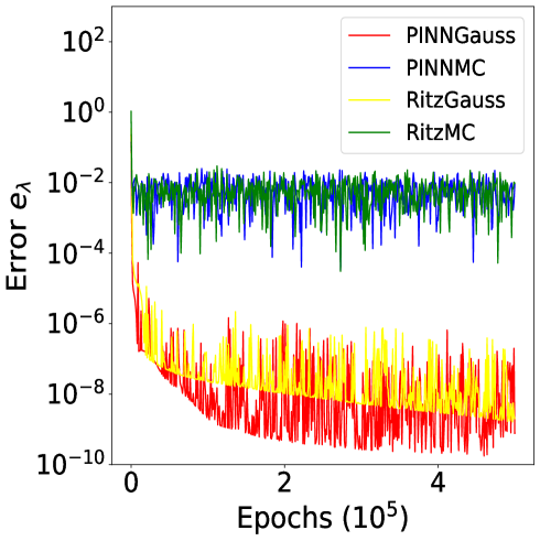
Figure 1: Relative errors of four methods during the training process.

It can be easily observed that the performances of two different loss functions (2.1) and (2.2) are similar, while what really matters is the choice of the numerical integration method. To be specific, with the high-accuracy Gauss quadrature method, the RitzGauss and PINNGauss methods are able to achieve obviously higher accuracy than that of the RitzMC and PINNMC methods.

The results above give a hint that the accuracy of computing the integrations included in the loss functions indeed plays a significant role for the accuracy of the machine learning methods for solving PDEs. And therefore, it’s necessary for the machine learning methods to guarantee the computation accuracy, such as the integration accuracy during the iteration process. Notice that we consider the two dimensional problem in this section since the two dimensional Gauss quadrature method can be leveraged in this case. However, in high dimensional cases, using Gauss quadrature method to guarantee the integration accuracy is not realistic and feasible due to the curse of dimensionality. And this motivates us to design the tensor neural network structure and TNN based machine learning methods [9, 10, 11], which assure the high dimensional integration accuracy within acceptable computational complexity, and therefore achieve high accuracy in solving high dimensional PDEs.

3 Tensor neural network architecture

In this section, we introduce the architecture of TNN and its approximation property which have been discussed and investigated in [9]. The TNN is a neural network of low-rank structure, which is built by the tensor product of several one-dimensional input and multi-dimensional output subnetworks. Due to the low-rank structure of TNN, an efficient and accurate quadrature scheme can be designed for the TNN-related high-dimensional integrations such as the inner product of two TNNs. In [9], we introduce TNN in detail and propose its numerical integration scheme with the polynomial scale computational complexity of the dimension. For each $i=1,2,\cdots,d$, we use $\Phi_{i}(x_{i};\theta_{i})=(\phi_{i,1}(x_{i};\theta_{i}),\phi_{i,2}(x_{i};\theta_{i}),\cdots,\phi_{i,p}(x_{i};\theta_{i}))$ to denote a subnetwork that maps a set $\Omega_{i}\subset\mathbb{R}$ to $\mathbb{R}^{p}$, where $\Omega_{i},i=1,\cdots,d,$ can be a bounded interval $(a_{i},b_{i})$, the whole line $(-\infty,+\infty)$ or the half line $(a_{i},+\infty)$. The number of layers and neurons in each layer, the selections of activation functions and other hyperparameters can be different in different subnetworks. In this paper, in order to improve the numerical stability further, the TNN is defined as follows:

$$\Psi(x;\Theta)=\sum_{j=1}^{p}c_{j}\widehat{\phi}_{1,j}(x_{1};\theta_{1})\widehat{\phi}_{2,j}(x_{2};\theta_{2})\cdots\widehat{\phi}_{d,j}(x_{d};\theta_{d})=\sum_{j=1}^{p}c_{j}\prod_{i=1}^{d}\widehat{\phi}_{i,j}(x_{i};\theta_{i}),$$ (3.1)

where $c=\{c_{j}\}_{j=1}^{p}$ is a set of trainable parameters, $\Theta=\{c,\theta_{1},\cdots,\theta_{d}\}$ denotes all parameters of the whole architecture. For $i=1,\cdots,d,j=1,\cdots,p$, $\widehat{\phi}_{i,j}(x_{i},\theta_{i})$ is a normalized functions as follows:

$$\widehat{\phi}_{i,j}(x_{i},\theta_{i})=\frac{\phi_{i,j}(x_{i},\theta_{i})}{\|\phi_{i,j}(x_{i},\theta_{i})\|_{L^{2}(\Omega_{i})}}.$$ (3.2)

The TNN architecture (3.1) and the one defined in [9] are mathematically equivalent, but (3.1) has better numerical stability during the training process. Figure 2 shows the corresponding architecture of TNN. From Figure 2 and numerical tests, we can find the parameters for each rank of TNN are correlated by the FNN, which guarantee the stability of the TNN-based machine learning methods. This is also an important difference from the tensor finite element methods.

Figure 2: Architecture of TNN. Black arrows mean linear transformation (or affine transformation). Each ending node of blue arrows is obtained by taking the scalar multiplication of all starting nodes of blue arrows that end in this ending node. The final output of TNN is derived from the summation of all starting nodes of red arrows.

In [9] we introduce and prove the following approximation result to the functions in the space $H^{m}(\Omega_{1}\times\cdots\times\Omega_{d})$ under the sense of $H^{m}$-norm.

Theorem 3.1.

Assume that each $\Omega_{i}$ is an interval in $\mathbb{R}$ for $i=1,\cdots,d$, $\Omega=\Omega_{1}\times\cdots\times\Omega_{d}$, and the function $f(x)\in H^{m}(\Omega)$. Then for any tolerance $\varepsilon>0$, there exist a positive integer $p$ and the corresponding TNN defined by (3.1) such that the following approximation property holds

$$\|f(x)-\Psi(x;\theta)\|_{H^{m}(\Omega)}<\varepsilon.$$ (3.3)

The TNN seems rather simple, but it actually has a surprising rich structure. The motivation for employing the TNN architectures is to provide high accuracy and high efficiency in calculating variational forms of high-dimensional problems in which high-dimensional integrations are included. The TNN itself can approximate functions in Sobolev space with respect to $H^{m}$-norm. For more information about the rank estimates, please refer to [9]. The major contribution of this paper is to propose a TNN-based interpolation method, to approximate high dimensional functions. Its applications for computing high dimensional integrations and solving high dimensional partial differential equations also shows the advantages of TNN.

4 Tensor neural network interpolation

In this section, we introduce the tensor neural network interpolation method for the desired function $f(x)$. In this article, we say that a function $g(x)$ is of tensor product type, or is a tensor-product-type function, if $g(x)$ can be expressed in the form of

$$g(x)=\sum_{j=1}^{p}g_{1,j}(x_{1})g_{2,j}(x_{2})\cdots g_{d,j}(x_{d})=\sum_{j=1}^{p}\prod_{i=1}^{d}g_{i,j}(x_{i})$$ (4.1)

for some one-dimensional functions $g_{i,j}(x_{i})$. Recall that TNN function $\Psi(x;\Theta)$ defined by (3.1) is of tensor product type with $\widehat{\phi}_{i,j}(x_{i};\theta_{i})$ being one-dimensional-input neural network. In the previous section, we demonstrate the importance of integration accuracy on the accuracy of machine learning method for solving PDEs. When the dimension of the problem is high, computing the high dimensional integration within a satisfactory accuracy under limited computing resources is difficult, unless the integrated function possesses some desirable properties. In [9], the efficient and accurate integration scheme for a function of tensor product type is designed. The core idea is to transform the high dimensional integration into the product of one dimensional one, and use classical numerical integration scheme such as Gauss quadrature scheme to compute these one dimensional integration. However, in practice, we also encounter some scenarios where the integrated function is not of tensor product type. For example, when we use machine learning method to solve some high dimensional problems with non-tensor-product-type coefficients or source terms, the computation of the loss function is always tricky.

The aim of the interpolation is to find a tensor neural network $\Psi(x,\theta)$ to approximate the integrated function $f(x)$ (possibly non-tensor-product-type) in some sense so that we can use the approximated function to compute the high dimensional integration of $f(x)$. Note that finding an approximation for high dimensional functions is generally not easier than computing the integrations of these high dimensional functions. However, in machine learning method for PDEs, there requires lots of high dimensional integrations computation. Then finding an approximated function that can be integrated with high efficiency and accuracy can improve the accuracy of machine learning method and speed up the learning process, since we only do the TNN interpolation once and use the approximate function to replace the original one during the whole training process. Therefore, the interpolation trick is of great importance for TNN based machine learning methods to be applied again in the case of non-tensor-product-type coefficients or source terms, due to the tensor product structure of the TNN approximation function.

It is a common idea to use an easy-to-integrated function to approximate the integrated function. For example, in one dimensional integration, classical quadrature schemes are designed by using polynomial interpolation for the integrated functions. Especially, the idea behind the well known Gauss quadrature schemes are based on the special choice of the interpolation points. In this paper, we use TNN to approximate the integrated function due to its universal approximation ability and the fact that TNN function can be integrated in an efficient and accurate way [9].

The machine learning method is adopted to finish this approximating task. To be specific, at each iteration $\ell$, we obtain a bunch of training points $x_{k}^{(\ell)}:=(x_{k,1}^{(\ell)},\cdots,x_{k,d}^{(\ell)})^{\top}$, $k=1,\cdots,K$ according to some sampling rules, and minimize the squared loss

$$L_{\ell}(\Theta):= \sum_{k=1}^{K}\left(\Psi(x_{k}^{(\ell)},\Theta)-f(x_{k}^{(\ell)})\right)^{2}$$ (4.2)

$$= \sum_{k=1}^{K}\left(\sum_{j=1}^{p}c_{j}\prod_{i=1}^{d}\widehat{\phi}_{i,j}(x_{k,i}^{(\ell)};\theta_{i})-f(x_{k}^{(\ell)})\right)^{2},$$

to obtain the desired network parameters $\Theta=\{c,\theta_{1},\cdots,\theta_{d}\}$. This procedure is repeated $M$ times until we obtain good enough results on the validation scheme, such as the accuracy on the test points set.

In the optimization process, we split the parameters into two groups $\{c\}$ and $\{\theta_{1},\cdots,\theta_{d}\}$. The parameter $c$ can be regarded as the linear coefficients on the $p$-dimensional subspace $V_{p}^{(t)}:=\text{span}\left\{\varphi_{j}(x;\theta^{(t)}):=\prod_{i=1}^{d}\widehat{\phi}_{i,j}\left(x_{i};\theta_{i}^{(t)}\right)\right\}$. And therefore, we only need to solve a linear equation to obtain the optimal coefficient $c$ on the current subspace $V_{p}^{(t)}$ in the sense of the squared loss on training points. Using the optimal coefficient $c$, we update the network parameters $\{\theta_{j}\}$ by minimizing the loss function with some optimization algorithm. The TNN interpolation method to obtain an approximation for a given target function is defined in Algorithm 1.

Input: Target function $f(x)$, TNN function $\Psi(x;\Theta)$ defined by (3.1), initial model parameters $\Theta$, domain $\Omega$.

Output: Learned approximate TNN function $\Psi(x;\Theta^{*})$

Hyper-parameters : Number of total training iterations $M$, number of training points in each iteration $K$, number of optimization steps $N$ for each training points set, hyperparameters of optimization algorithm such as step size $\gamma$.

1 for $\ell\leftarrow 1$ to $M$ do

2      Sample $x_{k}^{(\ell)}\in\Omega$, $k=1,\dots,K$ according to some sampling rules

3      for $t\leftarrow 1$ to $N$ do

4           Assemble matrix $A^{(t)}$ and vector $B^{(t)}$, where the entries are defined as follows

$$A_{m,n}^{(t)} =\sum_{k=1}^{K}\prod_{i=1}^{d}\widehat{\phi}_{i,m}(x_{k,i}^{(\ell)};\theta_{i}^{(t-1)})\prod_{i=1}^{d}\widehat{\phi}_{i,n}(x_{k,i}^{(\ell)};\theta_{i}^{(t-1)}),\ 1\leq m,n\leq p,$$

$$B_{m}^{(t)} =\sum_{k=1}^{K}f(x_{k}^{(\ell)})\prod_{i=1}^{d}\widehat{\phi}_{i,m}(x_{k,i}^{(\ell)};\theta_{i}^{(t-1)}),\ 1\leq m\leq p.$$

5          Solve the following linear equation to obtain the solution $c\in\mathbb{R}^{p}$:

$$A^{(t)}c=B^{(t)},$$

and update the coefficient parameter as $c^{(t)}=c$.

6          Compute the loss function

$$\mathcal{L}_{\ell}^{(t)}(\theta^{(t-1)})=\sum_{k=1}^{K}\left(\sum_{j=1}^{p}c_{j}^{(t)}\prod_{i=1}^{d}\widehat{\phi}_{i,j}\left(x_{k,i}^{(\ell)};\theta_{i}^{(t-1)}\right)-f(x_{k}^{(\ell)})\right)^{2}.$$

7          Use an optimization step to update the neural network parameters of TNN as follows:

$$\theta^{(t)}=\theta^{(t-1)}-\gamma\frac{\partial\mathcal{L}_{\ell}^{(t)}}{\partial\theta}(c^{(t)},\theta^{(t-1)}).$$

8           end for

9          

10           end for

Algorithm 1 TNN interpolation method

For different target function $f(x)$ and computing domain $\Omega$, we can literally design all the details as we need, including the parameters, the validation scheme and so on. Recall that our primary motivation is to obtain an optimal function, which can be integrated with high efficiency and accuracy, to replace the non-tensor-product coefficient in the PDEs and then use the TNN based machine learning method to solve the concerned PDEs. Therefore all the interpolation work can be done off-line, and we can repeat the procedure until we obtain an satisfactory appropriate function as we need.

5 TNN interpolation for high dimensional integration

In this section, based on the TNN interpolation, we design a type of machine learning method for computing high dimensional integrations. As an example, we are concerned with the following high dimensional integration for the $f(x)$ on $\Omega\subset\mathbb{R}^{d}$

$$I=\int_{\Omega}f(x)dx.$$ (5.1)

Actually, the process is direct and simple. First, we produce the TNN interpolation $\Psi(x,\theta)$ to approximate the target function $f(x)$ based on the machine learning process defined by Algorithm 1. Then, with the help of TNN interpolation $\Psi(x,\theta)$, we can compute the following integration as an approximation to the high dimensional integration (5.1)

$$I\approx\int_{\Omega}\Psi(x,\theta)dx.$$ (5.2)

The method here can be extended to compute the numerical integrations of polynomial composite functions of TNN and their derivatives. For more information about computing high dimensional integrations of TNN functions, please refer to [9]. For example, the method here can be used to compute the following integrations

$$\int_{\Omega}|f|^{2}dx,\ \ \ \int_{\Omega}|\nabla f|^{2}dx,\ \ \ \int_{\Omega}|-\Delta f|^{2}dx.$$ (5.3)

About the way and complexity for computing numerical integrations of polynomial composite functions of TNN and their derivatives, please refer to [9]. For example, we have the following way to compute $\int_{\Omega}\Psi dx$ and $\int_{\Omega}|\Psi|^{2}dx$

$$\int_{\Omega}\Psi(x,\theta)dx = \sum_{j=1}^{p}\prod_{i=1}^{d}\int_{\Omega_{i}}\phi_{i,j}(x_{i},\theta_{i})dx_{i}\approx\sum_{j=1}^{p}\prod_{i=1}^{d}\left(\sum_{n_{i}=1}^{N_{i}}w_{i}^{(n_{i})}\phi_{i,j}(x_{i}^{(n_{i})})\right),$$

$$\int_{\Omega}|\Psi|^{2}dx = \sum_{j=1}^{p}\sum_{k=1}^{p}\prod_{i=1}^{d}\left(\int_{\Omega_{i}}\phi_{i,j}(x_{i})\phi_{i,k}(x_{i})dx_{i}\right)$$

$$\approx \sum_{j=1}^{p}\sum_{k=1}^{p}\prod_{i=1}^{d}\left(\sum_{n_{i}=1}^{N_{i}}w_{i}^{(n_{i})}\phi_{i,j}(x_{i}^{(n_{i})})\phi_{i,k}(x_{i}^{(n_{i})})\right),$$

where $\Omega=\Omega_{1}\times\Omega_{d}$, $(x_{i}^{(n_{i})},w_{i}^{(n_{i})})$ denotes the quadrature points and weights on the domain $\Omega_{i}$, $n_{i}=1,\cdots,N_{i}$.

The method here give a new view to understand the numerical interpolation and numerical integration. Different from Monte-Carlo based schemes, it give another way to compute the high dimensional numerical integrations. More about this topic, please refer to [2, 4, 6, 13].

6 TNN interpolation for solving high dimensional PDEs

In this section, we introduce the application of TNN interpolation method for solving high dimensional elliptic problem with non-tensor-product-type coefficients and source term. The numerical scheme here is designed based on the combination of the TNN interpolation method and TNN-based machine learning method [10]. We assume the physical domain $D=D_{1}\times\cdots\times D_{d}$ with $D_{i}=[a_{i},b_{i}]$ for $i=1,\cdots,d$. It is noted that the tensor product structure plays an important role in reducing the dependence on dimensions in numerical integration. We will find that the high accuracy of the high-dimensional integrations of TNN functions leads to the corresponding machine learning method has high accuracy for solving the high-dimensional parametric elliptic equations.

As an example, we consider the following second order elliptic problem: Find $\bar{u}\in H_{0}^{1}(\Omega)$ such that

$$\left\{\begin{array}[]{rcl}-{\rm div}(a(x)\nabla\bar{u})+b(x)\bar{u}&=&f(x),\ \ \ \ {\rm in}\ \Omega,\\ \bar{u}&=&0,\ \ \quad\quad{\rm on}\ \partial\Omega,\end{array}\right.$$ (6.3)

where the coefficients $a(x)\geq a_{\min}>0$ and $b(x)\geq 0$, the source term $f\in L^{2}(\Omega)$ may be non-tensor-product-type functions.

First, we use the TNN interpolation method defined in Algorithm 1 to get the tensor neural network functions $\widehat{a}(x)$, $\widehat{b}(x)$ and $\widehat{f}(x)$, respectively. Then the concerned equation (6.3) can be modified to the following approximate one: Find $u\in H_{0}^{1}(\Omega)$ such that

$$\left\{\begin{array}[]{rcl}-{\rm div}(\widehat{a}(x)\nabla u)+\widehat{b}(x)u&=&\widehat{f}(x),\ \ \ \ {\rm in}\ \Omega,\\ u&=&0,\ \ \ \ {\rm on}\ \partial\Omega.\end{array}\right.$$ (6.6)

The solution $u$ here can be regarded as the approximation to the exact solution $\bar{u}$ of the equation (6.3).

For designing the TNN based machine learning method, we build the following TNN function

$$\Psi(x)=\sum\limits_{j=1}^{p}c_{j}\prod_{i=1}^{d}\widehat{\phi}_{i,j}(x_{i}),$$ (6.7)

where $x=[x_{1},\cdots,x_{d}]^{\top}$. In order to deal with the boundary condition, following [9], for $i=1,\cdots,d$, the $i$-th subnetwork $\psi_{i}(x_{i};\theta_{i})$ is defined as follows:

$$\phi_{i}(x_{i}) := (x_{i}-a_{i})(b_{i}-x_{i})\widehat{\phi}_{i}(x_{i})$$

$$= \big{(}(x_{i}-a_{i})(b_{i}-x_{i})\widehat{\phi}_{i,1}(x_{i}),\cdots,(x_{i}-a_{i})(b_{i}-x_{i})\widehat{\phi}_{i,p}(x_{i})\big{)}^{\top},$$

where $\widehat{\phi}_{i}(x_{i};\theta_{i})$ is an FNN from $\mathbb{R}$ to $\mathbb{R}^{p}$ with sufficiently smooth activation functions, such that $\Psi(x)\in H_{0}^{1}(\Omega)$.

Theorem 6.1.

If $\bar{u}$ and $u$ are solutions of (6.3) and (6.6), respectively. Assume the coefficients $a$ and $\widehat{a}$ has the same lower bound $a_{\min}$, both $b$ and $\widehat{b}$ are positive. Then

$$\|\bar{u}-u\|_{V}\leq\left(\|f-\widehat{f}\|_{-1}+\left(\|a-\widehat{a}\|_{L^{\infty}(\Omega)}+\|b-\widehat{b}\|_{L^{\infty}(\Omega)}\right)\|f\|_{-1}\right),$$ (6.8)

where $V:=H_{0}^{1}(\Omega)$ and the energy norm $\|\cdot\|_{V}$ is defined as follows

$$\|v\|_{V}:=\sqrt{(\widehat{a}\nabla v,\nabla v)+(\widehat{b}v,v)},\ \ \ \forall v\in V.$$

Proof.

The variational form for the equation (6.3) can be defined as follows

$$(a\nabla\bar{u},\nabla v)+(b\bar{u},v)=(f,v),\ \ \ \forall v\in V.$$ (6.9)

Similarly, the weak form for the modified problem (6.6) can be given as follows

$$(\widehat{a}\nabla u,\nabla v)+(\widehat{b}u,v)=(\widehat{f},v),\ \ \ \forall v\in V.$$ (6.10)

From (6.9), (6.10) and the regularity $\|u\|_{1}\leq C\|f\|_{-1}$, we have following estimates

$$(\widehat{a}\nabla(\bar{u}-u),\nabla v)+(\widehat{b}(\bar{u}-u),v)=(f-\widehat{f},v)+((\widehat{a}-a)\nabla u,\nabla v)+((\widehat{b}-b)u,v)$$

$$\leq\left(\|f-\widehat{f}\|_{-1}+\|a-\widehat{a}\|_{L^{\infty}(\Omega)}\|u\|_{1}+\|b-\widehat{b}\|_{L^{\infty}(\Omega)}\|u\|_{0}\right)\|v\|_{1}$$

$$\leq C\left(\|f-\widehat{f}\|_{-1}+\left(\|a-\widehat{a}\|_{L^{\infty}(\Omega)}+\|b-\widehat{b}\|_{L^{\infty}(\Omega)}\right)\|f\|_{-1}\right)\|v\|_{1},\ \ \ \forall v\in V.$$ (6.11)

Setting $v=\bar{u}-u$ in (6) leads to the following inequality

$$\|\bar{u}-u\|_{V}\leq C\left(\|f-\widehat{f}\|_{-1}+\left(\|a-\widehat{a}\|_{L^{\infty}(\Omega)}+\|b-\widehat{b}\|_{L^{\infty}(\Omega)}\right)\|f\|_{-1}\right).$$

This is the desired result (6.8) and the proof is complete. ∎

Theorem 6.1 shows that the way in this section is reasonable for solving partial differential equations with the coefficients being interpolated by the TNN functions. The detailed computing process can be decomposed into two steps. In the first step, we use TNN based machine learning method by Algorithm 1 to interpolate the non-tensor-product-type coefficients or source term of the concerned problem (6.3). In the second step, the TNN based machine learning method [10] is adopted to solve the modified problem (6.6).

7 Numerical examples

In this section, we provide two numerical examples to validate the TNN interpolation method which is defined by Algorithm 1. In order to check the validation, the TNN interpolation method is used to compute the integrations of (possibly non-tensor-product-type) high dimensional functions and solve the high dimensional partial differential equations with non-tensor-product type of coefficients and source term.

7.1 High dimensional integration

In this subsection, we check the numerical performance of the TNN interpolation for the high dimensional integrations. For this aim, we set the desired function $f(x)=\exp\left(\sum_{i=1}^{8}x_{i}^{2}\right)$ on the domain $\Omega=[0,1]^{8}$. The reason to choose a tensor-product-type function $f(x)$ is that we can compute the integration error accurately.

We execute the interpolation process following Algorithm 1. In each iteration, we uniformly sample $8000$ points in domain $[0,1]^{8}$. As for network structure, we choose the rank $p=50$, and each subnetwork of TNN is chosen as the FNN with two hidden layers and each hidden layer has 50 neurons. The sine function is chosen as the activation function. We conduct the optimization process using the Adam optimizer with learning rate 0.003 in the first 50,000 steps and then the LBFGS optimizer with learning rate 0.1 in the subsequent 200 steps. We repeat the iterations for 20 times to obtain the final approximate function. In order to validate the accuracy of the integration using TNN interpolation method, the interval $[0,1]$ is decomposed into 100 subintervals and 16 Gauss points is chosen on each subinterval for computing the integration error using the quadrature scheme in Section 5. The error of the integration for $f(x)$ on $[0,1]^{8}$ using the appropriate function $\Psi_{\text{TNN}}(x)$ is as follows:

$$\left|\int_{\Omega}f(x)dx-\int_{\Omega}\Psi_{\text{TNN}}(x)dx\right| \approx 8.813175\text{e{-07}}.$$

This error result shows that it is feasible to use the TNN interpolation to compute the high dimensional integrations. In the next subsection, we will combine the interpolation method with the TNN machine learning method to solve high dimensional elliptic equations.

7.2 TNN interpolation for solving partial differential equation

In this subsection, we consider the following Poisson boundary value problem: Find $\bar{u}\in H_{0}^{1}(\Omega)$ such that

$$\left\{\begin{aligned} -\Delta\bar{u}&=f,\quad x\in\Omega,\\ \bar{u}&=0,\quad x\in\partial\Omega,\end{aligned}\right.$$ (7.1)

where $\Omega=[-1,1]^{d}$, and the source term $f(x)$ is defined as follows

$$f= \exp\left(\prod_{i=1}^{d}(1+x_{i})(1-x_{i})\right)\cdot\sum_{k=1}^{d}\left(-4x_{k}^{2}\prod_{i\neq k}(1+x_{i})^{2}(1-x_{i})^{2}+2\prod_{i\neq k}(1+x_{i})(1-x_{i})\right),$$

such that the exact solution is $\bar{u}(x)=\exp\left(\prod_{i=1}^{d}(1+x_{i})(1-x_{i})\right)-1$. It is easy to know that $g(\mathbf{x})=\exp\left(\prod_{i=1}^{d}(1+x_{i})(1-x_{i})\right)$ is not of tensor product type in the source term $f(x)$.

In order to solve (7.1), we first do the TNN interpolation for the function $g(x)$. For this aim, we use a TNN function $g^{\text{TNN}}$ which has the following form

$$g^{\text{TNN}}=\sum_{j=1}^{p}\alpha_{j}\prod_{i=1}^{d}\phi_{ij}(x_{i}),$$

to interpolate the function $g(x)$. We conduct the following iteration for 20 times. In each iteration, we uniformly sample $50,000$ points in domain $[-1,1]^{d}$. The TNN structure is built with the rank $p=100$ and each subnetwork being chosen as the FNN with two hidden layers and 50 neurons in each hidden layer. We use the sine function as the activation function. The Adam optimizer with learning rate 0.003 is adopted in the first 30,000 steps and then the LBFGS optimizer with learning rate 0.1 follows in the subsequent 2,000 steps. To validate the accuracy of the interpolation, we uniformly sample $N=10,000$ points $\{\mathbf{z}_{k}\},k=1,\dots,10,000$ in $[-1,1]^{d}$ and compute the RMSE and $\ell_{2}$ relative error as follows

$$\text{RMSE:}\sqrt{\frac{\sum_{k=1}^{N}\left(g(\mathbf{z}_{k})-g^{\text{TNN}}(\mathbf{z}_{k})\right)^{2}}{N}},\ \ \ell^{2}\text{ relative error: }\sqrt{\frac{\sum_{k=1}^{N}\left(g(\mathbf{z}_{k})-g^{\text{TNN}}(\mathbf{z}_{k})\right)^{2}}{\sum_{k=1}^{N}\left(g(\mathbf{z}_{k})\right)^{2}}}.$$

on these test points. Table 1 shows the corresponding errors of the TNN interpolation on the test points for $d=5,10,20$.

Table 1: The errors on the 10,000 points of the TNN interpolation for $d=5,10,20$

$d$	5	10	20
RMSE	1.4635e-06	8.5571e-07	2.1791e-07
$\ell^{2}$ relative error	1.2375e-06	8.3914e-07	2.1784e-07

Based on the TNN interpolation $g^{\text{TNN}}$, the equation (6.3) is modified by replacing $g(\mathbf{x})$ with $g^{\text{TNN}}$. Then we solve the following modified Poisson equation: Find $u\in H_{0}^{1}(\Omega)$ such that

$$\left\{\begin{aligned} -\Delta u&=\widehat{f},\quad x\in\Omega,\\ u&=0,\quad x\in\partial\Omega,\end{aligned}\right.$$ (7.2)

where

$$\widehat{f}=g^{\text{TNN}}\cdot\sum_{k=1}^{d}\left(-4x_{k}^{2}\prod_{i\neq k}(1+x_{i})^{2}(1-x_{i})^{2}+2\prod_{i\neq k}(1+x_{i})(1-x_{i})\right).$$

Then the TNN-based machine learning method (Algorithm 1 in [10]) is adopted to solve (7.2) with the loss function being defined by the a posteriori error estimators. We build a TNN with rank $p=100$ and each subnetwork is chosen as the FNN with three hidden layers and 100 neurons in each hidden layer. The Adam optimizer with learning rate 0.003 is adopted in the first 50,000 steps and then the LBFGS optimizer with learing rate 0.1 is used for the subsequent 10,000 steps. For the quadrature scheme, the interval is decomposed into 100 subintervals and 16 Gauss points are chosen on each subinterval. We compute the errors on test points to validate the accuracy. The corresponding errors between the TNN approximation $u^{\text{TNN}}$ and the exact solution $\bar{u}(x)$ on $N=50,000$ test points for $d=5,10,20$ are shown in Table 2.

Table 2: The errors on the 50,000 points of the TNN approximation for $d=5,10,20$

$d$	5	10	20
RMSE	1.8232e-07	1.0972e-07	4.9389e-08
$\ell^{2}$ relative error	6.8637e-07	2.3012e-06	2.9410e-05

8 Conclusion

In this paper, we design a type of TNN based interpolation for high dimensional functions which has no tensor-product structure. Different from the general interpolation, the TNN interpolation has the tensor product structure and then the corresponding high-dimensional integration can be computed with high accuracy. Then, benefit from the high accuracy of the high-dimensional integration for the TNN interpolation, the TNN based machine learning method can be adopted to solve the high-dimensional differential equations, which has non-tensor-product-type coefficients and source term, with high accuracy. We believe that the ability of TNN based interpolation and machine learning method will bring more applications in solving linear and nonlinear high-dimensional PDEs. These will be our future work.

References

- [1] W. E and B. Yu, The deep Ritz method: a deep-learning based numerical algorithm for solving variational problems, Commun. Math. Stat., 6 (2018), 1–12.
- [2] X. Feng and H. Zhong, A fast multilevel dimension iteration algorithm for high dimensional numerical integration, arXiv:2210.13658, 2022.
- [3] J. Han, L. Zhang and W. E, Solving many-electron Schrödinger equation using deep neural networks, J. Comput. Phys., 399 (2019), 108929.
- [4] L. Hua and Y. Wang, On numerical integration of periodic functions of several variables, Sci. Sinica, 14 (1965), 964–978.
- [5] D. P. Kingma and J. Ba, Adam: A method for stochastic optimization, arXiv: 1412.6980, 2014; Published as a conference paper at ICLR 2015.
- [6] F. Y. Kuo, C. Schwab and I. H. Sloan, Quasi-Monte Carlo methods for high-dimensional integration: the standard (weighted Hilbert space) setting and beyond, ANZIAM J., 53 (2011), 1–37.
- [7] M. Raissi, P. Perdikaris and G. E. Karniadakis, Physics informed deep learning (part I): Data-driven solutions of nonlinear partial differential equations, arXiv:1711.10561, 2017.
- [8] J. Sirignano and K. Spiliopoulos, DGM: A deep learning algorithm for solving partial differential equations, J. Comput. Phys., 375 (2018), 1339–1364.
- [9] Y. Wang, P. Jin and H. Xie, Tensor neural network and its numerical integration, arXiv:2207.02754, 2022.
- [10] Y. Wang, Z. Lin, Y. Liao, H. Liu and H. Xie, Solving high dimensional partial differential equations using tensor neural network and a posteriori error estimators, arXiv:2311.02732, 2023.
- [11] Y. Wang, Y. Liao and H. Xie, Solving Schrödinger equation using tensor neural network, arXiv:2209.12572, 2022.
- [12] Y. Wang and H. Xie, Computing multi-eigenpairs of high-dimensional eigenvalue problems using tensor neural networks, arXiv:2305.12656, 2023.
- [13] L. Xu and Y. Zhou, Numerical integration in high dimensions, Science Press, Beijing, 1980.
- [14] Y. Zang, G. Bao, X. Ye and H. Zhou, Weak adversarial networks for high-dimensional partial differential equations, J. Comput. Phys., 411 (2020), 109409.