Evolving Loss Functions for Specific Image Augmentation Techniques

Abstract

Previous work in Neural Loss Function Search (NLFS) has shown a lack of correlation between smaller surrogate functions and large convolutional neural networks with massive regularization. We expand upon this research by revealing another disparity that exists, correlation between different types of image augmentation techniques. We show that different loss functions can perform well on certain image augmentation techniques, while performing poorly on others. We exploit this disparity by performing an evolutionary search on five types of image augmentation techniques in the hopes of finding image augmentation specific loss functions. The best loss functions from each evolution were then taken and transferred to WideResNet-28-10 on CIFAR-10 and CIFAR-100 across each of the five image augmentation techniques. The best from that were then taken and evaluated by fine-tuning EfficientNetV2Small on the CARS, Oxford-Flowers, and Caltech datasets across each of the five image augmentation techniques. Multiple loss functions were found that outperformed cross-entropy across multiple experiments. In the end, we found a single loss function, which we called the inverse bessel logarithm loss, that was able to outperform cross-entropy across the majority of experiments.

1 Introduction

Neural loss function search (NFLS) is the field of automated machine learning dedicated to finding loss functions better than cross entropy for machine learning and deep learning tasks. Much ground has been covered in this field (Chebotar et al., 2019; Gonzalez & Miikkulainen, 2020; 2021; Liu et al., 2021; Gao et al., 2021; 2022; Gu et al., 2022; Li et al., 2022; Raymond et al., 2022). NLFS has been applied to object detection (Liu et al., 2021), image segmentation (Li et al., 2022), and person re-identification (Gu et al., 2022). Recently, Morgan & Hougen (2024) proposed a new search space and surrogate function for the realm of NLFS. Specifically, they evolved loss functions for large scale convolutional neural networks (CNNs). In their work, they were able to show a disparity of correlation between smaller surrogate functions and EfficientNetV2Small. To circumnavigate this problem, they searched for a surrogate function that correlated well with their selected large scale CNN.

From this observation, we further investigate this lack of correlation. Specifically, we show that loss functions can vary greatly in performance with different amounts of image augmentation. We construct five different image augmentation techniques to evaluate the loss functions. We show that there exists a lack of correlation between different image augmentation techniques and loss functions. Given this disparity, we perform an evolutionary search on the CIFAR-10 dataset for each of the five image augmentation techniques in the hopes of finding image augmentation specific loss functions. The best three loss functions from each evolutionary run were taken and transferred to WideResNet-28-10 (36M parameters) (Zagoruyko & Komodakis, 2016) across all image augmentation techniques on CIFAR-10 and CIFAR-100 (Krizhevsky & Hinton, 2009). The best loss functions overall were then taken and evaluated on the CARS-196 Krause et al. (2013), Oxford-Flowers-102 (Nilsback & Zisserman, 2008), and Caltech-101 (Fei-Fei et al., 2004) datasets by fine-tuning EfficientNetV2Small (20.3M parameters) Tan & Le (2021). In the end, we found one loss function, which we call the inverse bessel logarithm function, that was able to outperform cross entropy on the majority of experiments.

Our summarized findings reveal four key insights: (1) we confirm the results shown reported by Morgan & Hougen (2024), by again revealing the disparity between surrogate functions and large scale CNNs; (2) we reveal another disparity existing between loss functions transferred over different image augmentation technique; (3) we reveal that loss functions can perform extremely well on the evolved dataset, while performing extremely poorly on other datasets; and (4) we found one loss function in particular, the inverse bessel logarithm loss, which was able to outperform cross-entropy across the majority of experiments.

2 Related Work

Cross-Entropy: Machine and deep learning algorithms and models are built off the back of optimization theory: the minimization of an error function. From information theory, entropy, Kullback-Leibler divergence (KL), and cross-entropy emerged early on as common error metrics to measure the information, or randomness, of either one or two probability distributions. In these instances, the goal is to find a set of weights for a model, where the model’s output distribution, given an input, matches the target distribution for that said input. The full mathematical relationship between the metrics can be shown below in Equation 1, where $P$ and $Q$ are probability distributions, $CE(P,Q)$ is cross-entropy, $E$ is entropy, and $KL$ is KL. In machine learning, $P$ is the distribution of the model’s output, and $Q$ is the target distribution. Therefore, KL divergence is the difference between the cross-entropy of the model’s output distribution and target distribution, and the randomness of the model’s output distribution. In practice, cross-entropy is selected more often than KL, as deep learning models calculate the loss over a sampled mini-batch, rather than the population.

$$CE(P,Q) =KL(P||Q)+E(P)$$ (1)

$$-\sum_{i}p(x_{i})\ln(q(x_{i}) =-\sum_{i}p(x_{i})\ln(\frac{q(x_{i})}{p(x_{i})})-\sum_{i}p(x_{i})\ln(p(x_{i}))$$

Convolutional Models: Convolutional neural networks (CNNs) are deep learning models specifically designed for handle images, due to the spatial and temporal composition of the convolution operation. From the success of the residual network (ResNet) (He et al., 2016), the era of CNNs exploded during the early to mid 2010’s. In this work, two such successors will be used, the wide residual network (WideResNet), and the efficient net version two small (EffNetV2Small). Both of these CNNs are state-of-the-art models commonly utilized in bench-marking new computer vision techniques (Cubuk et al., 2018; Ho et al., 2019; Cubuk et al., 2020; Liu et al., 2022).

Image Augmentation Techniques: Machine and deep learning models are heavily prone to over-fitting, a phenomenon that occurs when the error of the training dataset is small, but the error on a validation or test dataset is large. For image processing, image data augmentations are commonly applied to add regularization by artificially increasing the dataset size. Simple data augmentations include vertically or horizontally shifting, flipping, or translating an image. From the advent of preventing co-adaptation of features within neural networks through dropout (Hinton et al., 2012b), cutout (Hinton et al., 2012a) was proposed to drop random cutouts of pixels from the input image before being fed into the model. By dropping out random patches of pixels from the input image, the model must learn to classify an object using the remaining data. Although it was originally applied for regression problems, mixup (Hinton et al., 2012c) has been successfully applied to classification. Mixup creates artificial images and labels by taking a random linear interpolation between two images. As a result, the model’s output distribution becomes less bimodal, and more uniform, which un-intuitively increases generalization (Müller et al., 2019). Besides the simple data augmentations mentioned earlier, there also exist many others, such as shearing, inversion, equalize, solarize, posterize, contrast, sharpness, brightness, and color. Many works have been published in order to discover the best set of policies, combinations of image augmentations, for specific datasets (Cubuk et al., 2018; Ho et al., 2019). However, random augment (RandAug) (Cubuk et al., 2020) has been regarded as the only policy capable of generalizing across datasets with extremely little need of fine-tuning or excess training (Tan & Le, 2021). Given $n$ and $m$, RandAug performs $n$ random augmentations from a list of possible augmentations, performing each one at a strength of $m$. Simple augmentations, cutout, mixup, and RandAug are all state-of-the-art augmentation techniques that are currently be used in practice for different situations.

Loss Functions: Besides image augmentations or model regularization, generalization can be encouraged during learning through the loss function. Lin et al. (2017) proposed the Focal loss for specifically handling class imbalances in object detection. Gonzalez & Miikkulainen (2020) proposed one of the first automated methods of searching for loss functions specifically for image classification. Since then, many others have contributed to the field of NFLS (Chebotar et al., 2019; Gonzalez & Miikkulainen, 2020; 2021; Liu et al., 2021; Gao et al., 2021; 2022; Gu et al., 2022; Li et al., 2022; Raymond et al., 2022).

Search Space: Recently, Morgan & Hougen (2024) revealed a disparity of correlation between smaller surrogate models, used during searching, and full-scale models with regularization, used during evaluation. In their work, they tested various surrogate models to assess correlation, finding little to no rank correlation except when training for a shortened period of epochs on the full-scale model. Due to their success in evolving loss functions, and our expansion on their findings, we chose to utilize their proposed search space, genetic algorithm, and other components. In NLFS, the majority of works have used genetic programming, due to the tree-based grammar representations of their search spaces (Gonzalez & Miikkulainen, 2020; Liu et al., 2021; Gu et al., 2022; Li et al., 2022; Raymond et al., 2022). However, Morgan & Hougen (2024) created a derivative search space from the NASNet neural architecture search space (Zoph et al., 2018). Due to the success of regularized evolution (Real et al., 2019) on the original NASNet search space, it was the selected genetic algorithm for their NASNet derivative loss search space. A basic and condensed overview of regularized evolution can be shown in Algorithm 1. For specifics, please refer to the original work of Morgan & Hougen (2024).

Their proposed search space is composed of free-floating nodes called hidden state nodes. These nodes perform an operation on a receiving connection, and output the value to be used by subsequent nodes. The search space contains three components: (1) input connections, which are analogous to leaf nodes for grammar based trees: $y$ and $\hat{y}$, where $y$ is the target output and $\hat{y}$ is the model’s prediction; (2) hidden state nodes, which are free-floating nodes that use any other hidden state nodes output, or input connection, as an argument; and (3) a specialized hidden state node, called the root node, that is the final operation before output the loss value. Each hidden state node perform either a binary or unary operation. Their proposed 27 binary unary operations are listed in Table 1. The seven proposed binary operations are available in Table 2. Figure 1 shows how cross-entropy can be encoded in the search space, while also showing how the inverse bessel logarithm function was encoded in the search space.

Table 1: The set of unary operations.

Unary Operations
$-x$	$\ln(|x|+\epsilon)$
$e^{x}$	$\log_{10}(|x|+\epsilon)$
$\sigma(x)$	$\frac{d}{dx}\sigma(x)$
$\text{softsign}(x)$	$\frac{d}{dx}\text{softsign}(x)$
$\text{softplus}(x)$	$\text{erf}(x)$
$\text{erfc}(x)$	$\sin(x)$
$\sinh(x)$	$\text{arcsinh}(x)$
$\tanh(x)$	$\frac{d}{dx}\tanh(x)$
$\text{arctanh}(x)$	$1/(x+\epsilon)$
$|x|$	$x^{2}$
$\text{bessel}_{i0}(x)$	$\sqrt{x}$
$\text{bessel}_{i1}(x)$	$\max(x,0)$
$\text{bessel}_{i1e}(x)$	$\min(x,0)$
$\text{bessel}_{i0e}(x)$

Table 2: The set of binary operations.

Binary Operations
$x_{1}+x_{2}$	$x_{1}*x_{2}$
$x_{1}-x_{2}$	$x_{1}/(x_{2}+\epsilon)$
$x_{1}/\sqrt{1+x_{2}^{2}}$	$\max(x_{1},x_{2})$
$\min(x_{1},x_{2})$

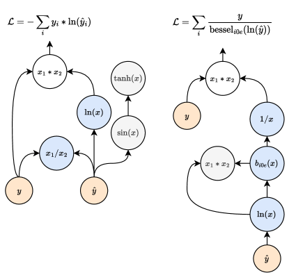
Figure 1: (Left) Example of how cross-entropy can be encoded using the search space. (Right) The exact encoding of the inverse bessel logarithm function in the search space. The root node is in white, while the active nodes are in blue, inactive nodes are in grey, and the final loss equation is given above the root node.

Algorithm 1 Regularized Evolution

1:  $population$ = RandomInitialization()

2:  $validationAcc$ = TrainModel($population$)

3:  repeat

4:     $winner$ = Tournament($population$, $validationAcc$)

5:     $child$ = Mutation($winner$)

6:     $valAcc$ = TrainModel($child$)

7:     $population$ = ReplaceOldest($population$, $child$)

8:     $validationAcc$ = Update($validationAcc$, $valAcc$)

9:  until Time Expired

3 Methodology

3.1 Image Augmentation Correlation

Because training each candidate loss function on a full scale model is extremely computationally expensive, surrogate functions can be used as proxies. It is typical to use smaller models, smaller datasets, and shortened training schedules when constructed surrogate functions (Zoph et al., 2018; Bingham et al., 2020; Bingham & Miikkulainen, 2022). Morgan & Hougen (2024) revealed the disparity of correlation between loss functions trained on smaller models and those trained on full scale models. Now, we investigate this observation further by taking a look at image augmentation techniques.

In order to assess how well loss functions transferred across image augmentation techniques, we constructed five different image augmentations. The first, referred to as base, served as the simplest form of image augmentation. In this augmentation, the images were zero-padded before a random crop equal to the training image size was obtained. The resulting image was then randomly horizontally flipped. The rest of the four image augmentations were built using base as the foundation. The second, referred to as cutout, applied the cutout operation, with a fixed patch size, to the image. The third, referred to as mixup, applied the mixup operation by creating artificial images through random linear combinations of images and their labels. The fourth, referred to as RandAug, applied the random augmentation strategy to randomly augment the images from a list of possible augmentations. Lastly, the fifth, referred to as all, combined all previous augmentations together in order to maximize regularization. Figure 2 shows an example of each augmentation on an image from the Oxford-Flowers dataset. As one can see, base only slightly alters the image, while all completely distorts it. Despite the massive distortion of the all augmentation, our results reveal that the all augmentation technique consistently outperforms the other four.

Figure 2: First Image: original untampered image. Second: base augmentation. Third: cutout augmentation. Fourth: mixup augmentation. Fifth: RandAug augmentation. Sixth: all augmentation

As with other neural component search methodologies, all searching experiments were performed on the CIFAR-10 dataset. For encouraging generalization, 5,000 of the 50,000 training images were set aside as validation. The validation accuracy is reported in all preliminary results. Using the search space, 1,000 random loss functions were generated and evaluated on the CIFAR-10 dataset. We did not have the computational resources to evaluate all loss functions on a state-of-the-art large-scale model; however, this does not mean we used a small model either. We chose to use a custom ResNet9v2 containing 6.5 million parameters as it was quick to train, while being relatively large (millions of parameters). The model was trained with the Adam optimizer (Kingma & Ba, 2014), batch size of 128, and one cycle cosine decay learning rate schedule (Smith, 2018) that warmed up the learning rate from zero to 0.001 after 1,000 steps, before being decayed back down to zero. The model was trained for 40 epochs, 500 steps per epoch, totalling to 20,000 steps.

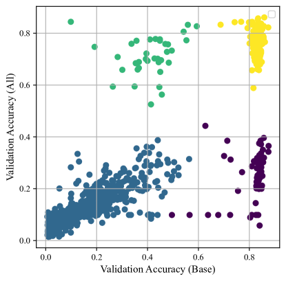
Figure 3: Validation accuracies for base and all techniques for the 1,000 randomly generated loss functions.

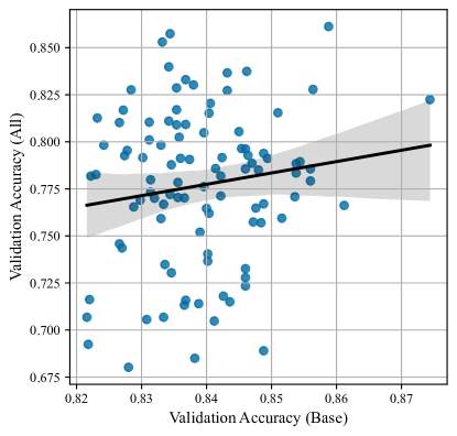
Figure 4: Validation accuracies for base and all techniques for the intersection of the best loss functions.

Figure 3 shows the scatter-plot of the validation accuracies for all 1,000 loss functions evaluated on base and all image augmentations. As one can see, there appear to be four clusters of loss functions after running agglomerative clustering with average linkage (colors denote different clusters). The first contain losses that do not perform well on either base ($<0.60$) nor all ($<0.50$). The second contain losses that perform well on base ($>0.80$) but not all ($<0.50$). The third contain losses that perform decently well on all ($>0.60$) but not well on base ($<0.60$). The last contain losses that perform well on base ($>0.75$) and decently well on all ($>0.60$). Because we care about preserving the rank in-between loss functions on different image augmentation techniques, we rely upon Kendall’s Tau rank correlation (Kendall, 1938). The top half of Table 3 gives the Tau rank correlation between all image augmentation techniques across all 1,000 randomly generated loss functions. As one can see, the rank correlations do not appear to poor, with the majority above $0.70$, signifying moderate to good rank preservation. However, Figure 3 shows that the majority of loss functions generated are degenerate, meaning the loss functions perform poorly on base ($<0.80$), all ($<0.60$), or both. During evolution, these loss functions would get filtered out due to the early stopping mechanism of the surrogate function. When the intersection of best 50 loss functions from base and all are joined together, the rank disparity becomes much more clearer. Figure 4 zooms in on the intersection of the best 50 loss functions from base and all. As one can see, the correlation seems almost uniform. The bottom half of Table 3 gives the Tau rank correlation between all image augmentation techniques across the intersection of the best 50 loss functions of each respective pair. These rank correlations are much lower, with all but one plummeting below $0.50$, indicating weak to moderate preservation of rank. Most noticeably, the rank correlations of base between all other image augmentation techniques, except RandAug, are extremely poor ($<0.10$). This disparity reveals that training loss functions with extremely little to no image augmentation (base) have no guarantee to transfer well to other forms of image augmentation, even when using the same model, dataset, and training strategy. Perhaps these results could explain the observation first noted by (Morgan & Hougen, 2024), where their smaller models ($<0.3$M parameters), trained without any image augmentation, transferred poorly to EfficientNetV2Small, trained with RandAug. Although, we cannot know this for certain without testing the effects of transferring loss functions across model size, this observation is important for all future NLFS endeavours, as it signifies that training loss functions with very little image augmentation may be predisposing them to lack the ability of effectively transferring to other augmentation techniques.

Table 3: Kendall Tau’s rank correlation between the five different image augmentation techniques for 1000 randomly generated loss functions evaluated on a ResNet9 (6.5M parameters). Top half of the table is the rank correlation for all 1000 loss functions. Bottom half is the rank correlation for best 50.

All Losses	Cutout	Mixup	RandAug	All
Base	0.773	0.711	0.743	0.711
Cutout	-	0.704	0.743	0.699
Mixup		-	0.692	0.736
RandAug			-	0.677
Best 50 Losses
Base	0.079	0.056	0.212	0.042
Cutout	-	0.309	0.590	0.357
Mixup		-	0.442	0.462
RandAug			-	0.482

3.2 Evolutionary Runs

From the results discussed in Section 3.1, we decided to capitalize on the disparity of rank correlation between image augmentation techniques by performing regularized evolution on each of the five proposed augmentation techniques in the hopes of finding image augmentation specific loss functions. Five evolutionary runs were performed, one for each technique. We used the same setup for our evolution as described by Morgan & Hougen (2024). The best 100 loss functions from the initial 1,000 randomly generated loss functions formed the first generation for each respective technique. With a tournament size of 20, the genetic algorithm was allowed to run for 2,000 iterations.

3.3 Elimination Protocol

In order to properly evaluate the final loss functions, we chose to compare the final functions on WideResNet-28-10 (36M parameters), a large scale state-of-the-art model. To ensure transferability across model sizes, we used a similar loss function elimination protocol to Morgan & Hougen (2024). The best 100 loss functions discovered over the entire evolutionary search for each run were retrained on the same surrogate function as before, except the training session was extended to 192 epochs instead of 40, totalling to 96,000 steps. The best 24 from that were taken and trained on WideResNet-28-10 for each respective technique. The best 12 from that were taken and trained again. The best 6, compared by averaging their two previous runs on WideResNet, from that were taken and trained again. Finally, the best three, compared by averaging their previous three runs on WideResNet, were chosen and presented. When training on WideResNet-28-10, the SGD optimizer was used, along with Nesterov’s momentum of 0.9, and a one cycle cosine decay learning rate schedule that warmed up the learning rate from zero to 0.1 after 1,000 steps, before being decayed back down to zero. The model was trained for 300 epochs, 391 steps per epoch, totalling to 117,300 steps.

4 Results

4.1 Final Losses

During our elimination protocol, the best 24 loss functions from the 100 trained on ResNet9v2 for 96,000 steps were trained on WideResNet for 117,300 steps. Using their final best validation accuracies for both models, we were able to construct the rank correlation to assess how well the loss functions would transfer to a larger model. Our results for base, cutout, mixup, RandAug, and all were 0.243, 0.034, 0.112, 0.307, and 0.100. As one can see, these are extremely poor, which confirms the original findings by Morgan & Hougen (2024) of poor correlation between smaller models and large CNNs. Despite this lack of correlation, the majority of our final found loss functions still performed well compared to CE.

The final three loss functions for each augmentation technique, base ($B0,B1,B2$), cutout ($C0,C1,C2$), mixup ($M0,M1,M2$), RandAug ($R0,R1,R2$), and all ($A0,A1,A2$), are shown in Table 4. From the table, a few observations can be made. First, all base, cutout, and RandAug functions used the expression $\hat{y}/(y+\epsilon)$. Second, all three of the all functions were of the form $f(\log(\hat{y}))*y$, where it was either $\log(x)$ or $\ln(x)$, and $f(x)$ was dependent upon the function. Lastly, many of the loss functions, across all five of the techniques, used some form of the bessel function. The binary phenotypes (when $y=1$) of the normalized loss values for a hand selected number of the final loss functions, based upon the results in Section 4.2, can be seen in Figure 5. As one can see, many of the final loss functions differ in their phenotype compared to CE, either in terms of learning a shifted global minimum or a much steeper or less steep slope.

Table 4: The final discovered loss functions.

Name	Loss Equation
B0	$-\frac{1}{n}\sum_{i}\sigma(\text{softplus}(\hat{y}_{i}/(y_{i}+\epsilon)))$
B1	$-\frac{1}{n}\sum_{i}\frac{d}{dx}\sigma(\text{bessel\_i0e}(\hat{y}_{i}/(y_{i}+\epsilon)))$
B2	$-\frac{1}{n}\sum_{i}\text{bessel\_i1e}(\text{erf}(\hat{y}_{i}/(y_{i}+\epsilon))$
C0	$-\frac{1}{n}\sum_{i}\ln(\arctan(\hat{y}_{i}/(y_{i}+\epsilon)))$
C1	$-\frac{1}{n}\sum_{i}\ln(\text{softplus}(\hat{y}_{i}/(y_{i}+\epsilon))$
C2	$-\frac{1}{n}\sum_{i}\sigma(\log(\hat{y}_{i}/(y_{i}+\epsilon)))$
M0	$-\frac{1}{n}\sum_{i}\text{bessel\_i1}(\arctan(\log(\hat{y}_{i})))*y_{i}$
M1	$\frac{1}{n}\sum_{i}\ln(1+\exp(\hat{y}_{i}-y_{i}))$
M2	$\frac{1}{n}\sum_{i}\text{arcsinh}(\text{bessel\_i0}(y_{i}-\hat{y}_{i}))$
R0	$\frac{1}{n}\sum_{i}\frac{d}{dx}\tanh(\text{bessel\_i0e}(\hat{y}_{i}/y_{i}+\epsilon))+\text{bessel\_i0e}(\hat{y}_{i}/y_{i})$
R1	$\frac{1}{n}\sum_{i}\log(\hat{y}_{i}/y_{i}+\epsilon)/\sqrt{1+(\log(\hat{y}_{i}/y_{i}+\epsilon)+y_{i})^{2}}$
R2	$\frac{1}{n}\sum_{i}|\log(\hat{y}_{i}/y_{i}+\epsilon)|^{|\text{bessel\_i0}(y_{i})|}$
A0	$-\frac{1}{n}\sum_{i}\ln(\frac{d}{dx}\text{softsign}(\log(\hat{y}_{i})))*y_{i}$
A1	$-\frac{1}{n}\sum_{i}\ln(\text{bessel\_i0e}(\log(\hat{y}_{i}))*y_{i}$
A2	$\frac{1}{n}\sum_{i}y_{i}/(\text{bessel\_i0e}(\ln(\hat{y}_{i}+\epsilon)))$
CE	$-\frac{1}{n}\sum_{i}y_{i}\ln\Bigl{(}|\hat{y}_{i}|+\epsilon\Bigr{)}$

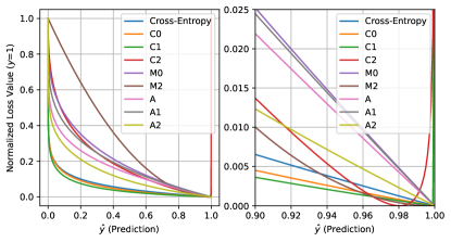
Figure 5: Binary phenotype of the final best loss functions against cross-entropy for normalized loss values.

4.2 Evaluation

To assess the quality of the final loss functions, all were trained on WideResNet-28-10 using the training strategy discussed in Section 3.3 on the CIFAR-10 and CIFAR-100 datasets. The results for the CIFAR datasets can be seen in Table 5. For comparison, cross-entropy (CE), both with and without label smoothing (CE_0.10, $\alpha=0.10$) were trained. From the table, a few observations arise. First, for CIFAR-10, not all loss functions evolved for each specific image augmentation technique outperformed CE for that technique. For example, all of the final RandAug loss functions performed poorly compared to CE on RandAug. On the contrary, some loss functions performed well on techniques that they were not evolved upon. For example, functions from the all group achieved Top 1 on base and mixup. Second, when transferring to CIFAR-100, all of the final functions for base and RandAug, and $M1$, collapse, performing extremely poorly. This observation reinforces the idea that loss functions evolved on a particular dataset, model, and training strategy may not perform well in other environments. Third, only twice did CE or CE_0.10 achieve Top 1 across all augmentation techniques on CIFAR-10 and CIFAR-100, indicating great success for the final loss functions.

To further assess the performance of the final loss functions on different datasets and architectures, the best overall performing functions from CIFAR-10 and CIFAR-100 were selected be fine-tuned on CARS-196 using EfficientNetV2Small and their official ImageNet2012 (Deng et al., 2009) published weights. The best overall functions were chosen to be all cutout and all functions, and $M0$ and $M2$. When fine-tuning on EfficientNetV2Small, the SGD optimizer was used, along with Nesterov’s momentum of 0.9, batch size of 64, and a one cycle cosine decay learning rate schedule that warmed up the learning rate from zero to 0.1 after 1,000 steps, before being decayed back down to zero. The models were trained for 20 epochs, 500 steps per epoch, totalling to 10,000 steps. The results are shown in Table 6. Once again, a few loss functions struggle to generalize, $C0$, $C2$, and $M2$. However, the $A2$ loss function performs relatively well compared to other discovered loss functions across all techniques. In fact, even combining $A2$ with a label smoothing value of $\alpha=0.10$, $A2_{0.10}$, achieves Top 1 for all techniques on CARS-196. The generalization power of $A2$ was further explored by being fine-tuned on Oxford-Flowers-102 and Caltech-101, as shown in Table 6. For these other two datasets, the best loss flipped between $A2_{0.10}$ and CE_0.10.

Table 5: Results for all final loss functions evaluated on the CIFAR datasets using each of the five selected image augmentation techniques. The mean and standard deviation of the test accuracy across 5 independent runs are reported. Red indicates Top 1 performance, while bold indicates Top 5 performance.

Loss	Base	Cutout	Mixup	RandAug	All
CIFAR-10
CE	94.116$\pm$0.238	95.400$\pm$0.107	96.616$\pm$0.600	95.012$\pm$0.261	96.258$\pm$0.227
CE0.10	94.080$\pm$0.245	95.326$\pm$0.240	96.598$\pm$0.576	94.864$\pm$0.199	96.368$\pm$0.244
b0	94.018$\pm$0.371	95.222$\pm$0.106	94.396$\pm$0.358	94.510$\pm$0.153	91.040$\pm$0.182
b1	94.272$\pm$0.175	95.324$\pm$0.066	95.212$\pm$0.397	94.628$\pm$0.226	92.400$\pm$0.110
b2	94.392$\pm$0.226	95.544$\pm$0.090	95.552$\pm$0.531	94.902$\pm$0.116	93.954$\pm$0.138
c0	94.446$\pm$0.202	95.600$\pm$0.154	95.934$\pm$0.441	95.022$\pm$0.169	95.076$\pm$0.148
c1	94.238$\pm$0.344	95.496$\pm$0.048	95.936$\pm$0.634	95.090$\pm$0.276	95.012$\pm$0.174
c2	94.454$\pm$0.212	95.710$\pm$0.141	95.030$\pm$0.482	95.164$\pm$0.143	93.284$\pm$0.181
m0	94.432$\pm$0.286	95.482$\pm$0.188	96.174$\pm$0.358	94.740$\pm$0.240	96.044$\pm$0.125
m1	94.446$\pm$0.141	95.528$\pm$0.097	96.162$\pm$0.435	95.092$\pm$0.202	95.268$\pm$0.080
m2	94.364$\pm$0.322	95.510$\pm$0.065	96.644$\pm$0.447	95.068$\pm$0.233	95.448$\pm$0.072
r0	94.250$\pm$0.267	95.434$\pm$0.165	93.136$\pm$0.404	94.660$\pm$0.227	89.364$\pm$0.253
r1	94.106$\pm$0.222	95.514$\pm$0.125	95.546$\pm$0.572	94.876$\pm$0.210	94.204$\pm$0.046
r2	93.704$\pm$0.344	95.172$\pm$0.184	95.486$\pm$0.468	93.858$\pm$0.263	92.550$\pm$0.123
a0	94.258$\pm$0.140	95.488$\pm$0.147	96.654$\pm$0.507	94.758$\pm$0.270	96.152$\pm$0.287
a1	94.566$\pm$0.178	95.390$\pm$0.130	96.086$\pm$0.081	94.866$\pm$0.249	96.110$\pm$0.185
a2	94.304$\pm$0.231	95.374$\pm$0.149	96.246$\pm$0.440	95.142$\pm$0.224	96.076$\pm$0.239
a20.10	93.946$\pm$0.276	95.270$\pm$0.100	96.644$\pm$0.519	94.898$\pm$0.243	96.418$\pm$0.19
CIFAR-100
CE	75.678$\pm$0.452	77.540$\pm$0.472	80.054$\pm$1.734	77.354$\pm$0.448	81.166$\pm$1.203
CE0.10	75.916$\pm$0.391	76.692$\pm$0.703	80.488$\pm$1.644	76.522$\pm$0.871	80.748$\pm$1.666
b0	59.652$\pm$1.505	41.734$\pm$0.602	45.960$\pm$0.833	31.988$\pm$0.425	31.988$\pm$0.425
b1	21.852$\pm$0.893	20.504$\pm$1.966	31.602$\pm$1.071	11.940$\pm$1.665	16.392$\pm$0.448
b2	54.822$\pm$2.624	22.892$\pm$2.199	78.464$\pm$1.162	22.892$\pm$2.199	49.318$\pm$1.225
c0	74.494$\pm$1.012	76.098$\pm$0.632	79.658$\pm$2.038	75.654$\pm$0.661	79.412$\pm$0.640
c1	75.748$\pm$0.600	76.410$\pm$0.656	79.498$\pm$2.454	75.934$\pm$0.844	79.288$\pm$0.787
c2	76.694$\pm$0.419	78.866$\pm$0.544	78.914$\pm$2.127	76.926$\pm$0.614	72.340$\pm$0.545
m0	75.670$\pm$0.495	77.290$\pm$0.626	79.670$\pm$1.849	75.850$\pm$0.524	79.394$\pm$0.907
m1	62.826$\pm$0.822	55.574$\pm$0.565	49.208$\pm$0.984	40.786$\pm$0.653	28.504$\pm$0.712
m2	76.430$\pm$0.585	77.278$\pm$0.533	74.998$\pm$1.387	61.574$\pm$1.980	40.036$\pm$0.251
r0	31.658$\pm$0.676	26.438$\pm$0.455	25.345$\pm$0.881	15.038$\pm$0.706	10.280$\pm$0.451
r1	17.732$\pm$1.834	30.760$\pm$1.598	46.834$\pm$1.729	15.120$\pm$0.117	12.291$\pm$0.374
r2	73.854$\pm$0.666	60.856$\pm$0.859	51.300$\pm$1.668	25.148$\pm$2.357	15.964$\pm$0.383
a0	75.552$\pm$0.606	76.798$\pm$0.550	78.810$\pm$1.971	75.272$\pm$0.253	80.320$\pm$1.475
a1	75.278$\pm$0.589	76.630$\pm$0.727	78.394$\pm$1.946	76.652$\pm$0.228	81.058$\pm$0.814
a2	76.034$\pm$0.771	77.486$\pm$0.460	80.252$\pm$2.101	77.020$\pm$0.729	79.378$\pm$0.427
a20.10	75.714$\pm$0.609	76.954$\pm$0.482	79.114$\pm$1.853	76.516$\pm$0.688	81.728$\pm$0.809

Table 6: Results for all final loss functions evaluated when fine-tuning using each of the five selected image augmentation techniques. The mean and standard deviation of the test accuracy across 5 independent runs are reported. Red indicates Top 1 performance, while bold indicates Top 5 performance.

Loss	Base	Cutout	Mixup	RandAug	All
Cars-196
CE	88.740$\pm$0.195	89.506$\pm$0.124	88.390$\pm$0.189	91.914$\pm$0.077	91.747$\pm$0.076
CE0.10	89.628$\pm$0.140	89.643$\pm$0.084	88.700$\pm$0.101	91.909$\pm$0.110	91.765$\pm$0.159
c0	53.212$\pm$34.32	81.129$\pm$1.577	85.646$\pm$0.185	83.592$\pm$1.707	90.902$\pm$0.098
c1	89.026$\pm$0.893	89.583$\pm$0.112	85.654$\pm$0.368	90.593$\pm$2.959	90.969$\pm$0.203
c2	77.766$\pm$0.532	69.161$\pm$0.493	61.137$\pm$0.782	46.126$\pm$1.119	31.501$\pm$0.425
m0	84.932$\pm$0.245	88.394$\pm$0.150	88.394$\pm$0.150	90.728$\pm$0.213	90.899$\pm$0.085
m2	72.459$\pm$1.016	36.426$\pm$1.270	36.426$\pm$1.270	58.866$\pm$1.864	11.800$\pm$1.122
a0	86.758$\pm$0.214	88.638$\pm$0.186	88.638$\pm$0.186	91.063$\pm$0.152	91.466$\pm$0.123
a1	87.136$\pm$0.283	88.019$\pm$0.165	88.780$\pm$0.116	91.071$\pm$0.056	91.404$\pm$0.135
a2	88.820$\pm$0.190	89.255$\pm$0.196	88.720$\pm$0.157	91.899$\pm$0.077	91.775$\pm$0.108
a20.10	89.810$\pm$0.117	89.909$\pm$0.259	88.999$\pm$0.122	91.989$\pm$0.095	91.780$\pm$0.172
Oxford-Flowers-102
CE	89.403$\pm$0.338	89.985$\pm$0.477	87.985$\pm$0.426	93.283$\pm$0.205	92.181$\pm$0.171
CE0.10	92.613$\pm$0.110	93.710$\pm$0.415	89.816$\pm$0.422	94.786$\pm$0.156	92.753$\pm$0.211
A2	89.605$\pm$0.228	89.855$\pm$0.663	88.769$\pm$0.331	93.644$\pm$0.333	92.340$\pm$0.273
A20.10	91.778$\pm$0.293	92.961$\pm$0.483	89.631$\pm$0.270	94.819$\pm$0.167	93.020$\pm$0.276
Caltech-101
CE	90.621$\pm$0.629	91.318$\pm$0.411	90.053$\pm$0.203	90.595$\pm$0.308	91.085$\pm$0.137
CE0.10	93.261$\pm$0.241	92.932$\pm$0.451	90.756$\pm$0.076	91.437$\pm$0.235	91.381$\pm$0.158
A2	90.510$\pm$0.578	91.032$\pm$0.233	90.746$\pm$0.220	90.756$\pm$0.174	91.561$\pm$0.232
A20.10	93.041$\pm$0.234	92.794$\pm$0.397	90.986$\pm$0.394	91.252$\pm$0.276	91.423$\pm$0.319

4.3 Inverse Bessel Logarithm Loss

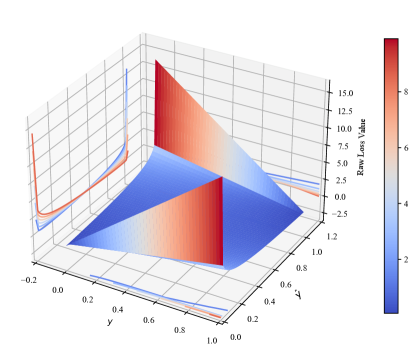
Figure 6: 3D plot of the raw phenotype of the cross-entropy loss.

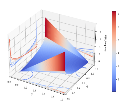
Figure 7: 3D plot of the raw phenotype of the $A2$ loss.

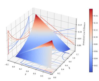
Figure 8: 3D plot of the difference in normalized loss values between $A2$ and cross-entropy ($A2-CE$).

Due to the success of $A2$ in terms of generalization across the CIFAR and fine-tuning datasets, it was deemed as the final best loss function discovered in this work, which we called the inverse bessel logarithm loss, due to its equation phenotype. The binary phenotypes of loss functions limit how well the loss landscape can be investigated for multiple dimensions. In order to better assess the differences between CE and the inverse bessel logarithm, a three-dimensional plot can be constructed where the $x$-axis takes on $y$ values, the $y$-axis takes on $\hat{y}$ values, and the $z$-axis takes on the loss $\mathcal{L}(y,\hat{y})$. Figure 6 shows the non-normalized three-dimensional representation of CE, while Figure 7 shows the non-normalized three-dimensional representation of inverse bessel logarithm. Visually, one can see that inverse bessel logarithm has a slight upward curve when $\hat{y}\sim 0$ and $\hat{y}\sim 1$. To better see this difference, Figure 8 shows the normalized three-dimensional difference between inverse bessel logarithm and CE. It can be seen that the largest differences occur right before $y$ and $\hat{y}$ are the most different (when $\hat{y}\to 0$ and $y\to 1$, or $\hat{y}\to 1$ and $y\to 0$). When $\hat{y}\sim 0$ and $y\sim 1$, the differences are extremely small. However, when $\hat{y}$ is slightly increased to $0.02$, the difference reaches its max value of $0.188$. As a result, it can be stated that inverse bessel logarithm has larger normalized loss values than CE when the model is almost at its most incorrect state. This typically occurs only during the very early stages of training, when the model is at its most incorrect state. Perhaps these larger normalized loss values allow the model to expedite maneuvering to a better loss landscape early on during training, as larger loss values directly increase the learning rate.

5 Conclusion

In this work, we further explored the results of recent work in NLFS that revealed a disparity of rank correlation of loss functions between smaller surrogate functions and large scale models with regularization. Specifically, we revealed another disparity that exists, the lack of rank correlation of loss functions between different image augmentation techniques. We showed that the best performing loss functions, from a set of randomly generated loss functions, across five different image augmentation techniques showed extremely poor rank correlation. We capitalized on this disparity by evolving loss functions on each respective augmentation technique in the hopes to find augmentation specific losses. In the end, we found a set of loss functions that outperformed cross-entropy across all image augmentation techniques, except one, on the CIFAR datasets. In addition, we found one loss function in particular ($A2$), which we call the inverse bessel logarithm, that performed extremely well when fine-tuning on three large scale image resolution datasets. Our code can be found here: https://github.com/OUStudent/EvolvingLossFunctionsImageAugmentation.

Appendix A Binary and Three Dimensional Phenotypes

In this appendix, the binary and three-dimensional phenotypes of the discovered loss functions will be covered.

A.1 Base Losses

The normalized and raw binary phenotypes of the final base losses are shown in Figure 9. The non-normalized three-dimensional representations for $B0$, $B1$, and $B2$ are shown in Figures 10, 11, and 12. As one can see, the base functions are extremely different from CE. Specifically, their slope values are much less steeper than CE. Their three-dimensional representations look like saddles. Perhaps these saddle representations pose problems at higher dimensions, more than one class, as all base functions collapse when transferring to CIFAR-100.

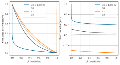
Figure 9: Binary Phenotype of the final Base losses against cross-entropy for both normalized and raw loss values.

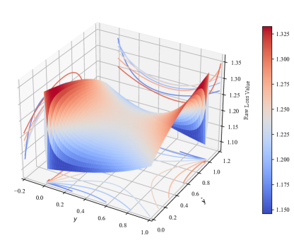
Figure 10: 3D plot of the raw phenotype of the $B0$ loss.

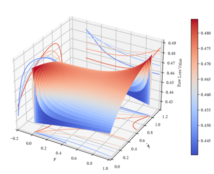
Figure 11: 3D plot of the raw phenotype of the $B1$ loss.

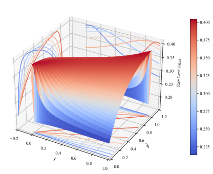
Figure 12: 3D plot of the raw phenotype of the $B2$ loss.

A.2 Cutout Losses

The normalized and raw binary phenotypes of the final cutout losses are shown in Figure 13. The non-normalized three-dimensional representations for $C0$, $C1$, and $C2$ are shown in Figures 14, 15, and 16. As one can see from the binary phenotypes, the final cutout functions learn a little hook around $\hat{y}\sim 1$, a small label smoothing value. Unlike the base losses, the cutout losses are not so similar in their three-dimensional representations, despite having similar binary phenotypes. For example, $C0$ and $C1$ are similar, but are very different from $C2$.

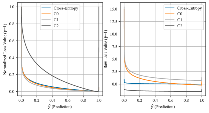
Figure 13: Binary Phenotype of the final Cutout losses against cross-entropy for both normalized and raw loss values.

Figure 14: 3D plot of the raw phenotype of the $C0$ loss.

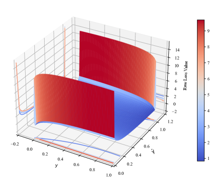
Figure 15: 3D plot of the raw phenotype of the $C1$ loss.

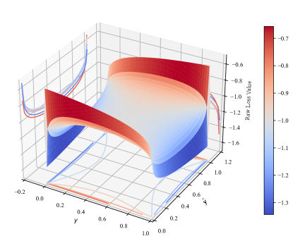
Figure 16: 3D plot of the raw phenotype of the $C2$ loss.

A.3 Mixup Losses

The normalized and raw binary phenotypes of the final mixup losses are shown in Figure 17. The non-normalized three-dimensional representations for $M0$, $M1$, and $M2$ are shown in Figures 18, 19, and 20. As one can see from the binary phenotypes, the final mixup loss functions learn less steeper slopes than CE. In addition, $M2$ and $M1$ appear to have the same normalized values, indicating that they have the exact same shape, but different scaling. From the three-dimensional representations, $M0$ is different from $M1$ and $M2$, better resembling CE, except with more exaggerated curves when $y$ and $\hat{y}$ are most different, resembling $A2$.

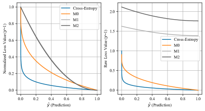
Figure 17: Binary Phenotype of the final Mixup losses against cross-entropy for both normalized and raw loss values.

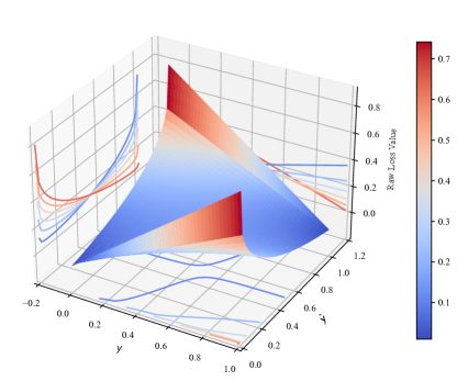
Figure 18: 3D plot of the raw phenotype of the $M0$ loss.

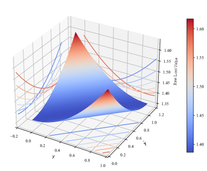
Figure 19: 3D plot of the raw phenotype of the $M1$ loss.

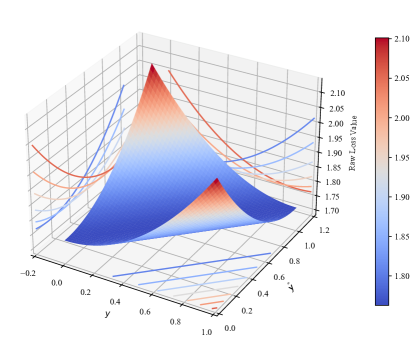
Figure 20: 3D plot of the raw phenotype of the $M2$ loss.

A.4 RandAug Losses

The normalized and raw binary phenotypes of the final mixup losses are shown in Figure 21. The non-normalized three-dimensional representations for $R0$, $R1$, and $R2$ are shown in Figures 22, 23, and 24. As one can see from the binary phenotypes, the final RandAug functions host a variety of differences within themselves. Mainly, $R0$ is the only loss function discovered where its maximum loss value does not occur when $\hat{y}=0$ for $y=1$, but actually when $\hat{y}=1$. Meaning, $R0$ gives the greatest penalty to when the model’s output directly matches the target. It seems that this level of regularization is too much for deep learning models as $R0$ performs extremely poorly on CIFAR-100.

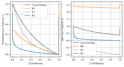
Figure 21: Binary Phenotype of the final RandAug losses against cross-entropy for both normalized and raw loss values.

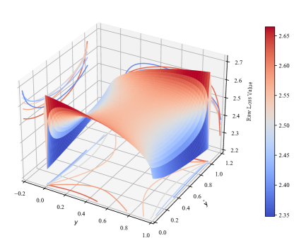
Figure 22: 3D plot of the raw phenotype of the $R0$ loss.

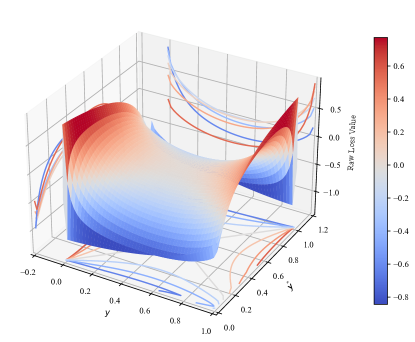
Figure 23: 3D plot of the raw phenotype of the $R1$ loss.

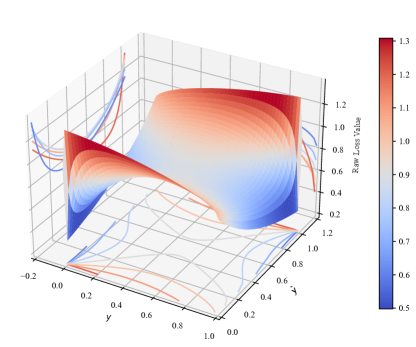
Figure 24: 3D plot of the raw phenotype of the $R2$ loss.

A.5 All Losses

The normalized and raw binary phenotypes of the final mixup losses are shown in Figure 25. The non-normalized three-dimensional representations for $A0$, $A1$, and $A2$ are shown in Figures 26 and 27. As one can see from the binary and three-dimensional phenotypes, the three final all functions are extremely similar in shape. The main difference is $A2$ has larger raw loss values. Empirically, these results seem to support the larger raw loss values as $A2$ consistently outperformed both $A0$ and $A1$.

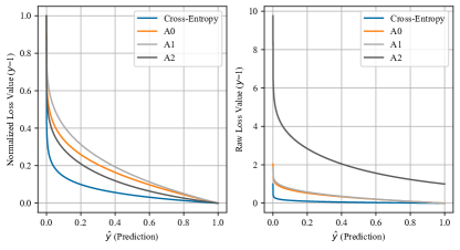
Figure 25: Binary Phenotype of the final All losses against cross-entropy for both normalized and raw loss values.

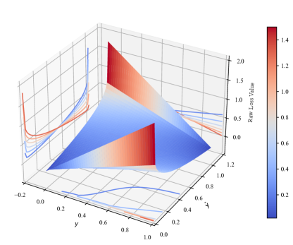
Figure 26: 3D plot of the raw phenotype of the $A0$ loss.

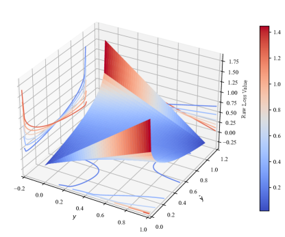
Figure 27: 3D plot of the raw phenotype of the $A1$ loss.

References

- Bingham & Miikkulainen (2022) Garrett Bingham and Risto Miikkulainen. Discovering parametric activation functions. Neural Networks, 148:48–65, 2022.
- Bingham et al. (2020) Garrett Bingham, William Macke, and Risto Miikkulainen. Evolutionary optimization of deep learning activation functions. In Proceedings of the 2020 Genetic and Evolutionary Computation Conference, GECCO ’20, pp. 289–296, New York, NY, USA, 2020. Association for Computing Machinery. ISBN 9781450371285. doi: 10.1145/3377930.3389841. URL https://doi.org/10.1145/3377930.3389841.
- Chebotar et al. (2019) Yevgen Chebotar, Artem Molchanov, Sarah Bechtle, Ludovic Righetti, Franziska Meier, and Gaurav S. Sukhatme. Meta learning via learned loss. In International Conference on Pattern Recognition (ICPR), pp. 4161–4168, 2019.
- Cubuk et al. (2018) Ekin D Cubuk, Barret Zoph, Dandelion Mane, Vijay Vasudevan, and Quoc V Le. Autoaugment: Learning augmentation policies from data. arXiv preprint arXiv:1805.09501, 2018.
- Cubuk et al. (2020) Ekin D Cubuk, Barret Zoph, Jonathon Shlens, and Quoc V Le. Randaugment: Practical automated data augmentation with a reduced search space. In Proceedings of the IEEE/CVF Conference on Computer Vision and Pattern Recognition Workshops, pp. 702–703, 2020.
- Deng et al. (2009) Jia Deng, Wei Dong, Richard Socher, Li-Jia Li, Kai Li, and Li Fei-Fei. Imagenet: A large-scale hierarchical image database. In 2009 IEEE Conference on Computer Vision and Pattern Recognition, pp. 248–255, 2009. doi: 10.1109/CVPR.2009.5206848.
- Fei-Fei et al. (2004) Li Fei-Fei, Rob Fergus, and Pietro Perona. Learning generative visual models from few training examples: An incremental Bayesian approach tested on 101 object categories. Computer Vision and Pattern Recognition Workshop, 2004.
- Gao et al. (2021) Boyan Gao, Henry Gouk, and Timothy M. Hospedales. Searching for robustness: Loss learning for noisy classification tasks. In Proceedings of the IEEE/CVF International Conference on Computer Vision (ICCV), pp. 6670–6679, October 2021.
- Gao et al. (2022) Boyan Gao, Henry Gouk, Yongxin Yang, and Timothy Hospedales. Loss function learning for domain generalization by implicit gradient. In Kamalika Chaudhuri, Stefanie Jegelka, Le Song, Csaba Szepesvari, Gang Niu, and Sivan Sabato (eds.), Proceedings of the 39th International Conference on Machine Learning, volume 162 of Proceedings of Machine Learning Research, pp. 7002–7016. PMLR, 17–23 Jul 2022. URL https://proceedings.mlr.press/v162/gao22b.html.
- Gonzalez & Miikkulainen (2020) Santiago Gonzalez and Risto Miikkulainen. Improved training speed, accuracy, and data utilization through loss function optimization. In 2020 IEEE Congress on Evolutionary Computation (CEC), pp. 1–8, 2020. doi: 10.1109/CEC48606.2020.9185777.
- Gonzalez & Miikkulainen (2021) Santiago Gonzalez and Risto Miikkulainen. Optimizing loss functions through multi-variate Taylor polynomial parameterization. In Proceedings of the Genetic and Evolutionary Computation Conference, GECCO ’21, pp. 305–313, New York, NY, USA, 2021. Association for Computing Machinery. ISBN 9781450383509. doi: 10.1145/3449639.3459277. URL https://doi.org/10.1145/3449639.3459277.
- Gu et al. (2022) Hongyang Gu, Jianmin Li, Guangyuan Fu, Chifong Wong, Xinghao Chen, and Jun Zhu. AutoLoss-GMS: Searching generalized margin-based softmax loss function for person re-identification. In Proceedings of the IEEE/CVF Conference on Computer Vision and Pattern Recognition (CVPR), pp. 4744–4753, June 2022.
- He et al. (2016) Kaiming He, Xiangyu Zhang, Shaoqing Ren, and Jian Sun. Identity mappings in deep residual networks. In European Conference on Computer Vision, pp. 630–645. Springer, 2016.
- Hinton et al. (2012a) Geoffrey E Hinton, Nitish Srivastava, Alex Krizhevsky, Ilya Sutskever, and Ruslan R Salakhutdinov. Improving neural networks by preventing co-adaptation of feature detectors. arXiv preprint arXiv:1207.0580, 2012a.
- Hinton et al. (2012b) Geoffrey E Hinton, Nitish Srivastava, Alex Krizhevsky, Ilya Sutskever, and Ruslan R Salakhutdinov. Improving neural networks by preventing co-adaptation of feature detectors. arXiv preprint arXiv:1207.0580, 2012b.
- Hinton et al. (2012c) Geoffrey E Hinton, Nitish Srivastava, Alex Krizhevsky, Ilya Sutskever, and Ruslan R Salakhutdinov. Improving neural networks by preventing co-adaptation of feature detectors. arXiv preprint arXiv:1207.0580, 2012c.
- Ho et al. (2019) Daniel Ho, Eric Liang, Xi Chen, Ion Stoica, and Pieter Abbeel. Population based augmentation: Efficient learning of augmentation policy schedules. In International conference on machine learning, pp. 2731–2741. PMLR, 2019.
- Kendall (1938) M. G. Kendall. A new measure of rank correlation. Biometrika, 30(1/2):81–93, 1938. ISSN 00063444. URL http://www.jstor.org/stable/2332226.
- Kingma & Ba (2014) Diederik P Kingma and Jimmy Ba. Adam: A method for stochastic optimization. arXiv preprint arXiv:1412.6980, 2014.
- Krause et al. (2013) Jonathan Krause, Michael Stark, Jia Deng, and Li Fei-Fei. 3d object representations for fine-grained categorization. In 4th International IEEE Workshop on 3D Representation and Recognition (3dRR-13), Sydney, Australia, 2013.
- Krizhevsky & Hinton (2009) Alex Krizhevsky and Geoffrey Hinton. Learning multiple layers of features from tiny images. Technical report, University of Toronto, Toronto, Ontario, 2009.
- Li et al. (2022) Hao Li, Tianwen Fu, Jifeng Dai, Hongsheng Li, Gao Huang, and Xizhou Zhu. Autoloss-zero: Searching loss functions from scratch for generic tasks. In 2022 IEEE/CVF Conference on Computer Vision and Pattern Recognition (CVPR), pp. 999–1008, 2022. doi: 10.1109/CVPR52688.2022.00108.
- Lin et al. (2017) Tsung-Yi Lin, Priya Goyal, Ross Girshick, Kaiming He, and Piotr Dollár. Focal loss for dense object detection. In Proceedings of the IEEE international conference on computer vision, pp. 2980–2988, 2017.
- Liu et al. (2021) Peidong Liu, Gengwei Zhang, Bochao Wang, Hang Xu, Xiaodan Liang, Yong Jiang, and Zhenguo Li. Loss function discovery for object detection via convergence-simulation driven search. arXiv preprint arXiv:2102.04700, 2021.
- Liu et al. (2022) Zhuang Liu, Hanzi Mao, Chao-Yuan Wu, Christoph Feichtenhofer, Trevor Darrell, and Saining Xie. A convnet for the 2020s. In Proceedings of the IEEE/CVF conference on computer vision and pattern recognition, pp. 11976–11986, 2022.
- Morgan & Hougen (2024) Brandon Morgan and Dean Hougen. Neural loss function evolution for large-scale image classifier convolutional neural networks. arXiv preprint arXiv, 2024.
- Müller et al. (2019) Rafael Müller, Simon Kornblith, and Geoffrey E Hinton. When does label smoothing help? Advances in neural information processing systems, 32, 2019.
- Nilsback & Zisserman (2008) M-E. Nilsback and A. Zisserman. Automated flower classification over a large number of classes. In Proceedings of the Indian Conference on Computer Vision, Graphics and Image Processing, Dec 2008.
- Raymond et al. (2022) Christian Raymond, Qi Chen, Bing Xue, and Mengjie Zhang. Learning symbolic model-agnostic loss functions via meta-learning. arXiv preprint arXiv:2209.08907, 2022.
- Real et al. (2019) Esteban Real, Alok Aggarwal, Yanping Huang, and Quoc V Le. Regularized evolution for image classifier architecture search. In Proceedings of the AAAI Conference on Artificial Intelligence, volume 33, pp. 4780–4789, 2019.
- Smith (2018) Leslie N Smith. A disciplined approach to neural network hyper-parameters: Part 1–learning rate, batch size, momentum, and weight decay. arXiv preprint arXiv:1803.09820, 2018.
- Tan & Le (2021) Mingxing Tan and Quoc Le. Efficientnetv2: Smaller models and faster training. In International Conference on Machine Learning, pp. 10096–10106. PMLR, 2021.
- Zagoruyko & Komodakis (2016) Sergey Zagoruyko and Nikos Komodakis. Wide residual networks. arXiv preprint arXiv:1605.07146, 2016.
- Zoph et al. (2018) Barret Zoph, Vijay Vasudevan, Jonathon Shlens, and Quoc V. Le. Learning transferable architectures for scalable image recognition. In Proceedings of the IEEE Conference on Computer Vision and Pattern Recognition (CVPR), June 2018.