Relative entropy bounds for sampling with and without replacement
Abstract
Sharp, nonasymptotic bounds are obtained for the relative entropy between the distributions of sampling with and without replacement from an urn with balls of colors. Our bounds are asymptotically tight in certain regimes and, unlike previous results, they depend on the number of balls of each colour in the urn. The connection of these results with finite de Finetti-style theorems is explored, and it is observed that a sampling bound due to Stam (1978) combined with the convexity of relative entropy yield a new finite de Finetti bound in relative entropy, which achieves the optimal asymptotic convergence rate.
1 Introduction
1.1 The problem
Consider an urn containing balls, each ball having one of different colours, and suppose we draw out of them. We will compare the difference in sampling with and without replacement. Write for the vector representing the number of balls of each colour in the urn, so that there are balls of colour , and . Write for the number of balls of each colour drawn out, so that .
When sampling without replacement, the probability that the colors of the balls drawn are given by is given by the multivariate hypergeometric probability mass function (p.m.f.),
| (1) |
for all with for all , and . In (1) and throughout, we write for the multinomial coefficient for any vector with .
Our goal is to compare with the corresponding p.m.f. of sampling with replacement, which is given by the multinomial distribution p.m.f.,
| (2) |
for all with and .
The study of the relationship between sampling with and without replacement has a long history and numerous applications in both statistics and probability; see, e.g., the classic review [22] or the text [24]. Beyond the elementary observation that and have the same mean, namely, that,
for each , it is well known that in certain limiting regimes the p.m.f.s themselves are close in a variety of senses. For example, Diaconis and Freedman [12, Theorem 4] show that and are close in the total variation distance :
| (3) |
In this paper we give bounds on the relative entropy (or Kullback-Leibler divergence) between and , which for brevity we denote as:
| (4) | |||||
[All logarithms are natural logarithms to base .] Clearly, if for some , then bounding becomes equivalent to the same problem with a smaller number of colours , so we may assume that each for simplicity.
Interest in controlling the relative entropy derives in part from the fact that it naturally arises in many core statistical problems, e.g., as the optimal hypothesis testing error exponent in Stein’s lemma; see, e.g., [9, Theorem 12.8.1]. Further, bounding the relative entropy also provides control of the distance between and in other senses. For example, Pinsker’s inequality, e.g. [26, Lemma 2.9.1], states that for any two p.m.f.s and ,
| (5) |
while the Bretagnolle-Huber bound [7, 8] gives:
Our results also follow along a long line of work that has been devoted to establishing probabilistic theorems in terms of relative entropy. Information-theoretic arguments often provide insights into the underlying reasons why the result at hand holds. Among many others, examples include the well-known work of Barron [4] on the information-theoretic central limit theorem; information-theoretic proofs of Poisson convergence and Poisson approximation [20]; compound Poisson approximation bounds [3]; convergence to Haar measure on compact groups [16]; connections with extreme value theory [18]; and the discrete central limit theorem [15]. We refer to [14] for a detailed review of this line of work.
The relative entropy in (4) has been studied before. Stam [23] established the following bound,
| (6) |
uniformly in , and also provided an asymptotically matching lower bound,
| (7) |
indicating that, in the regime and fixed , the relative entropy is of order .
More recently, related bounds were established by Harremoës and Matúš [17], who showed that (see [17, Theorem 4.5]),
| (8) |
and (see [17, Theorem 4.4]),
| (9) |
both results also holding uniformly in . Moreover, in the regime where and for all , they showed that the lower bound in (9) is asymptotically sharp and the upper bound in (8) is sharp to within a factor of 2 by proving that:
| (10) |
1.2 Main results
Despite the fact that (6) and (8) are both asymptotically optimal in the sense described above, it turns out it is possible to obtain more accurate upper bounds on if we allow them to depend on .111Indeed, as remarked by Harremoës and Matúš [17], “a good upper bound should depend on ” (in our notation). In this vein, our main result is the following; it is proved in Section 2.
Theorem 1.1.
For any , , and with and for each , the relative entropy between and satisfies:
| (11) | |||||
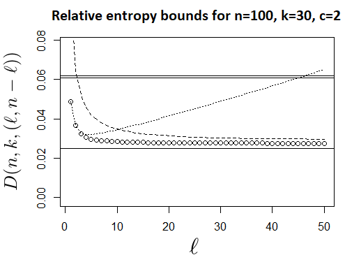
While the bound of Theorem 1.1 is simple, straightforward, and works well for the balanced cases described below, it is least accurate in the case of small ; see Figure 1. We therefore also provide an alternative expression in Proposition 1.2. For simplicity, we only give the result in the case , though similar arguments will work in general. It is proved in Appendix A.3.
Proposition 1.2.
Under the assumptions of Theorem 1.1, if and , we have:
Figure 1 shows a comparison of the earlier uniform bounds (6), (7) and (8), with the new bounds in Theorem 1.1 and Proposition 1.2, for the case , , and , for . It is seen that the combination of the two new upper bounds outperforms the earlier ones in the entire range of values considered.
Remarks.
-
1.
The dependence of the bound (11) in Theorem 1.1 on is only via the quantities:
(12) For , in the ‘balanced’ case where each , we have , and using Jensen’s inequality it is easy to see that we always have . In fact, the Schur-Ostrowski criterion shows that (12) is Schur convex, and hence respects the majorization order, being largest in ‘unbalanced’ cases. For example, if and , then as . On the other hand, in the regime considered by Harremoës and Matúš [17] where all for some , we have , which is bounded in .
Similar comments apply to : It is bounded in balanced cases, including the scenario of Harremoës and Matúš [17], but can grow like in the very unbalanced case.
-
2.
The first term in the bound (11) of Theorem 1.1,
matches the asymptotic expression in (10), so Theorem 1.1 may be regarded as a nonasymptotic version version of (10). In particular, (10) is only valid in the asymptotic case where all , when, as discussed above, is bounded. Therefore, in this balanced case Theorem 1.1 recovers the asymptotic result of (10).
-
3.
Any bound that holds uniformly in must hold in particular for the binary case with . Then is Bernoulli with parameter and is binomial with parameters and , and direct calculation gives the exact expression:
Taking while for some fixed , in this unbalanced case where and , we obtain:
(13) Compared with the analogous limiting expression (10) in the balanced case where are both bounded below by , this suggests that the asymptotic behaviour of in the regime may vary by a factor of 2 over different values of .
- 4.
1.3 Finite de Finetti theorems
Diaconis [11] and Diaconis and Freedman [12] revealed an interesting and intimate connection between the problem of comparing sampling with and without replacement, and finite versions of de Finetti’s theorem. Recall that de Finetti’s theorem says that the distribution of a infinite collection of exchangeable random variables can be represented as a mixture over independent and identically distributed (i.i.d.) sequences; see, e.g., [19] for an elementary proof in the binary case. Although such a representation does not always exist for finite exchangeable sequences, approximate versions are possible: If are exchangeable, then the distribution of is close to a mixture of independent sequences as long as is relatively small compared to . Indeed, Diaconis and Freedman [12] proved such a finite de Finetti theorem using the sampling bound (3).
Let be an alphabet of size , and suppose that the random variables , with values , are exchangeable, that is, the distribution of is the same as that of for any permutation on . Given a sequence of length , its type [10] is the vector of its empirical frequencies: The th component of is:
The sequence induces a measure on p.m.f.s on , via:
| (14) |
This is the law of the empirical measure induced by on .
For each , let denote the joint p.m.f. of , and write,
| (15) |
for the mixture of the i.i.d. distributions with respect to the mixing measure . A key step in the connection between sampling bounds and finite de Finetti theorems is the simple observation that, given that its type , the exchangeable sequence is uniformly distributed on the set of sequences with type . In other words, for any ,
| (16) |
where . This elementary and rather obvious (by symmetry) observation already appears implicitly in the literature, e.g., in [11, 14].
An analogous representation can be easily seen to hold for . Since the probability of an i.i.d. sequence only depends on its type, for any we have, with :
| (17) |
The following simple proposition clarifies the connection between finite de Finetti theorems and sampling bounds. Its proof is a simple consequence of (16) combined with (17) and the log-sum inequality [9].
Proposition 1.3.
Proof.
Fix with . The log-sum inequality gives that for any of type :
Hence, summing over the vectors of type we obtain,
Finally, summing over yields,
and each of the relative entropy terms can be bounded by the maximum value. ∎
Corollary 1.4 (Sharp finite de Finetti).
Under the assumptions of Proposition 1.3, for :
| (18) |
Pinsker’s inequality (5) and (18) gives,
In the regime this is in fact optimal, in that it is of the same order as Diaconis and Freedman’s [12] bound,
| (19) |
which they show is of optimal order in and when .
For certain applications, for example to approximation schemes for minimization of specific polynomials [5], the dependence on the alphabet size is also of interest; see also [6] and the references therein. The lower bound (7) shows that the linear dependence on the alphabet size is optimal for the sampling problem, in the sense that any upper bound that holds for any , , and , must have at least linear dependence on . However, we do not know whether the linear dependence on the alphabet size is optimal for the de Finetti problem under optimal rates in .
Information-theoretic proofs of finite de Finetti theorems have been lately developed in [13, 14, 6]. In [13], the bound,
| (20) |
was obtained for binary sequences, and in [14], the weaker bound,
| (21) |
was established for finite-valued random variables. Finally the sharper bound,
| (22) |
was derived in [6], where random variables with values in abstract spaces were also considered. Although the derivations of (20)–(22) are interesting in that they employ purely information-theoretic ideas and techniques, the actual bounds are of strictly weaker rate than the sharp rate we obtained in Corollary 1.4 via sampling bounds.
A question on monotonicity. A significant development in the area of information-theoretic proofs of probabilistic limit theorems was in 2004, when it was shown [2] that the convergence in relative entropy established by Barron in 1986 [4] was in fact monotone. In the present setting we observe that, while the total variation bound (19) of Diaconis and Freedman [12] is nonincreasing in , we do not know whether the total variation distance is itself monotone.
Writing , where the vector is distributed according to , a direct application of the data processing inequality for the relative entropy [9] gives that, for any integer :
In other words, is nondecreasing in . Since the total variation is an -divergence and therefore satisfies the data processing inequality, the same argument shows that is also nondecreasing in . In view of the monotonicity in the information-theoretic central limit theorem and the convexity properties of the relative entropy it is tempting to conjecture that is also nonincreasing in . However, this relative entropy depends on through the choice of the mixing measure , which makes the problem significantly harder. We therefore ask:
Let be a finite exchangeable random sequence and let the mixing measures be the laws of the empirical measures induced by and , respectively. For a fixed , is ? Are there possibly different measures such that is vanishing for and nonincreasing in ?
2 Upper bounds on relative entropy
The proof of Theorem 1.1 in this section will be based on the decomposition of as a sum of expectations of terms involving the quantity introduced in Definition 2.2. We tightly approximate these terms within a small additive error (see Proposition 2.3), and control the expectations of the resulting terms using Lemmas 2.4 and 2.5.
2.1 Hypergeometric properties
We first briefly mention some standard properties of hypergeometric distributions that will help our analysis.
Notice that (1) and (2) are both invariant under permutation of colour labels. That is, and , whenever and for the same permutation . Hence from (4) is itself permutation invariant,
| (23) |
so we may assume, without loss of generality, that . Similarly, if we swap the roles of balls that are ‘drawn’ and ‘not drawn’, then direct calculation using the second representation in (1) shows that,
| (24) |
Let . Then each has a multinomial distribution with , with p.m.f. given by .
We use standard notation and write for the falling factorial, and note that on marginalizing we can apply a standard result:
Lemma 2.1.
For any and , the factorial moments of the hypergeometric satisfy:
Hence, as mentioned in the Introduction, the mean . In general, we write for the th centered moment of and note that, by expressing as a linear combination of factorial moments of , we obtain that,
| (25) | |||||
| (26) |
2.2 Proof of Theorem 1.1
A key role in the proof will be played by the analysis of the following quantity, defined in terms of the gamma function :
Definition 2.2.
For , define the function:
| (27) |
Using the standard fact that , when and are both integers we can write,
and note that for all . Using Stirling’s approximation for the factorials suggests that , but we can make this precise using results of Alzer [1], for example. Proposition 2.3 is proved in Appendix A.1.
Proposition 2.3.
Writing,
for any we have the bounds:
| (28) |
Proof of Theorem 1.1.
We can give an expression for the relative entropy by using the second form of (1) and the fact that , to obtain,
so that we can express,
| (29) |
where has a hypergeometric distribution.222Note that since, , in the case all of the values involved in this calculation are of the form or , so (29) is identically zero as we would expect – we only sample one item, so it does not matter whether that is with or without replacement. Now, we can approximate by , to rewrite:
| (30) |
We bound the two parts of (30) in Lemmas 2.4 and 2.5, respectively. The result follows on combining these two expressions, noting that the result also includes the negative term,
which may be ignored. ∎
Lemma 2.4.
The first term of (30), , is bounded above by:
Lemma 2.5.
The second term in (30) is bounded above as:
Appendix A Appendix: Proofs
A.1 Proof of Proposition 2.3
The key to the proof is to work with the logarithmic derivative of the gamma function , . For completeness, we state and prove the following standard bound on :
Lemma A.1.
For any :
Proof.
A.2 Proofs of Lemmas 2.4 and A.2
Proof of Lemma 2.4.
In order to prove Lemma 2.5 we first provide a Taylor series based approximation for the summands in (30):
Lemma A.2.
Each term in the second sum in (30) satisfies:
| (34) | |||||
Proof.
Proof of Lemma 2.5.
We will bound the two terms from Lemma A.2. Using [1, Theorem 9] we can deduce that, for any ,
Hence, recalling the value of from (25), we know that the first term of (34) contributes an upper bound of,
| (36) | |||||
| (37) | |||||
where we used the fact that .
Since by assumption, we know from (26) that has the same sign as . And since, as described in (23), we can assume that , we know that for all , and hence . This means that, since is increasing in , we can bound each so that:
| (38) |
Finally, writing , we have that is concave and minimized at and . Therefore, the sum is minimized overall when and , giving the value . This means that , so (38) is negative, and we can simply use (37) as an upper bound. ∎
A.3 Proofs for small
Recall the form of the Newton series expansion; see, for example [21, Eq. (8), p. 59]:
Lemma A.3.
Consider a function for some . Suppose that, for some positive integers , and , the st derivative of is negative for all . Then, for any integer satisfying , there exists some such that:
where as before represents the falling factorial and is the th compounded finite difference where, as usual .
Lemma A.4.
For we have the upper bound:
| (39) |
Proof.
We write , and use Lemma A.3 with for fixed .
Remark A.5.
Note that (39) remains valid for as well, as long as we interpret the two bracketed terms in the bound appropriately: For we assume that both brackets are zero, which is consistent with the fact that , so the expectation is zero. For , the first bracket equals and again we assume the second bracket is zero. This is consistent with the fact that and , coupled with the fact that
References
- [1] H. Alzer. On some inequalities for the gamma and psi functions. Math. Comput., 66(217):373–389, 1997.
- [2] S. Artstein, K. Ball, F. Barthe, and A. Naor. Solution of Shannon’s problem on the monotonicity of entropy. J. Amer. Math. Soc., 17(4):975–982, April 2004.
- [3] A.D. Barbour, O. Johnson, I. Kontoyiannis, and M. Madiman. Compound Poisson approximation via information functionals. Electron. J. Probab, 15:1344–1369, August 2010.
- [4] A.R. Barron. Entropy and the central limit theorem. Ann. Probab., 14(1):336–342, January 1986.
- [5] M. Berta, F. Borderi, O. Fawzi, and V.B. Scholz. Semidefinite programming hierarchies for constrained bilinear optimization. Math. Program., 194(1-2):781–829, July 2022.
- [6] M. Berta, L. Gavalakis, and I. Kontoyiannis. A third information-theoretic approach to finite de Finetti theorems. arXiv e-prints, 2304.05360 [cs.IT], April 2023.
- [7] J. Bretagnolle and C. Huber. Estimation des densités: Risque minimax. Séminaire de probabilités XII 1976/77, pages 342–363, 1978.
- [8] C.L. Canonne. A short note on an inequality between KL and TV. arXiv e-prints, 2202.07198 [math.PR], February 2022.
- [9] T.M. Cover and J.A. Thomas. Elements of information theory. John Wiley & Sons, New York, NY, second edition, 2012.
- [10] I. Csiszár. The method of types. IEEE Trans. Inform. Theory, 44(6):2505–2523, October 1998.
- [11] P. Diaconis. Finite forms of de Finetti’s theorem on exchangeability. Synthese, 36(2):271–281, 1977.
- [12] P. Diaconis and D.A. Freedman. Finite exchangeable sequences. Ann. Probab., 8(4):745–764, 1980.
- [13] L. Gavalakis and I. Kontoyiannis. An information-theoretic proof of a finite de Finetti theorem. Electron. Comm. Probab., 26:1–5, 2021.
- [14] L. Gavalakis and I. Kontoyiannis. Information in probability: Another information-theoretic proof of a finite de Finetti theorem. In J.-M. Morel and B. Teissier, editors, Mathematics Going Forward: Collected Mathematical Brushstrokes, volume LNM 2313 of Lecture Notes in Mathematics. Springer, May 2023.
- [15] L. Gavalakis and I. Kontoyiannis. Entropy and the discrete central limit theorem. Stoch. Proc. Appl., 170:104294, June 2024.
- [16] P. Harremoës. Maximum entropy on compact groups. Entropy, 11(2):222–237, 2009.
- [17] P. Harremoës and F. Matús̆. Bounds on the information divergence for hypergeometric distributions. Kybernetika, 56(6):1111–1132, 2020.
- [18] O. Johnson. Information-theoretic convergence of extreme values to the Gumbel distribution. J. Appl. Probab., 61(1):244–254, 2024.
- [19] W. Kirsch. An elementary proof of de Finetti’s theorem. Statist. Probab. Lett., 151:84–88, 2019.
- [20] I. Kontoyiannis, P. Harremoës, and O. Johnson. Entropy and the law of small numbers. IEEE Trans. Inform. Theory, 51(2):466–472, February 2005.
- [21] L.M. Milne-Thomson. The calculus of finite differences. American Mathematical Society, Providence, RI, 2000.
- [22] J.N.K. Rao. On the comparison of sampling with and without replacement. Review of the International Statistical Institute, 34(2):125–138, 1966.
- [23] A.J. Stam. Distance between sampling with and without replacement. Statistica Neerlandica, 32(2):81–91, June 1978.
- [24] S.K. Thompson. Sampling. John Wiley & Sons, Hoboken, NJ, 2012.
- [25] F. Topsøe. Some bounds for the logarithmic function. In Y.J. Cho, J.K. Kim, and S.S. Dragomir, editors, Inequality Theory and Applications, volume 4, pages 137–151. Nova Science Publishers, New York, NY, 2007.
- [26] A.B. Tsybakov. Introduction to nonparametric estimation. Springer, New York, NY, 2009. Revised and extended from the orignal 2004 French edition. Translated by V. Zaiats.