Adapted optimal transport between Gaussian processes in discrete time

Abstract.

We derive explicitly the adapted $2$-Wasserstein distance between non-degenerate Gaussian distributions on $\mathbb{R}^{N}$ and characterize the optimal bicausal coupling(s). This leads to an adapted version of the Bures-Wasserstein distance on the space of positive definite matrices.

1. Introduction

Adapted (by which we mean bicausal) optimal transport (AOT) has emerged to be a useful tool for quantifying distributional uncertainty and the sensitivity of stochastic optimization problems in contexts where the flow of information in time plays a crucial role. The key idea, which has several origins in different fields, is to impose a (bi)causal constraint on the feasible couplings. We recall the necessary concepts in Section 2 and refer the reader to [3, 5, 4, 6, 9, 14, 18, 24], and the references therein, for detailed expositions of the theory and the related literature.

Several AOT problems have been explicitly solved. For example, [6] provides a sufficient condition for the Knothe-Rosenblatt coupling (recalled in Section 3) to be optimal in discrete time. Also see [7, 12, 18, 25] for continuous time results concerning stochastic differential equations. The main purpose of this paper is to address the adapted $2$-Wasserstein transport between arbitrary non-degenerate Gaussian measures on $\mathbb{R}^{N}$ which are possibly non-Markovian. To the best of our knowledge, this basic case is still open despite the rapid growth of the subject in recent years. The closest papers we could find are [16], which studies a distributionally robust filtering problem with Gaussian noise, and [28], which solves a related OT problem between stationary Gaussian processes.

Theorem 1.1.

Let $\mu=\mathcal{N}(a,A)$ and $\nu=\mathcal{N}(b,B)$ be non-degenerate Gaussian distributions on $\mathbb{R}^{N}$. Let $A=LL^{\top}$ and $B=MM^{\top}$ be the Cholesky decompositions of $A$ and $B$ respectively. Then the adapted $2$-Wasserstein distance $\mathcal{AW}_{2}(\mu,\nu)$ is given by

(1.1) $$\mathcal{AW}_{2}^{2}(\mu,\nu)=\|a-b\|^{2}+d_{\mathrm{ABW}}^{2}(A,B),$$

where $d_{\mathrm{ABW}}$ is the adapted Bures-Wasserstein distance on the space $\mathscr{S}_{++}(N)$ of positive definite matrices defined by

(1.2) $$d_{\mathrm{ABW}}^{2}(A,B):=\operatorname{tr}(A)+\operatorname{tr}(B)-2\|\operatorname{diag}(L^{\top}M)\|_{1}.$$

Here $\operatorname{diag}(\cdot)$ gives the diagonal of a square matrix, $\|\cdot\|_{1}$ is the $\ell_{1}$-norm and $\|\cdot\|=\|\cdot\|_{2}$ is the Euclidean norm.

After reviewing the Knothe-Rosenblatt coupling in Section 3, we prove Theorem 1.1 in Section 4 using a dynamic programming principle from [6] and characterize the optimal bicausal couplings in Corollary 4.4. Since the Gaussian distribution is fundamental in various applications, our explicit solution may improve the understanding of the general theory and stimulate new applications of AOT. We also note that Knothe-Rosenblatt transport maps (also called monotone triangular transport maps) have found recent applications in statistics and machine learning [2, 8]. Some geometric properties of the adapted Bures-Wasserstein distance are discussed in Section 5. Section 6 provides illustrative examples. Finally, we discuss some future directions in Section 7.

2. Adapted optimal transport

We work with Borel probability measures on $\mathbb{R}^{N}$, $N\in\mathbb{N}$, regarded as laws of real-valued stochastic processes indexed by $t\in[N]:=\{1,\ldots,N\}$. We use $\mathcal{P}(E)$ to denote the collection of Borel probability measures on a space $E$. By a coupling of $(\mu,\nu)\in(\mathcal{P}(\mathbb{R}^{N}))^{2}$ we mean an element $\pi\in\mathcal{P}(\mathbb{R}^{N}\times\mathbb{R}^{N})$ whose first and second marginals are $\mu$ and $\nu$ respectively. The set of couplings of $(\mu,\nu)$ is denoted by $\Pi(\mu,\nu)$. By an abuse of terminology we also use the word coupling to mean a pair $(X=(X_{t})_{t=1}^{N},Y=(Y_{t})_{t=1}^{N})$ of real-valued processes, defined on some probability space, with joint law $\pi\in\Pi(\mu,\nu)$. We write $\mathbb{P}_{\pi}$ for a probability under which $(X,Y)\sim\pi$ (analogous for $\mathbb{E}_{\pi}$).

For integers $s\leq t$ we let $s:t=(s,s+1,\ldots,t)$. We also write $\mathbf{t}=1:t$ and $\mathbf{t}^{\prime}=(t+1):N$. For a quantity $Z$ indexed by time we use the shorthand $Z_{s:t}=(Z_{s},\ldots,Z_{t})$ (by convention $Z_{1:0}$ is empty). Suppose $\mu\in\mathcal{P}(\mathbb{R}^{N})$ and $X\sim\mu$. For $t\in[N]$ we let $\mu_{t}(\cdot)\in\mathcal{P}(\mathbb{R})$ be the marginal distribution of $X_{t}$. For $x_{1:t}\in\mathbb{R}^{t}$, we let $\mu_{t+1}(\cdot|x_{1:t})\in\mathcal{P}(\mathbb{R})$ be the conditional distribution of $X_{t+1}$ given $X_{1:t}=x_{1:t}$, and let $\mu_{\mathbf{t}^{\prime}}(\cdot|x_{\mathbf{t}})\in\mathcal{P}(\mathbb{R}^{N-t})$ be the conditional distribution of $X_{\mathbf{t}^{\prime}}$ given $X_{\mathbf{t}}=x_{\mathbf{t}}$. Analogously, we define $\nu_{t+1}(\cdot|y_{\mathbf{t}})$ and $\nu_{\mathbf{t}^{\prime}}(\cdot|y_{\mathbf{t}})$ for $Y$, as well as $\pi_{t+1}(\cdot|x_{\mathbf{t}},y_{\mathbf{t}})$ and $\pi_{{\bf t}^{\prime}}(\cdot|x_{\mathbf{t}},y_{\mathbf{t}})$ for $(X,Y)$. These (regular) conditional kernels are well-defined by the disintegration theorem and are a.s. unique with respect to suitable reference measures.

Let $\mathcal{P}_{2}(\mathbb{R}^{N})=\{\mu\in\mathcal{P}(\mathbb{R}^{N}):\int_{\mathbb{R}^{N}}\|x\|^{2}\mu(\mathrm{d}x)<\infty\}$ be the collection of probability measures on $\mathbb{R}^{N}$ with finite second moment. For $\mu,\nu\in\mathcal{P}_{2}(\mathbb{R}^{N})$, the usual $2$-Wasserstein distance $\mathcal{W}_{2}(\mu,\nu)$ is defined by

(2.1) $$\mathcal{W}_{2}^{2}(\mu,\nu)=\inf_{\pi\in\Pi(\mu,\nu)}\int_{\mathbb{R}^{N}\times\mathbb{R}^{N}}\|x-y\|^{2}\mathrm{d}\pi(x,y).$$

We simply call $\mathcal{W}_{2}$ the Wasserstein distance since $2$ is the only order considered in this paper (similar for other quantities such as the Knothe-Rosenblatt distance (3.2)). Let $\mathscr{S}_{++}(N)$ (resp. $\mathscr{S}_{+}(N)$) be the space of $N$-by-$N$ positive definite (resp. semipositive definite) matrices. When $\mu=\mathcal{N}(a,A)$ and $\nu=\mathcal{N}(b,B)$ are Gaussian distributions on $\mathbb{R}^{N}$, it is well known that

(2.2) $$\mathcal{W}_{2}^{2}(\mu,\nu)=\|a-b\|^{2}+d_{\mathrm{BW}}^{2}(A,B),$$

where $d_{\mathrm{BW}}$ is the Bures-Wasserstein distance on $\mathscr{S}_{+}(N)$ defined by

(2.3) $$d_{\mathrm{BW}}^{2}(A,B)=\operatorname{tr}(A)+\operatorname{tr}(B)-2\operatorname{tr}\big{(}A^{\frac{1}{2}}BA^{\frac{1}{2}}\big{)}^{\frac{1}{2}}.$$

Here $A^{\frac{1}{2}}\in\mathscr{S}_{+}(N)$ is the unique matrix square root of $A\in\mathscr{S}_{+}(N)$. See [11, 20, 27] for in-depth studies of $d_{\mathrm{BW}}$ from the viewpoints of matrix analysis and Riemannian geometry. When $A,B\in\mathscr{S}_{++}(N)$ the value $\mathcal{W}_{2}^{2}(\mu,\nu)$ is achieved uniquely by the deterministic coupling $Y=T_{\mathrm{W}}^{\mu,\nu}X$, where $X\sim\mu$ and

(2.4) $$T_{\mathrm{W}}^{\mu,\nu}x=b+A^{-\frac{1}{2}}\big{(}A^{\frac{1}{2}}BA^{\frac{1}{2}}\big{)}^{\frac{1}{2}}A^{-\frac{1}{2}}(x-a).$$

Here and below we use the column convention for $X$, $Y$, etc. When $N=1$ this reduces to the comonotonic coupling with transport map $T_{\mathrm{W}}^{\mu,\nu}=F_{\nu}^{-1}\circ F_{\mu}$, where $F$ denotes the distribution function. For later use we also recall the counter-monotonic coupling which has transport map $F_{\nu}^{-1}\circ R\circ F_{\mu}$, where $R(u)=1-u$. Note that the Jacobian matrix in (2.4) is an element of $\mathscr{S}_{++}(N)$ since $T_{\mathrm{W}}^{\mu,\nu}$ is a convex gradient. Unless it is diagonal, the transport map “looks into the future of $X$” since generally each $Y_{t}$ is a function of both $X_{\mathbf{t}}$ and $X_{\mathbf{t}^{\prime}}$. The causal condition excludes such couplings.

Definition 2.1 (Causal and bicausal couplings).

Let $\mu,\nu\in\mathcal{P}(\mathbb{R}^{N})$. A coupling $\pi\in\Pi(\mu,\nu)$ is said to be causal in the direction $\mu$ to $\nu$, if for all $t\in[N]$ and Borel $B\subset\mathbb{R}^{t}$ we have

$$\mathbb{P}_{\pi}(Y_{1:t}\in B|X_{1:N})=\mathbb{P}_{\pi}(Y_{1:t}\in B|X_{1:t}).$$

We say that $\pi$ is bicausal if it is causal in both directions, and let $\Pi_{bc}(\mu,\nu)$ be the collection of bicausal couplings of $(\mu,\nu)$.

We cite a useful equivalent condition, taken from [6, Proposition 5.1], for the bicausal property. Given $\pi\in\Pi(\mu,\nu)$, we decompose it as a product of regular conditional distributions (kernels):

(2.5) $$\begin{split}\pi(\mathrm{d}x_{1:N},\mathrm{d}y_{1:N})&=\pi_{1}(\mathrm{d}x_{1},\mathrm{d}y_{1})\pi_{2}(\mathrm{d}x_{2},\mathrm{d}y_{2}|x_{1},y_{1})\\ &\quad\quad\cdots\pi_{N}(\mathrm{d}x_{N},\mathrm{d}y_{N}|x_{1:(N-1)},y_{1:(N-1)}).\end{split}$$

Then $\pi\in\Pi_{bc}(\mu,\nu)$ if and only if $\pi_{1}\in\Pi(\mu_{1},\nu_{1})$ and, for all $2\leq t\leq N$ and ($\pi$-almost) all $x_{1:t},y_{1:t}\in\mathbb{R}^{t}$, we have

$$\pi_{t+1}(\cdot|x_{1:t},y_{1:t})\in\Pi(\mu_{t+1}(\cdot|x_{1:t}),\nu_{t+1}(\cdot|y_{1:t})).$$

In [26] this is called a Markov-construction. If in (2.1) we optimize over bicausal couplings we obtain the adapted Wasserstein distance.

Definition 2.2 (Adapted Wasserstein distance).

For $\mu,\nu\in\mathcal{P}_{2}(\mathbb{R}^{N})$, the adapted Wasserstein distancec $\mathcal{AW}_{2}(\mu,\nu)$ is defined by

(2.6) $$\mathcal{AW}_{2}^{2}(\mu,\nu)=\inf_{\pi\in\Pi_{bc}(\mu,\nu)}\int_{\mathbb{R}^{N}\times\mathbb{R}^{N}}\|x-y\|^{2}\mathrm{d}\pi(x,y).$$

One can show that $\mathcal{AW}_{2}$ is a metric on $\mathcal{P}_{2}(\mathbb{R}^{N})$; its induced topology is the fundamental weak adapted topology which has several equivalent characterizations [3, 24]. In this paper we focus on the case where $\mu$ and $\nu$ are Gaussian, i.e., $X$ and $Y$ are Gaussian processes.

The next lemma is standard and the proof is omitted.

Lemma 2.3 (Centering).

Let $\mu,\nu\in\mathcal{P}_{2}(\mathbb{R}^{N})$. Let $a=\int_{\mathbb{R}^{N}}x\mu(\mathrm{d}x)$ and $b=\int_{\mathbb{R}^{N}}y\nu(\mathrm{d}y)$ be the means $\mu$ and $\nu$ respectively. Then $\mathcal{AW}_{2}^{2}(\mu,\nu)=\|a-b\|^{2}+\mathcal{AW}_{2}^{2}(\tilde{\mu},\tilde{\nu})$, where $\tilde{\mu}=(\cdot-a)_{\#}\mu$ and $\tilde{\nu}=(\cdot-b)_{\#}\nu$ are the centered versions of $\mu$ and $\nu$. The same result holds for $\mathcal{W}_{2}$.

3. The Knothe-Rosenblatt coupling

For $\mu,\nu\in\mathcal{P}(\mathbb{R}^{N})$, the Knothe-Rosenblatt coupling, also called the multivariate quantile transform, defines a bicausal coupling which is known to be $\mathcal{AW}_{2}$-optimal under a monotonicity condition on $\mu$ and $\nu$ (see [6, Proposition 5.3] and [26]). We consider directly the Gaussian case where $\mu=\mathcal{N}(a,A)$, $\nu=\mathcal{N}(b,B)$ with $A,B\in\mathscr{S}_{++}(N)$. It is useful to parameterize $A$ and $B$ in terms of their Cholesky decompositions. Let $\mathscr{L}_{++}(N)$ (resp. $\mathscr{L}_{+}(N)$) be the space of $N$-by-$N$ lower triangular matrices with positive (resp. non-negative) diagonal entries. Then there exist unique $L,M\in\mathscr{L}_{++}(N)$ such that $A=LL^{\top}$ and $B=MM^{\top}$. It is not difficult to show (see, e.g., [19, Proposition 2]) that the Cholesky map $A\mapsto L$ is a diffeomorphism from $\mathscr{S}_{++}(N)$ onto $\mathscr{L}_{++}(N)$. When $A$ is only positive semidefinite there exists $L\in\mathscr{L}_{+}(N)$ such that $A=LL^{\top}$ but $L$ is not necessarily unique (an example is given in (5.1)). On some probability space let $\epsilon\sim\mathcal{N}(0,I)$ be a standard Gaussian random vector in $\mathbb{R}^{N}$. The Knothe-Rosenblatt coupling $\pi_{\mathrm{KR}}^{\mu,\nu}$ between $\mu$ and $\nu$ is given by the law of $(X,Y)=(a+L\epsilon,b+M\epsilon)$, and is characterized by the property that each $(\pi_{\mathrm{KR}}^{\mu,\nu})_{t+1}(\cdot|x_{\mathbf{t}},y_{\mathbf{t}})$ is the comonotonic coupling between the univariate Gaussian distributions $\mu_{t+1}(\cdot|x_{\mathbf{t}})$ and $\nu_{t+1}(\cdot|y_{\mathbf{t}})$. Thus $\pi_{\mathrm{KR}}^{\mu,\nu}$ is bicausal. In this context, we may also call $\pi_{\mathrm{KR}}^{\mu,\nu}$ the synchronous coupling since the same noise sequence $\epsilon$ is used to drive both $X$ and $Y$ regarded as solutions to suitable stochastic difference equations. It is clear that $\pi_{\mathrm{KR}}^{\mu,\nu}$ is a deterministic coupling under which

(3.1) $$Y=T_{\mathrm{KR}}^{\mu,\nu}X,\quad T_{\mathrm{KR}}^{\mu,\nu}x=b+ML^{-1}(x-a).$$

Note that by construction we have $ML^{-1}\in\mathscr{L}_{++}(N)$.

Following [10], we define

(3.2) $$\mathcal{KR}_{2}(\mu,\nu)=\left(\int_{\mathbb{R}^{N}\times\mathbb{R}^{N}}\|x-y\|^{2}\mathrm{d}\pi_{\mathrm{KR}}^{\mu,\nu}(x,y)\right)^{1/2}$$

and call it the Knothe-Rosenblatt distance between $\mu$ and $\nu$.

Lemma 3.1.

For non-degenerate $\mu=\mathcal{N}(a,A)$ and $\nu=\mathcal{N}(b,B)$, we have $\mathcal{KR}_{2}^{2}(\mu,\nu)=\|a-b\|^{2}+d_{\mathrm{KR}}^{2}(A,B)$, where $d_{\mathrm{KR}}$ is the Knothe-Rosenblatt distance on $\mathscr{S}_{++}(N)$ defined by

(3.3) $$d_{\mathrm{KR}}^{2}(A,B)=\operatorname{tr}(A)+\operatorname{tr}(B)-2\operatorname{tr}(L^{\top}M)=\|L-M\|_{\mathrm{F}}^{2},$$

and $\|L\|_{\mathrm{F}}=\sqrt{\operatorname{tr}(L^{\top}L)}$ is the Frobenius norm.

Proof.

This is a special case of Lemma 3.3 below. ∎

Corollary 3.2.

The Cholesky map $A\mapsto L$ is an isometry bewteen the metric spaces $(\mathscr{S}_{++}(N),d_{\mathrm{KR}})$ and $(\mathscr{L}_{++}(N),\|\cdot\|_{\mathrm{F}})$.

The next lemma provides a potential improvement of the Knothe-Rosenblatt coupling and motivates the expression of $d_{ABW}$ in (1.2). It is an elementary version of the control problem in [7, Proposition 2.2] (also see [12]). However, while the synchronous coupling is optimal there, the Knothe-Rosenblatt coupling is not necessarily optimal even when both $\mu$ and $\nu$ are Markovian (and Gaussian).

Lemma 3.3.

Let $\epsilon^{X}=\epsilon^{X}_{1:N}$ and $\epsilon^{Y}=\epsilon^{Y}_{1:N}$ be random vectors such that

(3.4) $$\begin{bmatrix}\epsilon^{X}\\ \epsilon^{Y}\end{bmatrix}\sim\mathcal{N}_{2N}\left(\begin{bmatrix}0\\ 0\end{bmatrix},\begin{bmatrix}I&P\\ P&I\end{bmatrix}\right),$$

where $P_{st}=\delta_{st}\rho_{t}$ ($\delta_{st}$ is the Kronecker delta) and $\rho_{t}\in[-1,1]$ are constants. Let $\pi\in\Pi(\mu,\nu)$ be the distribution of $(X,Y)$ where

(3.5) $$X=a+L\epsilon^{X}\quad\text{and}\quad Y=b+M\epsilon^{Y}.$$

Then $\pi\in\Pi_{bc}(\mu,\nu)$. Among all couplings of this form, the transport cost $\int_{\mathbb{R}^{N}\times\mathbb{R}^{N}}\|x-y\|^{2}\pi(\mathrm{d}x,\mathrm{d}y)$ is minimized if and only if

(3.6) $$\rho_{t}=\left\{\begin{array}[]{ll}+1,&\text{if }(L^{\top}M)_{tt}>0,\\ -1,&\text{if }(L^{\top}M)_{tt}<0.\end{array}\right.$$

The minimum value is $\|a-b\|^{2}+d_{\mathrm{ABW}}^{2}(A,B)$, where $d_{\mathrm{ABW}}$ is defined by (1.2).

Proof.

By recentering we may assume $a=b=0$. From the criterion below Definition 2.1 we see that $\pi$ is bicausal. Using (3.4), the transport cost under $\pi$ is given by

$$\begin{split}&\mathbb{E}_{\pi}\left[\|X-Y\|^{2}\right]=\mathbb{E}_{\pi}\left[\|L\epsilon^{X}-M\epsilon^{Y}\|^{2}\right]\\ &=\mathbb{E}_{\pi}\left[(\epsilon^{X})^{\top}L^{\top}L\epsilon^{X}+(\epsilon^{Y})^{\top}M^{\top}M\epsilon^{Y}-(\epsilon^{X})^{\top}L^{\top}M\epsilon^{Y}-(\epsilon^{Y})^{\top}M^{\top}L\epsilon^{X}\right]\\ &=\operatorname{tr}(A)+\operatorname{tr}(B)-2\sum_{t=1}^{N}\rho_{t}(L^{\top}M)_{tt}.\end{split}$$

It is clear that to minimize this quantity we should pick $\rho_{t}$ to match the sign of $(L^{\top}M)_{tt}$. This yields (3.6) and the desired minimum value. ∎

Note that in Lemma 3.3 the correlation coefficients $\rho_{t}$ are deterministic constants. In principle, we may consider more general bicausal couplings where $\rho_{t}$ is previsible, i.e., $\rho_{t}=\rho_{t}(X_{1:(t-1)},Y_{1:(t-1)})$. It turns out that this is not necessary in our Gaussian setting. We also observe that when $(L^{\top}M)_{tt}=0$ the transport cost (3.5) is independent of $\rho_{t}$. This suggests that the $\mathcal{AW}_{2}$-optimal coupling is not unique when $\operatorname{diag}(L^{\top}M)$ contains a zero entry. An explicit example is given in Section 6.

4. Dynamic programming principle

In this section we prove Theorem 1.1 and characterize in Corollary 4.4 the optimal bicausal coupling(s). Our main tool is a dynamic programming principle (DPP) for bicausal optimal transport which we state only for $\mathcal{AW}_{2}$.

Theorem 4.1 (Dynamic programming principle (Proposition 5.2 of [6]).

Given $\mu,\nu\in\mathcal{P}_{2}(\mathbb{R}^{N})$, define the value functions $V_{t}:\mathbb{R}^{t}\times\mathbb{R}^{t}\rightarrow[0,\infty)$, $t=0,\ldots,N$ (when $t=0$, $V_{0}\in\mathbb{R}$ is a constant), by $V_{N}(x_{1:N},y_{1:N})=\|x_{1:N}-y_{1:N}\|^{2}$ and, for $t=0,1,\ldots,N-1$,

(4.1) $$\begin{split}V_{t}(x_{1:t},y_{1:t})=\inf_{\pi_{t+1}}\int_{\mathbb{R}\times\mathbb{R}}V_{t+1}(x_{1:(t+1)},y_{1:(t+1)})\pi_{t+1}(\mathrm{d}x_{t+1},\mathrm{d}y_{t+1}),\end{split}$$

where the infimum is over $\pi_{t+1}\in\Pi(\mu_{t+1}(\cdot|x_{\mathbf{t}}),\nu_{t+1}(\cdot|y_{\mathbf{t}}))$. Then $V_{0}=\mathcal{AW}_{2}^{2}(\mu,\nu)$.

The DPP reduces the AOT problem (2.6) to a sequence of one-dimensional OT problems between the conditional marginals. While the DPP is complicated for generic distributions, the Gaussian assumption allows us to solve (4.1) explicitly (when the cost is quadratic). In the rest of this section we let $\mu=\mathcal{N}(a,A=LL^{\top})$ and $\nu=\mathcal{N}(b,B=MM^{\top})$ where $L,M\in\mathscr{L}_{++}(N)$. By an adapted Wasserstein coupling $\pi_{\mathrm{AW}}^{\mu,\nu}$ of $(\mu,\nu)$, we mean a coupling $\pi$ of the form (3.4) where the correlation coefficients satisfy (3.6). This notion is handy when solving the DPP. It is unique if and only if $(L^{\top}M)_{tt}\neq 0$ for all $t\in[N]$. Observe that since $(L^{\top}M)_{NN}=L_{NN}M_{NN}>0$, in (3.6) we always have $\rho_{NN}=+1$.

Proposition 4.2 (Time consistency).

For any $t$ and $x_{\mathbf{t}},y_{\mathbf{t}}\in\mathbb{R}^{t}$ we have

$$(\pi_{\mathrm{AW}}^{\mu,\nu})_{\mathbf{t}^{\prime}}(\cdot|x_{\mathbf{t}},y_{\mathbf{t}})=\pi_{\mathrm{AW}}^{\mu_{\mathbf{t}^{\prime}}(\cdot|x_{\mathbf{t}}),\nu_{\mathbf{t}^{\prime}}(\cdot|y_{\mathbf{t}})},$$

in the sense that any version of the left hand side is a version of the right hand side.

Lemma 4.3 (Conditional distribution under Cholesky decomposition).

Let $\mu=\mathcal{N}(a,A=LL^{\top})$ where $L\in\mathscr{L}_{++}(N)$. Given $t$, write $a=(a_{\mathbf{t}},a_{\mathbf{t}^{\prime}})$ and let

(4.2) $$L=\begin{bmatrix}L_{{\bf t},{\bf t}}&0\\ L_{{\bf t}^{\prime},{\bf t}}&L_{{\bf t}^{\prime},{\bf t}^{\prime}}\end{bmatrix}$$

be the block representation of the Cholesky matrix $L$. Then

(4.3) $$\mu_{\mathbf{t}^{\prime}}(\cdot|x_{\mathbf{t}})=\mathcal{N}_{N-t}(a_{\mathbf{t}^{\prime}}+L_{\mathbf{t}^{\prime},\mathbf{t}}L_{\mathbf{t},\mathbf{t}}^{-1}(x_{\mathbf{t}}-a_{\mathbf{t}}),L_{\mathbf{t}^{\prime},\mathbf{t}^{\prime}}L_{\mathbf{t}^{\prime},\mathbf{t}^{\prime}}^{\top}).$$

Proof.

Let $X=a+L\epsilon\sim\mu$ where $\epsilon\sim\mathcal{N}_{N}(0,I)$. In block form, we have

(4.4) $$\begin{split}X_{\mathbf{t}}&=a_{\mathbf{t}}+L_{\mathbf{t},\mathbf{t}}\epsilon_{\mathbf{t}},\\ X_{{\bf t}^{\prime}}&=a_{\mathbf{t}^{\prime}}+L_{\mathbf{t}^{\prime},\mathbf{t}}\epsilon_{\mathbf{t}}+L_{\mathbf{t}^{\prime},\mathbf{t}^{\prime}}\epsilon_{\mathbf{t}^{\prime}}=a_{\mathbf{t}^{\prime}}+L_{\mathbf{t}^{\prime},\mathbf{t}}L_{\mathbf{t},\mathbf{t}}^{-1}(X_{\mathbf{t}}-a_{\mathbf{t}})+L_{\mathbf{t}^{\prime},\mathbf{t}^{\prime}}\epsilon_{\mathbf{t}^{\prime}}.\end{split}$$

Since $\epsilon_{\mathbf{t}^{\prime}}\sim\mathcal{N}_{N-t}(0,I)$ and is independent of $X_{\mathbf{t}}$, we immediately obtain (4.3). Note that the conditional covariance matrix $L_{\mathbf{t}^{\prime},\mathbf{t}^{\prime}}L_{\mathbf{t}^{\prime},\mathbf{t}^{\prime}}^{\top}$ does not depend on $x_{\mathbf{t}}$. ∎

Proof of Proposition 4.2.

Given $t$, consider the block representations

$$L=\begin{bmatrix}L_{\mathbf{t},\mathbf{t}}&0\\ L_{\mathbf{t}^{\prime},\mathbf{t}}&L_{\mathbf{t}^{\prime},\mathbf{t}^{\prime}}\end{bmatrix}\quad\text{and}\quad M=\begin{bmatrix}M_{\mathbf{t},\mathbf{t}}&0\\ M_{\mathbf{t}^{\prime},\mathbf{t}}&M_{\mathbf{t}^{\prime},\mathbf{t}^{\prime}}\end{bmatrix}.$$

Under an adapted Wasserstein coupling $\pi_{\mathrm{AW}}^{\mu,\nu}$, write $X=a+L\epsilon^{X}$ and $Y=b+M\epsilon^{Y}$. From (4.4), we have

$$\begin{split}X_{{\bf t}^{\prime}}=a_{\mathbf{t}^{\prime}}+L_{\mathbf{t}^{\prime},\mathbf{t}}L_{\mathbf{t},\mathbf{t}}^{-1}(X_{\mathbf{t}}-a_{\mathbf{t}})+L_{\mathbf{t}^{\prime},\mathbf{t}^{\prime}}\epsilon_{\mathbf{t}^{\prime}}^{X}\quad\text{and}\quad Y_{{\bf t}^{\prime}}=b_{\mathbf{t}^{\prime}}+M_{\mathbf{t}^{\prime},\mathbf{t}}M_{\mathbf{t},\mathbf{t}}^{-1}(Y_{\mathbf{t}}-b_{\mathbf{t}})+M_{\mathbf{t}^{\prime},\mathbf{t}^{\prime}}\epsilon_{\mathbf{t}^{\prime}}^{Y}.\end{split}$$

Note that $\epsilon^{X}_{\mathbf{t}^{\prime}},\epsilon^{Y}_{\mathbf{t}^{\prime}}$ are independent of $X_{\mathbf{t}},Y_{\mathbf{t}}$. From (3.4), $(\pi_{\mathrm{AW}}^{\mu,\nu})_{\mathbf{t}^{\prime}}(\cdot|x_{\mathbf{t}},y_{\mathbf{t}})$ is the pushforward of

$$\mathcal{N}_{2(N-t)}\left(\begin{bmatrix}0\\ 0\end{bmatrix},\begin{bmatrix}I&P_{\mathbf{t}^{\prime},\mathbf{t}^{\prime}}\\ P_{\mathbf{t}^{\prime},\mathbf{t}^{\prime}}&I\end{bmatrix}\right)$$

under the mapping

$$(\epsilon_{\mathbf{t}^{\prime}}^{X},\epsilon_{\mathbf{t}^{\prime}}^{Y})\mapsto(a_{\mathbf{t}^{\prime}}+L_{\mathbf{t}^{\prime},\mathbf{t}}L_{\mathbf{t},\mathbf{t}}^{-1}(x_{\mathbf{t}}-a_{\mathbf{t}})+L_{\mathbf{t}^{\prime},\mathbf{t}^{\prime}}\epsilon_{\mathbf{t}^{\prime}}^{X},b_{\mathbf{t}^{\prime}}+M_{\mathbf{t}^{\prime},\mathbf{t}}M_{\mathbf{t},\mathbf{t}}^{-1}(y_{\mathbf{t}}-b_{\mathbf{t}})+M_{\mathbf{t}^{\prime},\mathbf{t}^{\prime}}\epsilon_{\mathbf{t}^{\prime}}^{Y}).$$

In particular, $(\pi_{\mathrm{AW}}^{\mu,\nu})_{\mathbf{t}^{\prime}}(\cdot|x_{\mathbf{t}},y_{\mathbf{t}})$ is a coupling of $(\mu_{\mathbf{t}^{\prime}}(\cdot|x_{\mathbf{t}}),\nu_{\mathbf{t}^{\prime}}(\cdot|y_{\mathbf{t}}))$ and has the form (3.4). A straightforward computation gives

$$L^{\top}M=\left[\begin{array}[]{c|c}L_{\mathbf{t},\mathbf{t}}^{\top}M_{\mathbf{t},\mathbf{t}}+L_{\mathbf{t}^{\prime},\mathbf{t}}^{\top}M_{\mathbf{t}^{\prime},\mathbf{t}}&L_{\mathbf{t}^{\prime},\mathbf{t}}^{\top}M_{\mathbf{t}^{\prime},\mathbf{t}^{\prime}}\\ \hline\cr L_{\mathbf{t}^{\prime},\mathbf{t}^{\prime}}^{\top}M_{\mathbf{t}^{\prime},\mathbf{t}}&L_{\mathbf{t}^{\prime},\mathbf{t}^{\prime}}^{\top}M_{\mathbf{t}^{\prime},\mathbf{t}^{\prime}}\end{array}\right].$$

It follows that $\operatorname{diag}(L^{T}M)_{\mathbf{t}^{\prime}}=\operatorname{diag}(L_{\mathbf{t}^{\prime},\mathbf{t}^{\prime}}^{\top}M_{\mathbf{t}^{\prime},\mathbf{t}^{\prime}})$. Hence $P_{\mathbf{t}^{\prime},\mathbf{t}^{\prime}}$ satisfies (3.6) for the conditional covariance matrices and we conclude that $(\pi_{\mathrm{AW}}^{\mu,\nu})_{\mathbf{t}^{\prime}}(\cdot|x_{\mathbf{t}},y_{\mathbf{t}})$ is an adapted Wasserstein coupling between $\mu_{\mathbf{t}^{\prime}}(\cdot|x_{\mathbf{t}})$ and $\nu_{\mathbf{t}^{\prime}}(\cdot|y_{\mathbf{t}})$. ∎

Proof of Theorem 1.1.

By recentering we may assume $a=b=0$. Thus

$$\begin{split}\mathbb{E}_{\mu}[X_{\mathbf{t}^{\prime}}|X_{\mathbf{t}}=x_{\mathbf{t}}]=L_{\mathbf{t}^{\prime},\mathbf{t}}L_{\mathbf{t},\mathbf{t}}^{-1}x_{\mathbf{t}}\quad\text{and}\quad\mathbb{E}_{\nu}[Y_{\mathbf{t}^{\prime}}|Y_{\mathbf{t}}=y_{\mathbf{t}}]=M_{\mathbf{t}^{\prime},\mathbf{t}}M_{\mathbf{t},\mathbf{t}}^{-1}y_{\mathbf{t}}.\\ \end{split}$$

We claim that the value function is given by $V_{N}(x_{1:N},y_{1:N})=\|x_{1:N}-y_{1:N}\|^{2}$ (the terminal value) and, for $0\leq t<N$,

(4.5) $$\begin{split}V_{t}(x_{\mathbf{t}},y_{\mathbf{t}})&=\int_{\mathbb{R}^{N-t}\times\mathbb{R}^{N-t}}\|x-y\|^{2}\pi_{\mathrm{AW}}^{\mu,\nu}(\mathrm{d}x_{\mathbf{t}^{\prime}},\mathrm{d}y_{\mathbf{t}^{\prime}}|x_{\mathbf{t}},y_{\mathbf{t}})\\ &=\|x_{\mathbf{t}}-y_{\mathbf{t}}\|^{2}+\|L_{\mathbf{t}^{\prime},\mathbf{t}}L_{\mathbf{t},\mathbf{t}}^{-1}x_{\mathbf{t}}-M_{\mathbf{t}^{\prime},\mathbf{t}}M_{\mathbf{t},\mathbf{t}}^{-1}y_{\mathbf{t}}\|^{2}\\ &\quad+d_{\mathrm{ABW}}^{2}(L_{\mathbf{t}^{\prime},\mathbf{t}^{\prime}}L_{\mathbf{t}^{\prime},\mathbf{t}^{\prime}}^{\top},M_{\mathbf{t}^{\prime},\mathbf{t}^{\prime}}M_{\mathbf{t}^{\prime},\mathbf{t}^{\prime}}^{\top}),\end{split}$$

where the second equality follows from Lemma 3.3 and the definition of $\pi_{\mathrm{AW}}^{\mu,\nu}$. If so, the conclusion follows by letting $t=0$.

We argue by induction. We use the shorthand $t_{+}=t+1$ and $t_{-}=t-1$ as well as $\mathbf{t}_{+}=1:(t+1)$, $\mathbf{t}_{+}^{\prime}=(t+2):N$ and $\mathbf{t}_{-}^{\prime}=t:N$. Suppose (4.5) holds for $t+1$, so that

(4.6) $$\begin{split}V_{t+1}(x_{\mathbf{t}_{+}},y_{\mathbf{t}_{+}})&=\|x_{\mathbf{t}}-y_{\mathbf{t}}\|^{2}+(x_{t+1}-y_{t+1})^{2}\\ &\quad+\|L_{\mathbf{t}_{+}^{\prime},\mathbf{t}_{+}}L_{\mathbf{t}_{+},\mathbf{t}_{+}}^{-1}x_{\mathbf{t}_{+}}-M_{\mathbf{t}_{+}^{\prime},\mathbf{t}_{+}}M_{\mathbf{t}_{+},\mathbf{t}_{+}}^{-1}y_{\mathbf{t}_{+}}\|^{2}\\ &\quad+d_{\mathrm{ABW}}^{2}(L_{\mathbf{t}_{+}^{\prime},\mathbf{t}_{+}^{\prime}}L_{\mathbf{t}_{+}^{\prime},\mathbf{t}_{+}^{\prime}}^{\top},M_{\mathbf{t}_{+}^{\prime},\mathbf{t}_{+}^{\prime}}M_{\mathbf{t}_{+}^{\prime},\mathbf{t}_{+}^{\prime}}^{\top}).\end{split}$$

Observe that this is a quadratic function of $x_{t+1}$ and $y_{t+1}$ which appear in the second and third terms. When we integrate it against $\pi_{t+1}\in\Pi(\mu_{t+1}(\cdot|x_{\mathbf{t}}),\nu_{t+1}(\cdot|y_{\mathbf{t}}))$, only the integral of the $x_{t+1}y_{t+1}$ term depends on the choice of the coupling.

To obtain the coefficient of $x_{t+1}y_{t+1}$ we begin by analyzing $L_{\mathbf{t}_{+},\mathbf{t}_{+}}^{-1}$ and $M_{\mathbf{t}_{+},\mathbf{t}_{+}}^{-1}$. Write, in block form,

$$L_{\mathbf{t}_{+},\mathbf{t}_{+}}=\left[\begin{array}[]{c|c}L_{\mathbf{t},\mathbf{t}}&0_{t\times 1}\\ \hline\cr L_{t_{+},\mathbf{t}}&L_{t_{+},t_{+}}\end{array}\right]\Rightarrow L_{\mathbf{t}_{+},\mathbf{t}_{+}}^{-1}=\left[\begin{array}[]{c|c}L_{\mathbf{t},\mathbf{t}}^{-1}&0_{t\times 1}\\ \hline\cr\frac{-1}{L_{t_{+},t_{+}}}L_{t_{+},\mathbf{t}}L_{\mathbf{t},\mathbf{t}}^{-1}&\frac{1}{L_{t_{+},t_{+}}}\end{array}\right].$$

It follows that

(4.7) $$\begin{split}L_{\mathbf{t}_{+}^{\prime},\mathbf{t}_{+}}L_{\mathbf{t}_{+},\mathbf{t}_{+}}^{-1}x_{\mathbf{t}_{+}}&=\begin{bmatrix}L_{\mathbf{t}_{+}^{\prime},\mathbf{t}}&L_{\mathbf{t}_{+}^{\prime},t_{+}}\end{bmatrix}\left[\begin{array}[]{c|c}L_{\mathbf{t},\mathbf{t}}^{-1}&0_{t\times 1}\\ \hline\cr\frac{-1}{L_{t_{+},t_{+}}}L_{t_{+},\mathbf{t}}L_{\mathbf{t},\mathbf{t}}^{-1}&\frac{1}{L_{t_{+},t_{+}}}\end{array}\right]\begin{bmatrix}x_{\mathbf{t}}\\ x_{t_{+}}\end{bmatrix}\\ &=\left(L_{\mathbf{t}_{+}^{\prime},\mathbf{t}}L_{\mathbf{t},\mathbf{t}}^{-1}-\frac{1}{L_{t_{+},t_{+}}}L_{\mathbf{t}_{+}^{\prime},t_{+}}L_{t_{+},\mathbf{t}}L_{\mathbf{t},\mathbf{t}}^{-1}\right)x_{\mathbf{t}}+\frac{1}{L_{t_{+},t_{+}}}L_{\mathbf{t}_{+}^{\prime},t_{+}}x_{t_{+}},\end{split}$$

Similarly, we have

$$M_{\mathbf{t}_{+}^{\prime},\mathbf{t}_{+}}M_{\mathbf{t}_{+},\mathbf{t}_{+}}^{-1}y_{\mathbf{t}_{+}}=\left(M_{\mathbf{t}_{+}^{\prime},\mathbf{t}}M_{\mathbf{t},\mathbf{t}}^{-1}-\frac{1}{M_{t_{+},t_{+}}}M_{\mathbf{t}_{+}^{\prime},t_{+}}M_{t_{+},\mathbf{t}}M_{\mathbf{t},\mathbf{t}}^{-1}\right)y_{\mathbf{t}}+\frac{1}{M_{t_{+},t_{+}}}M_{\mathbf{t}_{+}^{\prime},t_{+}}y_{t_{+}}.$$

Combining the above computations, we see that the coefficient of $x_{t+1}y_{t+1}$ in (4.6) is $-2\alpha_{t+1}$, where

$$\begin{split}\alpha_{t+1}&:=1+\frac{1}{L_{t_{+},t_{+}}M_{t_{+},t_{+}}}L_{\mathbf{t}_{+}^{\prime},t_{+}}^{\top}M_{\mathbf{t}_{+}^{\prime},t_{+}}=\frac{1}{L_{t_{+},t_{+}}M_{t_{+},t_{+}}}(L^{\top}M)_{t_{+},t_{+}}.\end{split}$$

Since $L_{t_{+},t_{+}}M_{t_{+},t_{+}}>0$, the sign of $\alpha_{t+1}$ is the same as that of $(L^{\top}M)_{t+1,t+1}$ or they are both zero. Completing the squares in (4.6), we have

(4.8) $$V_{t+1}(x_{\mathbf{t}_{+}},y_{\mathbf{t}_{+}})\ =\|x_{\mathbf{t}}-y_{\mathbf{t}}\|^{2}+(x_{t+1}-\alpha_{t+1}y_{t+1})^{2}+\cdots,$$

where the omitted terms, when combined, have the form $E_{t}x_{t+1}^{2}+F_{t}y_{t+1}^{2}+G_{t}x_{t+1}+H_{t}y_{t+1}+I_{t}$ for suitable constants which may depend on $x_{1:t}$ and $y_{1:t}$.

Consider now the one-dimensional optimal transport problem

(4.9) $$\inf_{\pi_{t+1}\in\Pi(\mu_{t+1}(\cdot|x_{\mathbf{t}}),\nu_{t+1}(\cdot|y_{\mathbf{t}}))}\int_{\mathbb{R}\times\mathbb{R}}V_{t+1}(x_{\mathbf{t}_{+}},y_{\mathbf{t}_{+}})\pi(\mathrm{d}x_{t+1},\mathrm{d}y_{t+1}).$$

Note that $\mu_{t+1}(\cdot|x_{\mathbf{t}})$ and $\nu_{t+1}(\cdot|y_{\mathbf{t}})$ are univariate Gaussian distributions (and so have finite second moments). From (4.8), $\pi_{t+1}$ is optimal for (4.9) if and only if it is optimal for

$$\inf_{\pi\in\Pi(\mu_{t+1}(\cdot|x_{\mathbf{t}}),\nu_{t+1}(\cdot|y_{\mathbf{t}}))}\int_{\mathbb{R}\times\mathbb{R}}(x_{t+1}-\alpha_{t+1}y_{t+1})^{2}\pi(\mathrm{d}x_{t+1},\mathrm{d}y_{t+1}),$$

which has a quadratic cost. We identify three cases:

• Case 1: $\alpha_{t+1}>0$ or $(L^{\top}M)_{t+1,t+1}>0$. The only optimal $\pi_{t+1}$ is the comonotonic coupling between $\mu_{t+1}(\cdot|x_{\mathbf{t}})$ and $\nu_{t+1}(\cdot|y_{\mathbf{t}})$.

• Case 2: $\alpha_{t+1}<0$ or $(L^{\top}M)_{t+1,t+1}<0$. The only optimal $\pi_{t+1}$ is the counter-monotonic coupling between $\mu_{t+1}(\cdot|x_{\mathbf{t}})$ and $\nu_{t+1}(\cdot|y_{\mathbf{t}})$.

• Case 3: $\alpha_{t+1}=(L^{\top}M)_{t+1,t+1}=0$. The value of the integral in (4.9) is independent of the choice of $\pi_{t+1}$. Hence any $\pi_{t+1}$ is optimal.

By Proposition 4.2, $\pi_{t+1}=\left(\pi_{\mathrm{AW}}^{\mu,\nu}\right)_{t+1}(\cdot|x_{\mathbf{t}},y_{\mathbf{t}})$ is optimal for (4.9). We have, by the induction hypothesis, tower property and Proposition 4.2 again,

$$\begin{split}&V_{t}(x_{\mathbf{t}},y_{\mathbf{t}})\\ &=\int V_{t+1}(x_{\mathbf{t}_{+}},y_{\mathbf{t}_{+}})\left(\pi_{\mathrm{AW}}^{\mu,\nu}\right)_{t+1}(\mathrm{d}x_{t+1},\mathrm{d}y_{t+1}|x_{\mathbf{t}},y_{\mathbf{t}})\\ &=\int\left(\int\|x-y\|^{2}\left(\pi_{\mathrm{AW}}^{\mu,\nu}\right)_{\mathbf{t}_{+}^{\prime}}(\mathrm{d}x_{\mathbf{t}_{+}^{\prime}},\mathrm{d}y_{\mathbf{t}_{+}^{\prime}}|x_{\mathbf{t}_{+}},y_{\mathbf{t}_{+}})\right)\left(\pi_{\mathrm{AW}}^{\mu,\nu}\right)_{t+1}(\mathrm{d}x_{t+1},\mathrm{d}y_{t+1}|x_{\mathbf{t}},y_{\mathbf{t}})\\ &=\int\|x-y\|^{2}\pi_{\mathrm{AW}}^{\mu,\nu}(\mathrm{d}x_{\mathbf{t}^{\prime}},\mathrm{d}y_{\mathbf{t}^{\prime}}|x_{\mathbf{t}},y_{\mathbf{t}}),\end{split}$$

which is the desired expression. In particular, we may express the value function (4.5) as

$$V_{t}(x_{\mathbf{t}},y_{\mathbf{t}})=y_{\mathbf{t}}]=\|x_{\mathbf{t}}-y_{\mathbf{t}}\|^{2}+\mathcal{AW}_{2}^{2}(\mu_{\mathbf{t}^{\prime}}(\cdot|x_{\mathbf{t}}),\nu_{\mathbf{t}^{\prime}}(\cdot|y_{\mathbf{t}})).$$

∎

From the proof of Theorem 1.1 (in particular, the solution to (4.9)) we obtain the following characterization of the collection of optimal coupling(s).

Corollary 4.4 (Characterization of optimal coupling(s)).

Let $\mu=\mathcal{N}(a,A)$ and $\nu=\mathcal{N}(b,B)$ be non-degenerate Gaussian distributions on $\mathbb{R}^{N}$. For $\pi\in\Pi_{bc}(\mu,\nu)$, decompose it as a product of regular conditional kernels as in (2.5). Then $\pi$ is optimal for $\mathcal{AW}_{2}(\mu,\nu)$ if and only if for almost all $x_{1:(t-1)}$ and $y_{1:(t-1)}$, $\pi_{t}(\cdot|x_{1:(t-1)},y_{1:(t-1)})$ is the comonotonic (resp. counter-monotonic) coupling between $\mu_{t}(\cdot|x_{1:(t-1)})$ and $\nu_{t}(\cdot|x_{1:(t-1)})$ when $(L^{T}M)_{tt}>0$ (resp. $(L^{T}M)_{tt}<0$). The optimal coupling is unique if and only if $(L^{\top}M)_{tt}\neq 0$ for all $t$. In this case it is deterministic and is given by

(4.10) $$Y=T_{\mathrm{AW}}^{\mu,\nu}X,\quad T_{\mathrm{AW}}^{\mu,\nu}(x)=b+MPL^{-1}(x-a),$$

where $P$ is the diagonal matrix with $P_{st}=\delta_{st}\rho_{t}$ satisfying (3.6). In all cases (any version of) $\pi_{\mathrm{AW}}^{\mu,\nu}$ is optimal.

Remark 4.5.

Our proof of Theorem 1.1 depends heavily on the Gaussian assumption and the resulting linear-quadratic structure of the value function (note that $V_{N}(x,y)=c(x,y)=\|x-y\|^{2}$ is the quadratic cost). Also, the signs $\rho_{t}$ are constants which do not depend on the pasts of $X$ and $Y$; otherwise the DPP would be much messier. While it may be possible to extend our techniques to other distributions such as elliptical distributions [13], in this paper we focus on the Gaussian case for concreteness and tractability. On the other hand, we note that there are no known analytical formulas for the $\mathcal{W}_{2}$-optimal transport map between generic elliptical distributions unless they share a common generator (in which case the optimal map has the form (2.4) [15]).

We end this section with a necessary and sufficient condition for the Knothe-Rosenblatt coupling between Gaussian distributions to be $\mathcal{AW}_{2}$-optimal.

Corollary 4.6.

The Knothe-Rosenblatt coupling $\pi_{\mathrm{KR}}^{\mu,\nu}$ is $\mathcal{AW}_{2}$-optimal if and only if $(L^{\top}M)_{tt}\geq 0$ for all $t$. In particular, given $A\in\mathscr{S}_{++}(N)$, there exists an open neighborhood $\mathcal{U}$ of $A$ in $\mathscr{S}_{++}(N)$ (under the Euclidean topology) such that when $B\in\mathcal{U}$ then $\pi_{\mathrm{KR}}^{\mu,\nu}$ is optimal for $\mathcal{AW}_{2}(\mu,\nu)$.

Proof.

The first statement is immediate from Corollary 4.4. The second statement follows from the following facts: (i) $(L^{\top}L)_{tt}>0$ for all $t$; (ii) the map $M\in\mathscr{L}_{++}(N)\mapsto\operatorname{diag}(L^{\top}M)\in\mathbb{R}^{N}$ is continuous; and (iii) the map $M\mapsto MM^{\top}$ is a diffeomorphism from $\mathscr{L}_{++}(N)$ onto $\mathscr{S}_{++}(N)$. ∎

5. Adapted Wasserstein geometry of Gaussian distributions

We discuss briefly the adapted Wasserstein geometry of Gaussian distributions, and leave a deeper study, in the spirits of [5, 9, 11, 27], to future research.

It is known that $(\mathcal{P}_{2}(\mathbb{R}^{N}),\mathcal{AW}_{2})$, unlike $(\mathcal{P}_{2}(\mathbb{R}^{N}),\mathcal{W}_{2})$, is not a complete metric space when $N\geq 2$. See [5, Section 4] for the completion of $(\mathcal{P}_{2}(\mathbb{R}^{N}),\mathcal{AW}_{2})$ which involves the concept of nested distributions. We observe that the subspace of Gaussian distributions is still incomplete. We let $\mathscr{G}(N)=\{\mathcal{N}(a,A):a\in\mathbb{R}^{N},A\in\mathscr{S}_{+}(N)\}$ be the space of (possibly degenerate) Gaussian distributions on $\mathbb{R}^{N}$.

Proposition 5.1 (Incompleteness).

$(\mathscr{G}(N),\mathcal{AW}_{2})$ is not complete when $N\geq 2$.

Proof.

We consider the case $N=2$ which can be extended straightforwardly. For $0<\theta<\pi=3.1415\ldots$, let

(5.1) $$L(\theta)=\begin{bmatrix}0&0\\ \cos\theta&\sin\theta\end{bmatrix}\in\mathscr{L}_{+}(2)\Rightarrow L(\theta)L(\theta)^{\top}=A:=\begin{bmatrix}0&0\\ 0&1\end{bmatrix}\in\mathscr{S}_{+}(2).$$

For $n\geq 1$, let $L_{n}(\theta)=L(\theta)+\frac{1}{n}I\in\mathscr{L}_{++}(2)$ and $A_{n}(\theta)=L_{n}(\theta)L_{n}(\theta)^{\top}\in\mathscr{S}_{++}(2)$. Let $\mu_{n}(\theta)=\mathcal{N}_{2}(0,A_{n}(\theta))$. Since

$$\mathcal{AW}_{2}^{2}(\mu_{n}(\theta),\mu_{m}(\theta))\leq\mathcal{KR}_{2}^{2}(\mu_{n}(\theta),\mu_{m}(\theta))=\|L_{n}(\theta)-L_{m}(\theta)\|_{\mathrm{F}}^{2}=2\left(\frac{1}{n}-\frac{1}{m}\right)^{2},$$

the sequence $\{\mu_{n}(\theta)\}_{n\geq 1}$ is Cauchy in $(\mathcal{P}_{2}(\mathbb{R}^{N}),\mathcal{AW}_{2})$. Since $\mathcal{W}_{2}\leq\mathcal{AW}_{2}$, for all $\theta$ the only possible limit $\mu$ is the limit based on weak convergence, i.e., $\mu=\mathcal{N}(0,A)$. But unless $\theta=\theta^{\prime}$ we have

$$\lim_{n\rightarrow\infty}\mathcal{AW}_{2}^{2}(\mu_{n}(\theta),\mu_{n}(\theta^{\prime}))=2-2(|\cos\theta\cos\theta^{\prime}|+\sin\theta\sin\theta^{\prime})>0,$$

which contradicts the existence of a limit. ∎

Next we consider geodesics. It is well known that the unique geodesic $(\mu_{t})_{0\leq t\leq 1}$ between non-degenerate $\mu_{0}=\mathcal{N}(a_{0},A_{0})$ and $\mu_{1}=\mathcal{N}(a_{1},A_{1})$ in $(\mathcal{P}_{2}(\mathbb{R}^{N}),\mathcal{W}_{2})$ is given by McCann’s displacement interpolation [21]: $\mu_{t}=\mathcal{N}(a_{t},A_{t})$, where $a_{t}=(1-t)a_{0}+ta_{1}$,

(5.2) $$A_{t}=T_{t}A_{0}T_{t}^{\top},\quad T_{t}=(1-I)t+tT,$$

and $T=A_{0}^{-\frac{1}{2}}\big{(}A_{0}^{\frac{1}{2}}A_{1}A_{0}^{\frac{1}{2}}\big{)}^{\frac{1}{2}}A_{0}^{-\frac{1}{2}}$ is the Jacobian matrix in (2.4). Replacing $T$ in (5.2) by $L_{1}L_{0}^{-1}$ (where $L_{i}$ is the Cholesky matrix of $A_{i}$) gives the geodesic in $(\mathscr{G}(N),\mathcal{KR}_{2})$, and amounts to interpolating linearly the Cholesky matrices: $L_{t}=(1-t)L_{0}+tL_{1}$.

Proposition 5.2.

Let $A_{0},A_{1}\in\mathscr{S}_{++}(N)$. Define $A_{t}$, $0\leq t\leq 1$, by (5.2) where $T=L_{1}PL_{0}^{-1}$ as in (4.10), $P$ satisfies (3.6) and $\rho_{t}\in\{-1,+1\}$ when $(L^{\top}M)_{tt}=0$. Then $\mu_{t}=\mathcal{N}(a_{t},A_{t})$, where $a_{t}=(1-t)a_{0}+ta_{1}$, is a geodesic in $(\mathscr{G}(N),\mathcal{AW}_{2})$ between $\mu_{0}$ and $\mu_{1}$.

Proof.

On some probability space, let $X_{0}\sim\mathcal{N}(a_{0},A_{0})$. For $0\leq t\leq 1$, let $X_{t}=a_{t}+T_{t}(X_{0}-a_{0})$. Since $T_{t}$ is lower triangular and invertible, $(X_{s},X_{t})$ is a bicausal coupling of $(\mu_{s},\mu_{t})$ for $0\leq s,t\leq 1$. From Corollary 4.4, $(X_{0},X_{1})$ is $\mathcal{AW}_{2}$-optimal for $(\mu_{0},\mu_{1})$. From (5.2) we have, for $0\leq s,t\leq 1$,

$$\mathcal{AW}_{2}(\mu_{s},\mu_{t})\leq\mathbb{E}[\|X_{s}-X_{t}\|^{2}]^{\frac{1}{2}}=|s-t|\mathbb{E}[\|X_{0}-X_{1}\|^{2}]^{\frac{1}{2}}=|s-t|\mathcal{AW}_{2}(\mu_{0},\mu_{1}).$$

Since $s$ and $t$ are arbitrary, the triangle inequality implies that equality holds. ∎

We note that in Proposition 5.2 the $\mathcal{AW}_{2}$-geodesic is not necessarily unique when $L_{0}^{\top}L_{1}$ contains a zero entry. In fact, when $L_{0}^{\top}L_{1}$ contains a negative entry the interpolant $A_{t}$ may become degenerate, see Example 6.2.

It is well-known that the Bures-Wasserstein distance $d_{\mathrm{BW}}$ is a Riemannian distance on $\mathscr{S}_{++}(N)$ [27]; the Riemannian metric is Otto’s metric [23] restricted to the space of centered Gaussian distributions. From Corollary 3.2, the Knothe-Rosenblatt distance $d_{\mathrm{KR}}$ is Euclidean when expressed in terms of the Cholesky matrix. From (1.2) and (3.3), $d_{\mathrm{ABW}}$ and $d_{\mathrm{KR}}$ are related by

(5.3) $$d_{\mathrm{ABW}}^{2}(A,B)=d_{\mathrm{KR}}^{2}(A,B)-4\sum_{t:(L^{\top}M)_{tt}<0}|(L^{\top}M)_{tt}|.$$

Proposition 5.3.

The adapted Bures-Wasserstein distance $d_{\mathrm{ABW}}$ is not a Riemannian distance on $\mathscr{S}_{++}(N)$.

Proof.

From Corollary 4.6 (or directly from (5.3)), we have $d_{\mathrm{ABW}}(A,B)=d_{\mathrm{KR}}(A,B)$ when $A$ and $B$ are sufficiently close. Hence a Riemannian metric, if it existed, must be the Euclidean metric on $\mathscr{L}_{++}(N)$ under the Cholesky coordinate system ($A=LL^{\top}\mapsto L$), but $d_{\mathrm{ABW}}\not\equiv d_{\mathrm{KR}}$. ∎

6. Examples

In the following examples we let $\mu=\mathcal{N}(0,A)$ and $\nu=\mathcal{N}(0,B)$ be non-degenerate.

Example 6.1.

Suppose $A$ is diagonal, so that $X$ has independent marginals. Then $L$ is also diagonal. For any $B$, we have $(L^{\top}M)_{tt}=L_{tt}M_{tt}>0$ for all $t$. By Corollary 4.6, the Knothe-Rosenblat coupling is $\mathcal{AW}_{2}$-optimal. This is a special case of [6, Theorem 2.9].

Example 6.2.

Consider

(6.1) $$A=\begin{bmatrix}1&2\\ 2&5\end{bmatrix}\quad\text{and}\quad B=\begin{bmatrix}1&-2\\ -2&5\end{bmatrix}.$$

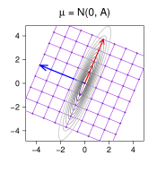
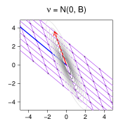
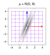
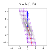
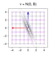
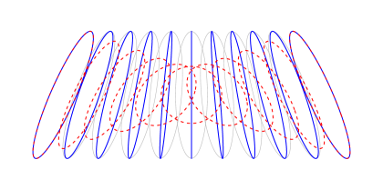
The Wasserstein transport $Y=T_{\mathrm{W}}^{\mu,\nu}X$ is visualized in the top row of Figure 1. Since $\operatorname{diag}(L^{\top}M)=(-3,1)$ contains a negative entry, the Knothe-Rosenblatt coupling is not $\mathcal{AW}_{2}$-optimal. The second row of Figure 1 visualizes the transports $Y=T_{\mathrm{KR}}^{\mu,\nu}X$ and $Y=T_{\mathrm{AW}}^{\mu,\nu}X$ (the later is unique and deterministic by Corollary 4.4). Here we have $\mathcal{W}_{2}(\mu,\nu)\approx 1.75$, $\mathcal{KR}_{2}(\mu,\nu)=4$ and $\mathcal{AW}_{2}(\mu,\nu)=2$ (which is consistent with (5.3)). Note that when $N=2$ all distributions are Markovian. So the Knothe-Rosenblatt coupling is not necessarily optimal even for Gauss-Markov processes. We also visualize, in Figure 2, the interpolations (5.2) based on $T_{\mathrm{W}}^{\mu,\nu}$, $T_{\mathrm{KR}}^{\mu,\nu}$ and $T_{\mathrm{AW}}^{\mu,\nu}$.

Figure 1. Transports between $\mu=\mathcal{N}(0,A)$ and $\nu=\mathcal{N}(0,B)$ where $A$ and $B$ are given by (6.1). Each distribution is visualized by the elliptical contours of its density. Top row: The $\mathcal{W}_{2}$-transport. Here the arrows and the grid correspond to the eigenvectors of $A$. The image of the grid under $T_{\mathrm{W}}^{\mu,\nu}$ is shown on the right. Second row: Now the arrows and the grid correspond to the standard Euclidean basis $\{\mathbf{e}_{1},\mathbf{e}_{2}\}$ in the source space. The middle plot shows the transport under $T_{\mathrm{KR}}^{\mu,\nu}$ and the right plot shows the transport under $T_{\mathrm{AW}}^{\mu,\nu}$. Since $T_{\mathrm{KR}}^{\mu,\nu}$ is comonotonic at each time, $T_{\mathrm{KR}}^{\mu,\nu}\mathbf{e}_{1}$ points towards the right and $T_{\mathrm{KR}}^{\mu,\nu}\mathbf{e}_{2}$ points upward. Here only $T_{\mathrm{ABW}}^{\mu,\nu}\mathbf{e}_{2}$ points upward.

Figure 2. Three interpolations $(A_{t})_{0\leq t\leq 1}$ between $A_{0}=A$ and $A_{1}=B$ as in (6.1). For visualization purposes we also include a uniform translation. The thin (grey) ellipses visualize McCann’s displacement interpolation. The thick dashed (red) ones show the Knothe-Rosenblatt interpolation where $T=L_{1}L_{0}^{-1}$. The thick solid (blue) ones show the interpolation with $T=L_{1}PL_{0}^{-1}$; in this case $A_{\frac{1}{2}}$ is degenerate.

Next we show an example where the optimal $\mathcal{AW}_{2}$-coupling is not unique.

Example 6.3.

Consider

(6.2) $$L=\begin{bmatrix}1&0\\ 1&1\end{bmatrix}\Rightarrow A=\begin{bmatrix}1&1\\ 1&2\end{bmatrix}\quad\text{and}\quad M=\begin{bmatrix}1&0\\ -1&1\end{bmatrix}\Rightarrow B=\begin{bmatrix}1&-1\\ -1&2\end{bmatrix}.$$

Then $\operatorname{diag}(L^{\top}M)=(0,1)$. Thus any optimal $\mathcal{AW}_{2}$-coupling is comonotonic at time $2$ but is otherwise unrestricted. To see intuitively why, use (6.2) to write

$$X_{2}=X_{1}+\epsilon_{2},\quad Y_{1}=-Y_{1}+\epsilon_{2},$$

where $\epsilon_{2}=\epsilon_{2}^{X}=\epsilon_{2}^{Y}\sim\mathcal{N}(0,1)$ is the common noise at time $2$. Since

$$\|X-Y\|^{2}=(X_{1}-Y_{1})^{2}+(X_{2}-Y_{2})^{2}=(X_{1}-Y_{1})^{2}+(X_{1}+Y_{1})^{2},$$

the cross terms cancel out. Thus the transport cost does not depend on the coupling at time $1$.

7. Conclusion

In this paper we derived explicitly the adapted Wasserstein distance between non-degenerate Gaussian distributions and characterized the optimal couplings. Apart from a deeper study of the adapted Wasserstein geometry Gaussian distributions, we may consider the adapted Wasserstein barycenter and entropic regularization of (2.6) with Gaussian marginals. Motivated by the Wasserstein setting [1, 17], it seems natural to conjecture that the solutions to both problems are Gaussian. It is also of interest to use the explicit formula of $d_{\mathrm{ABW}}$ to study, in the spirit of [16], distributionally robust optimization problems under Gaussian dynamics. Finally, our results may be useful for studying the adapted Wasserstein distance between continuous time Gaussian processes which are not necessarily semimartingales.

References

• [1] M. Agueh and G. Carlier. Barycenters in the Wasserstein space. SIAM Journal on Mathematical Analysis, 43(2):904–924, 2011.
• [2] S. Akbari, L. Ganassali, and N. Kiyavash. Causal discovery via monotone triangular transport maps. In NeurIPS 2023 Workshop Optimal Transport and Machine Learning, 2023.
• [3] J. Backhoff-Veraguas, D. Bartl, M. Beiglböck, and M. Eder. All adapted topologies are equal. Probability Theory and Related Fields, 178:1125–1172, 2020.
• [4] J. Backhoff-Veraguas, D. Bartl, M. Beiglböck, and J. Wiesel. Estimating processes in adapted Wasserstein distance. The Annals of Applied Probability, 32(1):529–550, 2022.
• [5] J. Backhoff-Veraguas, M. Beiglböck, M. Eder, and A. Pichler. Fundamental properties of process distances. Stochastic Processes and their Applications, 130(9):5575–5591, 2020.
• [6] J. Backhoff-Veraguas, M. Beiglbock, Y. Lin, and A. Zalashko. Causal transport in discrete time and applications. SIAM Journal on Optimization, 27(4):2528–2562, 2017.
• [7] J. Backhoff-Veraguas, S. Källblad, and B. A. Robinson. Adapted Wasserstein distance between the laws of SDEs. arXiv preprint arXiv:2209.03243, 2022.
• [8] R. Baptista, Y. Marzouk, and O. Zahm. On the representation and learning of monotone triangular transport maps. Foundations of Computational Mathematics, pages 1–46, 2023.
• [9] D. Bartl, M. Beiglböck, and G. Pammer. The Wasserstein space of stochastic processes. arXiv preprint arXiv:2104.14245, 2021.
• [10] M. Beiglböck, G. Pammer, and A. Posch. The Knothe-Rosenblatt distance and its induced topology. arXiv preprint arXiv:2312.16515, 2023.
• [11] R. Bhatia, T. Jain, and Y. Lim. On the Bures–Wasserstein distance between positive definite matrices. Expositiones Mathematicae, 37(2):165–191, 2019.
• [12] J. Bion-Nadal and D. Talay. On a Wasserstein-type distance between solutions to stochastic differential equations. The Annals of Applied Probability, 29(3):1609–1639, 2019.
• [13] S. Cambanis, S. Huang, and G. Simons. On the theory of elliptically contoured distributions. Journal of Multivariate Analysis, 11(3):368–385, 1981.
• [14] S. Eckstein and G. Pammer. Computational methods for adapted optimal transport. The Annals of Applied Probability, 34(1A):675–713, 2024.
• [15] M. Gelbrich. On a formula for the L2superscript𝐿2L^{2} Wasserstein metric between measures on Euclidean and Hilbert spaces. Mathematische Nachrichten, 147(1):185–203, 1990.
• [16] B. Han. Distributionally robust Kalman filtering with volatility uncertainty. arXiv preprint arXiv:2302.05993, 2023.
• [17] H. Janati, B. Muzellec, G. Peyré, and M. Cuturi. Entropic optimal transport between unbalanced Gaussian measures has a closed form. Advances in Neural Information Processing Systems, 33:10468–10479, 2020.
• [18] R. Lassalle. Causal transport plans and their Monge–Kantorovich problems. Stochastic Analysis and Applications, 36(3):452–484, 2018.
• [19] Z. Lin. Riemannian geometry of symmetric positive definite matrices via Cholesky decomposition. SIAM Journal on Matrix Analysis and Applications, 40(4):1353–1370, 2019.
• [20] L. Malagò, L. Montrucchio, and G. Pistone. Wasserstein Riemannian geometry of Gaussian densities. Information Geometry, 1:137–179, 2018.
• [21] R. J. McCann. A convexity principle for interacting gases. Advances in Mathematics, 128(1):153–179, 1997.
• [22] R. J. Muirhead. Aspects of Multivariate Statistical Theory. John Wiley & Sons, 1982.
• [23] F. Otto. The geometry of dissipative evolution equations: the porous medium equation. Communications in Partial Differential Equations, 26:101–174, 2001.
• [24] G. Pammer. A note on the adapted weak topology in discrete time. Electronic Communications in Probability, 29:1–13, 2024.
• [25] B. A. Robinson and M. Szölgyenyi. Bicausal optimal transport for SDEs with irregular coefficients. arXiv preprint arXiv:2403.09941, 2024.
• [26] L. Rüschendorf. The Wasserstein distance and approximation theorems. Probability Theory and Related Fields, 70(1):117–129, 1985.
• [27] A. Takatsu. Wasserstein geometry of Gaussian measures. Osaka Journal of Mathematics, 48(4):1005–1026, 2011.
• [28] M. Zorzi. Optimal transport between Gaussian stationary processes. IEEE Transactions on Automatic Control, 66(10):4939–4944, 2020.