Smooth Actual EIRP Control for EMF Compliance
with Minimum Traffic Guarantees

Abstract

To mitigate Electromagnetic Fields (EMF) human exposure from base stations, international standards bodies define EMF emission requirements that can be translated into limits on the “actual” Equivalent Isotropic Radiated Power (EIRP), i.e., averaged over a sliding time window. We aim to enable base stations to adhere to these constraints while mitigating any impact on user performance. Specifically, our objectives are to: i) ensure compliance with actual EIRP control methods defined in IEC 62232:2022, ii) guarantee a minimum EIRP level, and iii) prevent resource shortages at all times. Initially, we present exact and conservative algorithms to compute the set of feasible EIRP consumption values that fulfill constraints i) and ii) at any given time, referred to as the actual EIRP “budget”. Subsequently, we design a control method based on Drift-Plus-Penalty theory that preemptively curbs EIRP consumption only when needed to avoid future resource shortages.

I Introduction

The Radio Frequency (RF) Electromagnetic Field (EMF) limits for human exposure are established by international bodies in [1], [2]. Considering the variability of EMF emissions from base stations (BTS), the “actual maximum approach” described in [3] provides methods for assessing EMF compliance using time averaged, also called actual, EMF emission values. These include the Equivalent Isotropic Radiated Power (EIRP), that can be controlled during BTS operations. According to channel modeling studies, setting a threshold on the actual EIRP at four times below the maximum value has a minimal impact on end-user performance [4]. However, lower thresholds may be necessary when employing higher directivity antennas [5]. Among the existing approaches for actual EMF emission control, [6] proposes a proportional-differentiating power control procedure that limits the usable bandwidth, while [7] optimizes precoding for MIMO systems by assuming full channel knowledge.

In this paper we propose an actual EIRP control method that complies with [3]. Our approach aims to minimize the impact on user performance by guaranteeing a minimum EIRP level and preemptively reducing emissions to prevent resource shortages. While presented for EIRP control, our method can be adapted to limit any function of the emitted power.

II Problem formulation

The EIRP emitted by an antenna in the azimuth/elevation direction $(\phi,\theta)$ is the product of the radiated power $P$ and the antenna gain $G(\phi,\theta)$:

$$\mathrm{EIRP}(\phi,\theta):=P\,G(\phi,\theta).$$ (1)

In free-space, the power density $S$ measured at distance $R$ from the antenna is proportional to the EIRP:

$$S(\phi,\theta)=\frac{\mathrm{EIRP}(\phi,\theta)}{4\pi R^{2}}\ \ [\mathrm{W}/\mathrm{m}^{2}].$$ (2)

We consider a discrete time grid indexed by $t$ and we denote the EIRP consumption $c_{t}$ as the maximum EIRP over a predefined set of azimuth/elevation angles $\mathcal{A}$, called segment:

$$c_{t}:=\max_{(\phi,\theta)\in\mathcal{A}}\langle\mathrm{EIRP}(\phi,\theta)\rangle_{t}$$ (3)

where $\langle.\rangle_{t}$ averages the EIRP over period $t$. Following [3], the actual EIRP consumption, averaged over a sliding window of $W$ periods, shall not exceed the configured threshold $\overline{C}$:

$$\frac{1}{W}\sum_{i=t-\min(t,W-1)}^{t}\!\!\!c_{i}(\gamma_{i})\leq\overline{C},\qquad\forall\,t\geq 0$$ (4)

where consumption $c_{t}$ is capped by the control variable $\gamma_{t}$:

$$0\leq c_{t}(\gamma_{t})\leq\gamma_{t},\qquad\forall\,t\geq 0.$$ (5)

To enforce (5), various methods can be used, such as reducing the antenna transmit power [8], the transmission bandwidth [6], or the beamforming gain [7]. Our solution, controlling $\gamma$, is agnostic to the specific power limitation method chosen.

To guarantee a minimum service level, we aim to keep the control $\gamma$ above the minimum EIRP level $\rho\overline{C}$:

$$\gamma_{t}\geq\rho\overline{C},\qquad\forall\,t\geq 0.$$ (6)

where $\rho\in[0,1]$. Fulfilling (6) is crucial especially in the presence of Guaranteed Bit-Rate (GBR) traffic.

As it turns out, various control policies can jointly fulfill the constraints (4),(6). The simplest one is a greedy policy that at each period $t$ sets $\gamma_{t}$ to the actual EIRP budget $\Gamma_{t}$, being the highest possible consumption such that (4),(6) can be satisfied.

Such greedy policy is optimal in case of low traffic, where $c_{t}\ll\gamma_{t}$. In this case, the only effect of preemptively curbing consumption to a value $\gamma_{t}<\Gamma_{t}$ is an increase of the transmission delay. Instead, under the high traffic regime, setting $\gamma_{t}=\Gamma_{t}$ leads to budget depletion, after which the control drops to its minimum value $\rho\overline{C}$. One natural method to avoid such drops is to increase $\rho$. Yet, this leads to overly conservative policies: for instance, we observe that when $\rho$ approaches 1, $\Gamma_{t}$ tends to the actual EIRP threshold $\overline{C}$.

Thus, we study a method which decides whether and when preemptively curbing consumption to a value $\gamma_{t}<\Gamma_{t}$ to avoid any future budget depletion. We formalize the desired preemptive control behavior as the one maximizing the average $\alpha$-fairness [9] of the control $\gamma$ over time, where the $\alpha$-fair function is defined as:

$$f(x):=\left\{\begin{array}[]{ll}\frac{x^{1-\alpha}}{1-\alpha}\quad\mathrm{if\ }\alpha\geq 0,\,\alpha\neq 1\\ \log(x)\quad\mathrm{if\ }\alpha=1\end{array}\right..$$ (7)

Hence, our problem becomes:

$$\max_{\gamma} \,\lim_{T\rightarrow\infty}\frac{1}{T}\sum_{t=0}^{T-1}\mathbb{E}\left[f(\gamma_{t})\right]$$ (8)

$$\mathrm{s.t.} \,\eqref{eq:cap},\eqref{eq:EMFconstr},\eqref{eq:rhoC}$$

where the expectation $\mathbb{E}$ is with respect to the user demand.

Note that, if $\alpha=1$, $\alpha$-fairness coincides with proportional fairness; as $\alpha$ grows, it tends to max-min fairness. Since $f(.)$ is concave, small values of $\gamma$ are severely penalized, thus encouraging $\gamma$ to evolve smoothly over time. At the same time, since $f(.)$ is increasing, higher values of the control are preferred. Hence, the policy solving the problem (8) shall preemptively curb the EIRP consumption only “when needed”.

III Actual EIRP budget

We start tackling our EIRP control problem (8) by characterizing its feasibility set, i.e., the set of control values $\gamma$ for which constraints (4)-(6) are fulfilled.

Proposition 1.

Define the variable $\Omega_{t}$ as:

$$\Omega_{t}:=\max_{0\leq k\leq\min(t,W-1)}\sum_{i=1}^{k}\left(c_{t-i}-\rho\overline{C}\right).$$ (9)

To fulfill constraints (4)-(6), $\gamma_{t}$ must satisfy:

$$\rho\overline{C}\leq\gamma_{t}\leq\rho\overline{C}+\overline{C}(1-\rho)W-\Omega_{t}:=\Gamma_{t},\quad\forall\,t\geq 0.$$ (10)

We refer to the upper bound $\Gamma_{t}$ of the feasibility set as budget. All proofs can be found in the Appendix.

III-A Budget computation

We now study how to compute the term $\Omega_{t}$, defining the budget $\Gamma_{t}$ via (10). A naive approach would compute all $W$ terms in (9) and take their maximum. Its complexity is quadratic in the window length $W$, which may be prohibitive in practice, where typically $W\approx 10^{3}$ and the period duration is a few hundreds of ms. Thus, we next design more efficient methods. First, we define the auxiliary variable:

$$\Omega_{t}^{n}:=\,\max_{k=0,\dots,n}\sum_{i=1}^{k}(c_{t-i}-\rho\overline{C}),\quad 0\leq n\leq t,\ \forall\,t\geq 0$$ (11)

and we call $\ell_{t}^{n}$ the argument of the maximum in (11). Note that $\Omega_{t}:=\Omega_{t}^{\min(t,W-1)}$ and $\ell_{t}:=\ell_{t}^{\min(t,W-1)}$, where $\ell_{t}$ is the argument of maximum in (9). We next prove a useful recursive property for $\Omega_{t}^{n}$, where $[.]^{+}:=\max(.,0)$.

Proposition 2.

The following recursive relation holds:

$$\Omega_{t+1}^{n+1}=\,\left[\Omega_{t}^{n}+c_{t}-\rho\overline{C}\right]^{+},\quad n\leq t,\ \forall\,t\geq 0.$$ (12)

Proposition 2 suggests that, in order to compute $\Omega_{t}$, one can apply (12) recursively over the last $W-1$ EIRP consumption samples, as described in Algorithm 1. The computational complexity of such procedure is linear in $W$.

Algorithm 1 From-scratch computation of exact budget $\Gamma_{t}$

Fix period $t$. Initialize $\Omega_{t}:=0$.
for $i=\min(t,W-1),\dots,1$:

• Update $\Omega_{t}:=\left[\Omega_{t}+c_{t-i}-\rho\overline{C}\right]^{+}$

return $\Gamma_{t}=\rho\overline{C}+\overline{C}(1-\rho)W-\Omega_{t}$

III-B Iterative computation

Algorithm 1 computes $\Omega_{t}$ from scratch at each period $t$, i.e., it does not reuse computations performed at previous periods. Yet, under some conditions, $\Omega_{t+1}$ can be computed from $\Omega_{t}$ with constant (and negligible, in practice) complexity. This hinges on the following properties of variables $\Omega,\ell$.

Property 1.

If $\ell_{t}<W-1$, then

$$\Omega_{t+1}=\left[\Omega_{t}+c_{t}-\rho\overline{C}\right]^{+}.$$ (13)

Property 2.

If $\Omega_{t+1}^{n+1}>0$, then $\ell_{t+1}^{n+1}=\ell_{t}^{n}+1$. Else, $\ell_{t+1}^{n+1}=0$.

Property 3.

If $c_{t-i}\geq\rho\overline{C}$ for $0\leq i\leq W-1$, then

$$\Omega_{t+1}=\Omega_{t}+c_{t}-c_{t-W+1}.$$ (14)

Properties 1-3 suggest that, if the last $W$ consumption samples exceed $\rho\overline{C}$, then $\Omega_{t+1}$ can be updated via (14). Else, if $\ell_{t}<W-1$, then $\Omega_{t+1}$ can be derived as (13). In both cases, the incremental complexity is constant with respect to $W$. Else, if $\ell_{t}=W-1$, then $\Omega_{t+1}$ is computed from scratch via the original Algorithm 1. Finally, the value of $\ell_{t}$ is updated via Property 2. This procedure is formalized in Algorithm 2.

Algorithm 2 Update of exact budget $\Gamma_{t}$

Initialize $\ell_{0}:=0,\,c_{i}:=0,\Omega_{0}:=0\ \forall\,i<0$.
for period $t\geq 0$:

• if $c_{t-i}\geq\rho\overline{C},\ \forall\,i=0,\dots,W-1$ then:

  • Set $\Omega_{t+1}=\Omega_{t}+c_{t}-c_{t-W+1}$

• else if $\ell_{t}<W-1$ then: $\Omega_{t+1}=\left[\Omega_{t}+c_{t}-\rho\overline{C}\right]^{+}$

• else: Compute $\Omega_{t+1}$ via Algorithm 1

• if $\Omega_{t+1}>0$ then: $\ell_{t+1}=\ell_{t}+1$

• else: $\ell_{t+1}=0$

• return $\Gamma_{t}=\rho\overline{C}+\overline{C}(1-\rho)W-\Omega_{t}$

III-C Low-complexity conservative approximation

The worst-case complexity of iterative Algorithm 2 is still linear in $W$, although its average complexity is lower than that of Algorithm 1. The natural question is whether one can do better, especially if computational resources are a bottleneck.

We here propose an alternative iterative method that provides a conservative estimate of the EIRP budget with constant complexity, i.e., not depending on the window length $W$.

First, it is convenient to introduce the variable $\widetilde{\Omega}_{t}$, which is a variant of the original $\Omega_{t}$ defined in (9), and is computed as the sum of the consumption excess with respect to $\rho\overline{C}$ over the sliding window:

$$\widetilde{\Omega}_{t}:=\sum_{i=1}^{\min(t,W-1)}\left[c_{t-1}-\rho\overline{C}\right]^{+}.$$ (15)

The associated feasibility set, analogous to (10), writes:

$$\rho\overline{C}\leq\gamma_{t}\leq\rho\overline{C}+\overline{C}(1-\rho)W-\widetilde{\Omega}_{t}:=\widetilde{\Gamma}_{t},\quad\forall\,t\geq 0.$$ (16)

Then, $\widetilde{\Gamma}_{t}$ represents the maximum feasible control under the assumption that all past consumption values below the minimum guaranteed level $\rho\overline{C}$ are overestimated as $\rho\overline{C}$. Consequently, it is expected that the approximated budget is generally lower than the exact budget, as we formalize next.

Proposition 3.

$\widetilde{\Gamma}_{t}\leq\Gamma_{t}$, for all periods $t\geq 0$.

Thus, this approximate method produces overly conservative policies, reducing EIRP consumption more than necessary.

On the positive side, the budget can be updated at each period via a simple rule with constant complexity, only requiring to add the latest consumption excess and subtracting the one exiting the new sliding window, as formalized in Algorithm 3.

Algorithm 3 Update of conservative budget $\widetilde{\Gamma}_{t}$

Initialize $\widetilde{\Omega}_{0}:=0,\ c_{i}:=0,\ \forall\,i<0$.
for period $t\geq 1$:

• Compute $\widetilde{\Omega}_{t}=\widetilde{\Omega}_{t-1}+\left[c_{t-1}-\rho\overline{C}\right]^{+}-\left[c_{t-W}-\rho\overline{C}\right]^{+}$

• return $\widetilde{\Gamma}_{t}=\rho\overline{C}+\overline{C}(1-\rho)W-\widetilde{\Omega}_{t}$

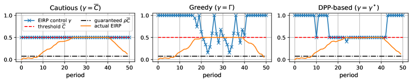
Figure 1: Impact of different control strategies on EIRP consumption under identical input traffic. Parameters: $W=10,\rho=0.15,\alpha=1,\beta=0.95,V=15$.

IV Smooth EIRP control

After characterizing the feasible EIRP control set, we now turn to the solution of the original problem (8).

Two natural strategies arise. One approach is a greedy strategy, where $\gamma_{t}$ is simply set to $\Gamma_{t}$ (or $\gamma_{t}=\widetilde{\Gamma}_{t}$, if the conservative budget is used) for all $t$’s. Here, EIRP is constrained only when necessary. However, under high traffic conditions, the budget can deplete, leading to $\gamma$ being pushed down to its minimum value $\rho\overline{C}$ until the budget refills. Alternatively, to prevent resource shortages, one can cautiously set $\gamma_{t}=\overline{C}$ for all $t$’s. In this case, the control is consistently smooth, but low. While optimal for high-load conditions, this cautious strategy proves overly conservative when traffic is low and EIRP control is unnecessary.

Ideally, the optimal strategy would not restrict EIRP during low traffic, while proactively reducing EIRP as traffic increases or when the budget is limited to prevent future resource shortages. Figure 1 elaborates further on such intuitions.

To effectively control $\gamma$, we propose a method based on Drift-Plus-Penalty (DPP) theory.

IV-A Preliminaries on Drift-Plus-Penalty (DPP)

Drift-Plus-Penalty (DPP) is a stochastic optimization technique typically employed to maximize a network utility while guaranteeing queue stability [10]. Formally speaking, DPP solves problems of the following form:

$$\min_{x_{t}\in A(\omega_{t})} \,\lim_{T\rightarrow\infty}\frac{1}{T}\sum_{t=0}^{T}\mathbb{E}\left[P(x_{t},\omega_{t})\right]:=p^{*}$$ (17)

$$\mathrm{s.t.} \,\lim_{T\rightarrow\infty}\frac{1}{T}\sum_{t=0}^{T-1}\mathbb{E}\left[Y(x_{t},\omega_{t})\right]\leq 0$$ (18)

where $x_{t}$ is the control variable, $\{\omega_{t}\}_{t}$ are i.i.d. random variables, $P,Y$ are deterministic functions and $A(\omega_{t})$ is the feasible control set. By defining the virtual queue $Q$ evolving as $Q_{t+1}=\left[Q_{t}+Y(x_{t},\omega_{t})\right]^{+}$ for all $t\geq 0$, the constraint (18) can be equivalently formulated as $Q$ being mean-rate stable, i.e., $\lim_{t\rightarrow\infty}\mathbb{E}[Q_{t}]/t=0$. The DPP control is computed as:

$$x_{t}^{*}=\operatorname{argmin}_{x\in A(\omega_{t})}Q_{t}Y(x,\omega_{t})+VP(x,\omega_{t})$$ (19)

which jointly reduces the queue Lyapunov drift (defined as the increment $Q_{t+1}^{2}-Q_{t}^{2}$) and the objective function. The parameter $V>0$ regulates the trade-off between the achieved performance, away from the optimal $p^{*}$ by $\mathcal{O}(V)$, and the average size $\mathcal{O}(1/V)$ of the virtual queue, as shown in [10].

IV-B DPP-based heuristic

We can draw a partial parallel between our problem (8) and the DPP formulation (17-18) by setting the control $x_{t}:=\gamma_{t}$, the objective function $P(x_{t},\omega_{t}):=-f(\gamma_{t})$ and the function $Y(x_{t},\omega_{t}):=c_{t}(\gamma_{t})-\overline{C}$. In this case, (19) becomes:

$$\min_{\gamma\in[\rho\overline{C},\Gamma_{t}]}\overline{Q}_{t}c_{t}(\gamma)-Vf^{(\alpha)}(\gamma)$$ (20)

where the virtual queue $\overline{Q}$ evolves as follows:

$$\overline{Q}_{t+1}=\left[\overline{Q}_{t}+c_{t}(\gamma_{t})-\overline{C}\right]^{+},\quad\forall\,t\geq 0$$ (21)

with $\overline{Q}_{0}=0$. Yet, (20) cannot be computed in practice, since $c_{t}(\gamma)$ is an unknown function of $\gamma$. Indeed, the variable $\omega_{t}$ (which can be interpreted as the consumption $c_{t}$ if no power control is applied, i.e., $\gamma_{t}=\infty$) is unknown. We will then bound (20) from above by replacing $c_{t}(\gamma)$ with $\gamma$ via (5) and minimize $\overline{Q}_{t}\gamma-Vf^{(\alpha)}(\gamma)$ instead, leading to the expression:

$$\gamma_{t}^{*}=\min\left(\max\left(V/\overline{Q}_{t}^{1/\alpha},\,\rho\overline{C}\right),\,\Gamma_{t}\right),\quad\forall\,t\geq 0.$$ (22)

Note that, as traffic increases and EIRP consumption consistently surpasses the threshold $\overline{C}$, the virtual queue grows, leading to a decrease in $\gamma$. By preemptively curbing consumption before the budget depletes, we prevent resource scarcity in the future, as illustrated in Figure 1.

A second discrepancy between formulations (8) and (17)-(18) lies in the averaging window, which spans $W$ samples in (8) and has an infinite duration in (17)-(18). It turns out that this leads the virtual queue $\overline{Q}$ to empty at most every $W$ samples in our finite window scenario, as stated below.

Proposition 4.

For any list $\tau=[t^{\prime},\dots,t+W-1]$ of $W$ successive periods, there exists a period $t\in\tau$ where $\overline{Q}_{t}=0$.

As the virtual queue empties, the control $\gamma^{*}_{t}$ as defined in (22) peaks at the budget $\Gamma_{t}$ at most every $W$ samples. This can be particularly problematic in the case of high traffic, where any value $\gamma_{t}>\overline{C}$ results in future budget depletion. To avoid this behavior, we redefine the virtual queue as follows:

$$\overline{Q}^{\beta}_{t+1}=\left[\overline{Q}^{\beta}_{t}+c_{t}(\gamma_{t})-\beta\overline{C}\right]^{+},\quad 0\leq\beta<1,\ \forall\,t\geq 0$$ (23)

where $\beta$ artificially inflates the virtual queue, thus preventing the undesirable behavior demonstrated in Proposition 4. We describe our DPP-based EIRP control method in Algorithm 4.

Algorithm 4 DPP-based power control for EMF compliance

Initialize $\overline{Q}^{\beta}_{0}:=0$.
for period $t\geq 0$:

• Compute the budget $\Gamma_{t}$ via Algorithm 2

• return ${\gamma_{t}^{\beta}}^{*}=\min(\max(V/(\overline{Q}^{\beta}_{t})^{1/\alpha},\,\rho\overline{C}),\,\Gamma_{t})$

• Assess consumption $c_{t}$ and compute $\overline{Q}^{\beta}_{t+1}$ as in (23)

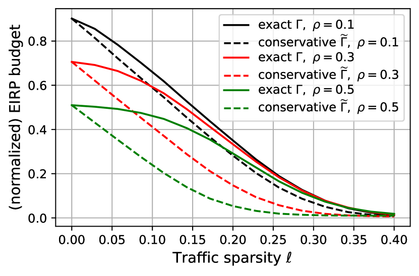
Figure 2: Exact budget $\Gamma$ versus conservative $\widetilde{\Gamma}$ when traffic demands are generated via a sparse zipf distribution that equals 0 with probability $\ell$.

IV-C Numerical evaluations

For our numerical evaluations, we generated a series of traffic demands of $d_{t}$ bits. Demands are sparse: with probability $\ell$, variable $d_{t}$ is drawn from a Zipf distribution, else $d_{t}=0$. The control $\gamma_{t}$ caps the requested EIRP at period $t$. The unserved demand is buffered and shows up again in the next period.

Figure 2 illustrates the relationship between the exact and the conservative budget, $\Gamma$ and $\widetilde{\Gamma}$, respectively. In the case of sparse ($\ell\approx 0$) and high-load ($\ell>0.3$) traffic, the two solutions tend to coincide, as theory suggests. Indeed, as consumption $c$ vanishes, $\Omega$ and $\widetilde{\Omega}$ both tend to zero; conversely, as consumption $c$ increases and is consistently higher than the guaranteed $\rho\overline{C}$, the approximate excess $(c-\rho\overline{C})^{+}$ equals the actual excess $c-\rho\overline{C}$, resulting in an exact budget, i.e., $\widetilde{\Gamma}=\Gamma$. However, in the middle load regime, the exact solution $\Gamma$ outperforms the conservative one $\widetilde{\Gamma}$. In fact, when consumption fluctuates around $\rho\overline{C}$, only the exact solution is able to account for the past “unused” (positive) consumption deficit $\rho\overline{C}-c$ to produce the current budget, while $\widetilde{\Gamma}$ approximates the deficit as null, leading to an overly conservative budget.

Figure 3 illustrates the relationship between the traffic sparsity $\ell$ and the optimal parameter $V$, maximizing the proportional fairness ($\alpha=1$) of the control $\gamma$, as formulated in (8). In the high traffic regime, preemptively curbing emissions becomes necessary to avoid future budget depletion, leading to a decrease in the optimal $V$. Conversely, if the traffic is sparse ($\ell\approx 0$), it is optimal to curb emissions only when the budget depletes, resulting in a higher $V$, and the DPP policy tends towards the greedy one. Since $\beta$ and $V$ have opposite effects on the value of the control $\gamma$, decreasing $\beta$ makes the policy more conservative, leading to an increase in the optimal value of $V$. Here, in practice, one can set $\beta$ to a constant value ($\beta\approx 0.95$) and adjust $V$ according to variations in traffic load.

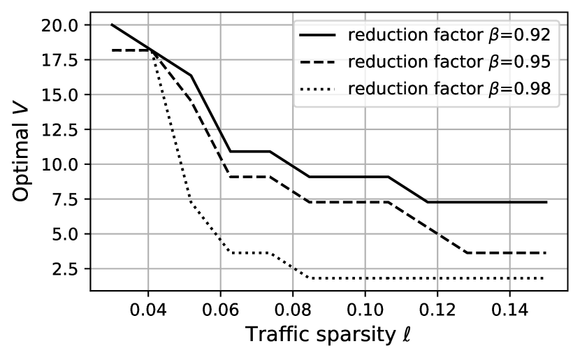
Figure 3: Value of parameter $V$ maximizing proportional fairness as the traffic demand sparsity $\ell$ varies.

V Conclusions

We have investigated an actual EIRP control method designed to ensure compliance with EMF exposure limits established in [1], [2] using the actual maximum approach described in [3]. Our method ensures that the actual EIRP, averaged over a sliding time window, remains below the configured threshold. Additionally, it guarantees a minimum EIRP level at all times, which is crucial for services like GBR traffic. Furthermore, our method proactively limits emissions to prevent future EIRP budget depletion, which could lead to network resource shortages.

To update the EIRP budget over time, we have devised both an exact procedure with linear complexity (Algorithm 2) and a conservative one (Algorithm 3) with constant complexity. Our actual EIRP control algorithm, rooted in Drift-Plus-Penalty theory, preemptively limits EIRP consumption based on the status of a virtual queue, assessing recent consumption overshoot relative to the actual EIRP threshold $\overline{C}$. It relies on one main parameter $V$, which can be adjusted as traffic load profile varies.

Appendix: Proofs

V-A Proposition 1

Proof.

The first inequality in (10) stems from (6). Next we fix period $t$ and assume $\gamma_{t}\leq\Gamma_{t}$. We show that all the constraints (4) containing period $t$ can be satisfied by some control policy. Set $\gamma_{t^{\prime}}=\rho\overline{C}$ for all $t^{\prime}>t$. Then, since $c_{t}\leq\gamma_{t}$,

$$c_{t}\leq\Gamma_{t} =\,\!\!\!\min_{0\leq k\leq W-1}\,\!\!\!W\overline{C}-\!\!\!\sum_{i=1}^{\min(t,k)}\!\!\!c_{t-i}-(W\!-\!k\!-\!1)\rho\overline{C}$$ (24)

$$\leq\,\!\!\!\min_{0\leq k\leq W-1}\!\!\!W\overline{C}-\sum_{i=1}^{\min(t,k)}c_{t-i}-\sum_{i=1}^{W-k-1}c_{t+i}$$ (25)

which is an equivalent expression of all constraints in (4) containing period $t$, Conversely, if $\gamma_{t}>\Gamma_{t}$, then by setting $\gamma_{t^{\prime}}=\rho\overline{C}$ for all $t^{\prime}>t$, at least one constraint (4) is violated if $c_{t^{\prime}}=\gamma_{t^{\prime}}$ for all $t^{\prime}>t$. Then, to satisfy (4) one must set $\gamma_{t^{\prime}}<\rho\overline{C}$ for some $t^{\prime}>t$, which in turn violates constraint (6). Thus, the upper bound is tight, q.e.d.. ∎

V-B Proposition 2

Proof.

We define $a_{t,k}:=\sum_{i=1}^{k}(c_{t-i}-\rho\overline{C})$. By observing that $a_{t+1,k+1}=a_{t,k}+c_{t}-\rho\overline{C}$, we derive that:

$$\Omega_{t+1}^{n+1}=\max_{0\leq k\leq n+1}a_{t+1,k}= \,\max\left(a_{t+1,0},\,\max_{0\leq k\leq n}a_{t+1,k+1}\right)$$

$$= \,\Big{[}\max_{0\leq k\leq n}a_{t,k}+c_{t}-\rho\overline{C}\Big{]}^{+}\!\!\!\!$$ (26)

which equals $\left[\Omega_{t}^{n}+c_{t}-\rho\overline{C}\right]^{+}$, q.e.d.. ∎

V-C Property 1

Proof.

If $t<W-1$, then $\ell_{t}:=\ell_{t}^{\min(t,W-1)}=\ell_{t}^{t}<W-1$. It stems from Proposition 2 that:

$$\Omega_{t+1}^{\min(t+1,W-1)}=\Omega_{t+1}^{t+1}= \,\left[\Omega_{t}^{t}+c_{t}-\rho\overline{C}\right]^{+}$$ (27)

$$= \,\big{[}\Omega_{t}^{\min(t,W-1)}+c_{t}-\rho\overline{C}\big{]}^{+}.$$ (28)

Next, let $t\geq W-1$. From Proposition 2 we know that $\Omega_{t+1}^{W-1}=[\Omega_{t}^{W-2}+c_{t}-\rho\overline{C}]^{+}$. If $\ell_{t}^{W-1}<W-1$, then

$$\Omega_{t}^{W-1}:= \,\max_{0\leq k\leq W-1}a_{t,k}=\,\max_{0\leq k\leq W-2}a_{t,k}=:\,\Omega_{t}^{W-2}.$$ (29)

The thesis follows. ∎

V-D Property 2

Proof.

We define $a_{t,k}$ as in the proof of Proposition 2. Then, $\ell_{t+1}^{n+1}=\operatorname*{arg\,max}_{0\leq k\leq n+1}a_{t+1,k}$. If $\Omega_{t+1}^{n+1}=0$, then $\ell_{t+1}^{n+1}=0$ since $a_{t+1,0}=0$. Else, if $\Omega_{t+1}^{n+1}>0$, we can write:

$$\ell_{t+1}^{n+1}= \,\operatorname*{arg\,max}_{1\leq k\leq n+1}a_{t,k-1}+c_{t}-\rho\overline{C}=\,\operatorname*{arg\,max}_{1\leq k\leq n+1}a_{t,k-1}$$

which equals $\operatorname*{arg\,max}_{0\leq k\leq n}a_{t,k}+1=\ell_{t}^{n}+1$, q.e.d.. ∎

V-E Property 3

Proof.

If $c_{t-i}\geq\rho\overline{C}$ for $0\leq i\leq W-1$, then it stems from (9) that $\Omega_{t}=\sum_{i=1}^{W-1}(c_{t-i}-\rho\overline{C})$ and $\Omega_{t+1}=\sum_{i=0}^{W-2}(c_{t-i}-\rho\overline{C})$. By subtracting term by term we obtain (14), q.e.d.. ∎

V-F Proposition 3

Proof.

Since (16) holds, it suffices to prove that $\Omega_{t}\leq\widetilde{\Omega}_{t}$. Indeed, $\Omega_{t}\leq\max_{0\leq k\leq\min(t,W-1)}\sum_{i=1}^{k}\left[c_{t}-\rho\overline{C}\right]^{+}\!\!=\widetilde{\Omega}_{t}$. ∎

V-G Proposition 4

Proof.

Let $t_{1}:=0<t_{2}<\dots$ be the periods at which $\overline{Q}=0$. Then, we will prove that $t_{i+1}-t_{i}\leq W$ for all $i\geq 0$. Let us suppose that $\overline{Q}_{t_{i}}=0$. We define $\Delta_{i}=\min\{\delta:\,\sum_{j=0}^{\delta}(c_{t_{i}+j}-\overline{C})\leq 0\}$. It stems from (4) that $\Delta_{i}<W$. Also, $\overline{Q}_{t_{i}+\Delta_{i}}=\overline{Q}_{t_{i}}+\sum_{j=0}^{\Delta_{i}-1}(c_{t_{i}+j}-\overline{C})$. Thus,

$$\overline{Q}_{t_{i}+\Delta_{i}+1}= \,\left[\overline{Q}_{t_{i}+\Delta_{i}}+(c_{t_{i}+\Delta_{i}}-\overline{C})\right]^{+}$$ (30)

$$= \,\big{[}\overline{Q}_{t_{i}}+\sum_{j=0}^{\Delta_{i}}(c_{t_{i}+j}-\overline{C})\big{]}^{+}=0.$$ (31)

Therefore, $t_{i+1}-t_{i}=\Delta_{i}+1\leq W$, q.e.d.. ∎

References

- [1] Int. Commission. on Non-Ionizing Radiation Protection (ICNIRP), “Guidelines for limiting exposure to electromagnetic fields (100 kHz to 300 GHz),” Health physics, vol. 118, no. 5, pp. 483–524, 2020.
- [2] IEEE C95. 1-2019, “IEEE standard for safety levels with respect to human exposure to electric, magnetic, and electromagnetic fields, 0 Hz to 300 GHz,” IEEE Std C95. 1-2019 (Revision of IEEE Std C95. 1-2005/Incorporates IEEE Std C95. 1-2019/Cor 1-2019), pp. 1–312, 2019.
- [3] Int. Electrotechnical Commission, “Determination of RF field strength, power density and SAR in the vicinity of radiocommunication base stations for the purpose of evaluating human exposure,” IEC 62232:2022, 2022.
- [4] P. Baracca, A. Weber, T. Wild, and C. Grangeat, “A statistical approach for RF exposure compliance boundary assessment in massive MIMO systems,” in WSA 2018; 22nd International ITG Workshop on Smart Antennas. VDE, 2018, pp. 1–6.
- [5] M. Rybakowski, K. Bechta, C. Grangeat, and P. Kabacik, “Impact of Beamforming Algorithms on the Actual RF EMF Exposure From Massive MIMO Base Stations,” IEEE Access, 2023.
- [6] C. Törnevik, T. Wigren, S. Guo, and K. Huisman, “Time averaged power control of a 4G or a 5G radio base station for RF EMF compliance,” IEEE Access, vol. 8, pp. 211 937–211 950, 2020.
- [7] D. Ying, D. J. Love, and B. M. Hochwald, “Closed-loop precoding and capacity analysis for multiple-antenna wireless systems with user radiation exposure constraints,” IEEE Transactions on Wireless Communications, vol. 14, no. 10, pp. 5859–5870, 2015.
- [8] S. Mandelli, L. Maggi, B. Zheng, C. Grangeat, and A. Zejnilagic, “EMF Exposure Mitigation via MAC Scheduling,” arXiv:2404.06830, 2024.
- [9] J. Mo and J. Walrand, “Fair end-to-end window-based congestion control,” IEEE/ACM Transactions on networking, vol. 8, no. 5, pp. 556–567, 2000.
- [10] M. J. Neely, “Stochastic network optimization with application to communication and queueing systems,” Synthesis Lectures on Communication Networks, vol. 3, no. 1, pp. 1–211, 2010.