The CMS statistical analysis and combination tool: Combine

Abstract

This paper describes the Combine software package used for statistical analyses by the CMS Collaboration. The package, originally designed to perform searches for a Higgs boson and the combined analysis of those searches, has evolved to become the statistical analysis tool presently used in the majority of measurements and searches performed by the CMS Collaboration. It is not specific to the CMS experiment, and this paper is intended to serve as a reference for users outside of the CMS Collaboration, providing an outline of the most salient features and capabilities. Readers are provided with the possibility to run Combine and reproduce examples provided in this paper using a publicly available container image. Since the package is constantly evolving to meet the demands of ever-increasing data sets and analysis sophistication, this paper cannot cover all details of Combine. However, the online documentation referenced within this paper provides an up-to-date and complete user guide.

0.1 Introduction

The CMS statistical analysis software, Combine, is designed with two main features in mind. The first is to provide a command-line interface to several common workflows used in statistical analyses in high-energy physics, and the second is to encapsulate the statistical model using a human-readable configuration file – herein referred to as a “datacard”. These features are intended to ensure consistency in statistical methodology and allow for efficient investigation of potential issues, without limiting the complexity of any single analysis. Perhaps the most important consequence is that the constructed likelihoods can be combined to produce a greater sensitivity in searches or measurements, provided that the data sets are statistically independent. The Combine analysis software is built around the ROOT [1], RooFit [2], and RooStats [2] packages.

The statistical methods in Combine, many of which were developed in the LHC Higgs Combination Group [3], were originally designed for searches for a Higgs boson in proton-proton collisions. The Combine tool was used in early searches [4] for, and the subsequent discovery of, the Higgs boson [5, 6] by the CMS Collaboration. Historically, its main use case within the CMS Collaboration was in searches for the Higgs boson, hence many of the function names and variables used in Combine include “Higgs”. However, the tool is not specific to these searches or measurements of Higgs boson properties but instead is a generic tool usable for various statistical analyses of LHC data. Since the Higgs boson discovery, many extensions have been included that have been used for the statistical analysis in numerous publications of the CMS Collaboration, including measurements of Higgs boson properties [7], searches for supersymmetry [8], and measurements of standard model parameters such as the top quark mass [9]. The Combine tool has also been used with data from the ATLAS and CMS experiments to produce combined measurements of the Higgs boson mass, production and decay rates, and coupling modifiers [10, 11]. Furthermore, the Combine software includes several routines that provide diagnostic information regarding the statistical model and statistical analysis methods used in such publications.

This paper provides a summary of the statistical methods and capabilities of the Combine tool. For complete and up-to-date documentation, it is recommended that the reader consult the online documentation [12].

In this paper, command line instructions are indicated by the symbol $ at the start of the line. Square brackets [option] indicate optional commands that alter the default behavior of Combine, while angular brackets <option value> indicate a value that must be specified by the user. The color scheme for the listings contained in this paper is as follows:

⬇

1Contents of a complete datacard.

⬇

$ Executable command line.

⬇

> Terminal output from the tool.

⬇

Snippet of a datacard or of Python code.

This paper is organized as follows. Section 0.2 details the dependencies of the software and instructions for its installation. The statistical model that is constructed by Combine is described in Section 0.3, followed by detailed explanations of the analysis types available in the tool and instructions on how they are implemented in Section 0.4. Section 0.5 provides instructions on the use of physics models in Combine, with several examples given. This section also provides a concrete example of a full statistical model constructed in Combine. Section 0.6 provides instructions on how to run Combine. It demonstrates several common statistical procedures using the tool, for example, the calculation of maximum likelihood estimates and confidence or credible intervals, and performing goodness of fit tests. Finally, a summary is given in Section 0.7.

0.2 Installation

Aside from ROOT and RooFit, and their dependencies, several additional libraries are used for optimized algebraic calculations, such as vectorization libraries vdt [13], the GNU scientific library gsl [14], and eigen [15]. Additional common libraries are used, which include boost [16], and gzip [17]. The Combine package may be compiled either within a CMS software (cmssw) environment that provides a versioned set of all dependencies, or as a standalone package. Details of different installation instructions are regularly updated in the online documentation. A precompiled version of Combine is available as a Docker [18] container image:

⬇

$ docker run [--platform linux/amd64] --name combine -it gitlab-registry.cern.ch/cms-cloud/combine-standalone:v9.2.0

At the time of writing this paper, the latest version of Combine is v9.2.0, and all of the example datacards and the inputs necessary to run Combine can be found in the tseqdata/tutorials/CAT23001 directory. For statistical calculations that make use of random sampling, the results obtained by a reader are expected to be consistent with, but not identical to, those provided in this paper.

0.3 The statistical model

The primary task of Combine is to produce a statistical model, $p(\text{data};\vec{\Phi})$, which encodes the probability density for the observed data parameterized by the model parameters $\vec{\Phi}$, and is subsequently used for the statistical analysis.

For numerical efficiency, it is useful to factorize the statistical model $p(\text{data};\vec{\Phi})$ as much as possible with respect to both observables and parameters. The parameter space is partitioned into parameters of interest $\vec{\mu}$ and nuisance parameters $\vec{\nu}$. Nuisance parameters are used to model various uncertainties of theoretical and experimental origin, such as those involved in the prediction of process cross sections or associated with luminosity calibration. Furthermore, the observable space is partitioned into primary observables $\vec{x}$, defined as those that appear in components of the model containing the parameters of interest, and auxiliary observables $\vec{y}$ that appear only in components of the model containing nuisance parameters. Each nuisance parameter $\nu_{k}$ (each element of the vector $\vec{\nu}$) is paired with a corresponding auxiliary observable $y_{k}$ (element of $\vec{y}$) in a component of the statistical model that provides information about how well the nuisance parameter is known. Therefore, the statistical model constructed using Combine is factorized into the primary and auxiliary components of the probability as

$$p({\vec{x},\vec{y};\vec{\Phi}})=p(\vec{x};\vec{\mu},\vec{\nu})\prod_{k}p_{k}(y_{k};\nu_{k}),$$ (1)

where $p(\vec{x};\vec{\mu},\vec{\nu})$ is the probability distribution of the observables for the primary analysis, and $p_{k}(y_{k};\nu_{k})$ are the probability distributions of the auxiliary observables. A likelihood function is constructed for a particular data set of independent identically distributed observables $\left\{\vec{x}_{d}\right\}$ as

$$\mathcal{L}(\vec{\Phi})=\prod_{d}p(\vec{x}_{d};\vec{\mu},\vec{\nu})\prod_{k}p_{k}(y_{k};\nu_{k}),$$ (2)

where the subscript $d$ runs over all entries in the data set and the likelihood function is used in both Bayesian and frequentist calculations. Early searches for the Higgs boson by the CMS collaboration reported upper limits on the Higgs boson cross section using both Bayesian and frequentist methods [4] with Combine.

In Combine, the probability density terms associated with the auxiliary observables, $p_{k}(y_{k};\nu_{k})$, can also be reinterpreted as posterior distributions for the nuisance parameters, $p_{k}(\nu_{k}|y_{k})$, resulting from the outcome of measurements of, or otherwise justified constraints on, the auxiliary observables $y_{k}$, through the relationship

$$p_{k}(\nu_{k}|y_{k})\propto p_{k}(y_{k};\nu_{k})\pi_{k}(\nu_{k}),$$ (3)

where $\pi_{k}(\nu_{k})$ are the nuisance parameter priors. This procedure provides probability distributions from which nuisance parameter values can be sampled when generating pseudo-data sets that Combine uses in certain statistical calculations, as described in Section 0.6.3. For all types of nuisance parameters in Combine, the priors are always assumed to be uniform [3] so all of the $\pi_{k}(\nu_{k})$ are constants.

Each element of $\vec{x}$ is referred to as a “channel” and is statistically independent from all other elements of $\vec{x}$. For example, each element of $\vec{x}$ could be the event counts in different reconstructed final states of some data set. The term $p(\vec{x};\vec{\mu},\vec{\nu})$ in Eq. (1) becomes a product over the channels,

$$p(\vec{x};\vec{\mu},\vec{\nu})=\prod_{i}p_{i}({x}_{i};\vec{\mu},\vec{\nu}),$$ (4)

where $i$ runs over the channels that comprise the primary analysis and $p_{i}$ is the probability density function (pdf) for the observable ${x}_{i}$.

The likelihood function constructed by Combine assumes that all $y_{k}$ are statistically independent from each other and from the primary observables. The user must specify the observables and their pdfs using the datacard as described below.

0.4 Supported analysis types

A configuration file in plain text format is required for Combine to define the observables $\vec{x}$ and $\vec{y}$, and their pdfs $p(\vec{x};\vec{\mu},\vec{\nu})$ and $p_{k}(y_{k};\nu_{k})$. This file is the datacard and is the primary input to Combine. The file is also used to specify the observed data needed to define the likelihood function, whether the analysis is a simple counting experiment or a more complex analysis using binned or unbinned distributions of the data with histograms or parametric functions to describe the pdfs.

The package includes a script text2workspace.py that Combine uses to convert the user defined inputs (in the form of the datacard) into a binary representation of the statistical model. The script can be run before running Combine itself to produce a binary ROOT file containing the statistical model in the form of a RooFit RooWorkspace object. The script is automatically run if the datacard is provided as the input to Combine. The script is run with the following command:

⬇

$ text2workspace.py [-m <mass>] [-o <datacard>.root] <datacard>.txt

The output ROOT file is given the same name as the input datacard, with the extension modified to .root unless the option -o is specified. The value of mass, a parameter widely used in searches for new particles, is interpreted by the text2workspace.py script to specify the datacard keyword $MASS, as described in Section 0.4.2.

It is possible to combine several datacards into a single datacard using the combineCards.py script:

⬇

$ combineCards.py Name1=card1.txt Name2=card2.txt .... > <combined card>.txt

This allows for building complex statistical models, while retaining the readability of individual components (datacards) of the model. Multiple instances of any nuisance parameter, sharing the same name, are treated as a single parameter of the statistical model with a single corresponding auxiliary observable $y$, provided that the pdf specified for $y$ is the same in each instance. The rest of this section describes the preparation of datacards and associated inputs for use with Combine.

The first line of the datacard is a declaration of the number of channels, imax, that are present in the statistical model:

⬇

imax <number of channels>

For a single-channel analysis the datacard entry would be imax 1. If the value of imax is specified as “*”, Combine automatically determines the number of channels.

The next lines in the datacard declare the number of processes to be considered, jmax$+1$, and the number of nuisance parameters, kmax:

⬇

jmax <number of processes minus one>

kmax <number of nuisance parameters or sources of systematic uncertainties>

For datacards with a single signal process, jmax is the number of background processes. Datacard lines starting with “#” are ignored by Combine and any amount of whitespace is allowed to separate columns and lines in the datacard. These features can be used to include descriptive comments in the datacard. The next sections of the datacard have a different syntax depending on whether the datacard represents a counting or shape analysis.

0.4.1 Counting analyses

A counting analysis is one for which the statistical model can be cast in the form of Eq. (1) with only one primary observable, namely the total event count in a single channel that includes multiple sources of signal and background. In the following, the primary observable is labeled $n$. The probability to observe $n$ events is described by a Poisson distribution,

$$\mathcal{P}(n;\lambda)=\lambda^{n}\frac{\re^{-\lambda}}{n!},$$ (5)

for which the expected value, $\lambda$, can be a function of one or more parameters, and represents the total number of expected signal and background events.

Each process comes with a specified reference rate and one or more sources of uncertainty that are referred to as “systematic”, even if they are of statistical origin. In Combine the definitions of each systematic uncertainty require the functional form for the probability distribution $p_{k}(y_{k};\nu_{k})$ to be specified. These typically reflect calibration measurements that often result in log-normal or gamma distributions.

Datacard 1 is an example with all of these elements, representing a counting experiment with one channel having a signal process ${\Pp\Pp\mathrm{X}}$ with reference rate of 1.47, two background processes $\PW\PW$ and $\PQt\PAQt$, and three nuisance parameters that model systematic uncertainties in both the signal and background rates. In this example, the integrated luminosity uncertainty (lumi), assumed to be log-normal, results in an uncertainty in the expected signal rate, as well as in the expected rates of the $\PW\PW$ and $\PQt\PAQt$ backgrounds. The reference rates of the signal and background processes are determined using simulation. A log-normal type uncertainty in the signal rate (xs) is included to account for the uncertainty in the predicted cross section of the signal process. A limited number of simulated events are available to determine the rate of the $\PW\PW$ background. The statistical uncertainty due to this limited number of simulated events (nWW) propagates as a gamma distribution to the rate of $\PW\PW$.

The datacard lines immediately following the imax, jmax, and kmax lines describe the number of events observed in each channel. Line number 5, starting with bin, defines the label that should be used for each channel. In this example there is one channel, labeled ch1. Line number 6, starting with the word observation, indicates the number of observed events, which is 0 in Datacard 1. For analyses in which the data are binned in a histogram, a template-based datacard can be used instead of treating each bin of the histogram as a separate channel.

Datacard 1: Counting experiment datacard - datacard-1-counting-experiment.txt

⬇

1imax 1

2jmax 2

3kmax 3

4# A single channel - ch1 - in which 0 events are observed in data

5bin ch1

6observation 0

7# ----------

8bin ch1 ch1 ch1

9process ppX WW tt

10process 0 1 2

11rate 1.47 0.64 0.22

12# ----------

13lumi lnN 1.11 1.11 1.11

14xs lnN 1.20 - -

15nWW gmN 4 - 0.16 -

There are typically several processes that contribute to the overall signal or background expected yields. Lines 8–11 in Datacard 1 describe the number of events expected for each channel and process, arranged in columns. The first column in each row identifies the information expected in the remaining columns. The number of columns beyond the first column must be equal to the total number of processes across all channels, i.e, to the product $\texttt{imax}(\texttt{jmax}+1)$. Line 8 starting with bin indicates that this row specifies the channel that each column refers to. In this case, since there is only a single channel, the number of columns in addition to the first one is equal to the number of signal and background processes in this channel. Lines 9 and 10 starting with process indicate that these rows refer to the labels and types of the various processes. Line 9 provides a label for each process and line 10 defines the type of the process which is either a positive number for a background process, or 0 or a negative number for a signal process. Line 11, starting with rate, indicates the expected event yield in the specified channel and process. This value should be considered as a reference rate for the process, assuming predetermined values for theoretical cross sections, detector acceptance and selection efficiencies, and integrated luminosity of the data set used in the analysis. The rates can be modified by the parameters of the statistical model $\vec{\Phi}$. In the simplest statistical model available in Combine, a single parameter of interest, the signal strength $r$, multiplies the rate of every signal process in the datacard as described in Section 0.5.

The remaining lines 13–15 contain the description of systematic uncertainties that are to be included in the statistical model. Each of these systematic uncertainties is associated with a dedicated nuisance parameter $\nu$. The systematic uncertainties section of the datacard is structured as follows:

• The first column indicates the name used in the binary representation of the statistical model for identifying the uncertainty. This is the name given to the RooFit RooRealVar object that encodes the corresponding nuisance parameter in the statistical model.

• The second column identifies the effect of the associated nuisance parameter and the form of $p(y;\nu)$ to be included in the statistical model. For gamma type nuisance parameters, this column has two entries, which is explained in the following.

• Finally, there are columns describing the effect of the systematic uncertainty on the rate of each process in each channel. The number of columns is the same as for the previous lines declaring channels, processes, and rates. If a process is unaffected by a nuisance parameter, the corresponding column entry for that nuisance parameter is “-”.

The different types of systematic uncertainties that can be included in the datacard for counting experiments are shown in Table 0.4.1. Each of these types results in an associated probability term $p(y;\nu)$ which is either a normal distribution,

$$\mathcal{N}(y;\nu,\sigma_{\nu})=\frac{1}{\sigma_{\nu}\sqrt{2\pi}}\re^{-\frac{1}{2}\left(\frac{\nu-y}{\sigma_{\nu}}\right)^{2}},$$ (6)

Poisson distribution,

$$\mathcal{P}(y;\nu)=\nu^{y}\frac{\re^{-\nu}}{y!},$$ (7)

or uniform distribution,

$$\mathcal{U}(y;a,b)=\begin{cases}\frac{1}{b-a}&\text{if }y\in[a,b],\\ 0&\text{otherwise}.\end{cases}$$ (8)

Equation (6), aside from being used directly for normally distributed observables, is also the building block for log-normally distributed observables, as discussed below. The Poisson distribution of $y$ in Eq. (7) becomes a gamma distribution in $\nu$ when the observed value of $y$ is substituted and the expression is interpreted as a likelihood function.

In Datacard 1 there are three sources of systematic uncertainty that affect one or more processes. Each of these lines results in a single nuisance parameter $\nu$, auxiliary observable $y$, and associated probability density $p(y;\nu)$ being included in the statistical model. The nuisance parameters are $\nu_{\texttt{lumi}},~{}\nu_{\texttt{xs}}$, and $\nu_{\texttt{nWW}}$ with corresponding auxiliary observables $y_{\texttt{lumi}},~{}y_{\texttt{xs}}$, and $y_{\texttt{nWW}}$.

The first two uncertainties are log-normal types [19], detailed below using the integrated luminosity $L$ uncertainty as an example. The rates of signal and background are typically proportional to $L$. The rates defined in the datacard are normalized to a reference value $L_{0}$, which represents the nominal value of the integrated luminosity. Deviations from this reference value are expressed through the dimensionless quantity $f=L/L_{0}$. An estimate $\hat{f}$ is available as a random sample from a pdf $p(\hat{f};f)$. The probability distribution $p(\hat{f};f)$ is log-normal, so that the sampling distribution of $\ln\hat{f}$ is normal, with mean equal to $\ln f$. The standard deviation of $\ln\hat{f}$ can be judiciously written as $\ln\kappa$, where $\kappa$ is a positive constant that is specified in the datacard. The nuisance parameter $\nu$ that controls the systematic uncertainty in the integrated luminosity is then not considered to be $L$ itself, but rather is defined as $\nu=\ln f/\ln\kappa$ from which it follows that the multiplicative factor in the rate corresponding to luminosity is $f(\nu)=\kappa^{\nu}$. The observable $y$ is then a sample from $p(y;\nu)$, which is normal with mean $\nu$ as in Eq. (6), and unity standard deviation. The log-normal type is typically used when $f$ is positive by definition, as is the case with the integrated luminosity, and $p(\hat{f};f)$ continuously approaches zero as $\hat{f}\to 0$.

The first uncertainty in Datacard 1, lumi in line 13, represents the uncertainty in the measured integrated luminosity of the data set. The effect of this uncertainty is 11% on the rate of the ppX, WW, and tt processes. This means that the rates of all three processes are multiplied by a factor of 1.11 when the nuisance parameter $\nu_{\texttt{lumi}}$ is set to $+1$, and by a factor of $1/1.11=0.90$ when it is set to $-1$. The log-normal type is also useful when a systematic uncertainty is taken to be a factor of $\kappa$, also often expressed as percentage uncertainty of $\kappa-1$. This means that high tails of the distribution of $\hat{f}$ above $\kappa f$ and low tails below $f/\kappa$ each contain equal probability of roughly 16%. The second uncertainty in Datacard 1, xs in line 14, represents an uncertainty in the calculation of the theoretical cross section of the signal process. This uncertainty has an effect of 20% on the signal rate while leaving the background processes unaffected.

The gamma type uncertainty is used to model uncertainties in the rate of a particular process due to the limited sample size used to predict the rate. The third uncertainty in Datacard 1, nWW in line 15, is a gamma type uncertainty. This line in the datacard specifies that the reference rate of the WW background process is determined from a sample of 4 simulated events, each with an event weight of 0.16.

Available uncertainty types for counting experiments. The second and third columns indicate the entries for the datacard required to specify the type, and the relative effect on the yield of each process in each channel. The fourth and fifth columns indicate the resulting multiplicative factor by which Combine scales the normalization of the relevant process in the specified channel, and the term $p(y;\nu)$ that is included in Eq. (1). Finally, the last column indicates the default values of $\nu$ and $y$. Where relevant, the value of $\kappa-1$ can be interpreted as the relative uncertainty in the process normalization in a given channel. Uncertainty type Directive Inputs Multiplicative factor, $f(\nu)$ $p(y;\nu)$ Default values Log-normal lnN kappa $\kappa^{\nu}$ $\mathcal{N}(y;\nu,1)$ $\nu=y=0$ Asymmetric log-normal lnN kappaDown, kappaUp $\left(\kappa^{\text{Down}}\right)^{-\nu}$ if $\nu<-0.5$, $\left(\kappa^{\text{Up}}\right)^{\nu}$ if $\nu>0.5$, $\re^{\nu K\left(\kappa^{\text{Down}},\kappa^{\text{Up}},\nu\right)}$ otherwise. $\mathcal{N}(y;\nu,1)$ $\nu=y=0$ Log-uniform lnU kappa $\kappa^{\nu}$ $\mathcal{U}\left(y,1/\kappa,\kappa\right)$ $\nu=y=\frac{1}{2}\left(\kappa+1/\kappa\right)$ Gamma gmN N, alpha $\nu/N$ $\mathcal{P}(y;\nu)$ $\nu=N+1$, $y=N$

The full statistical model that Combine produces by default using Datacard 1 is given in Section 0.5.

0.4.2 Shape analyses

A shape analysis is defined as one that incorporates one or more primary observables, beyond a single number of events, in the statistical model of Eq. (1). The datacard has to be supplemented with two extensions: a new block of lines defining the pdfs for the observables related to each process in each channel, and a block of lines defining systematic uncertainties that affect those pdfs.

The pdf can be parametric or template-based, depending on the inputs provided by the user. In the former case, the parametric pdf for each process has to be provided as a RooFit object that is derived from the RooAbsPdf class. These objects must be contained in a RooWorkspace object that is identified as an input workspace in the datacard. In the latter case, for each channel, histograms must be provided to represent the pdf for each process binned in the observable for that channel. These must be either ROOT TH1 or RooDataHist histogram objects, for analyses in which the data are binned, or RooDataSet objects when the data are unbinned.

As with the counting experiment, the total reference rate of a given process must be identified in the rate line of the datacard. However, there are special options for shape-based analyses:

• A value of -1 in the rate line indicates that Combine should calculate the rate from the input TH1 object using the TH1::Integral method, or the RooDataSet or RooDataHist using the RooAbsData::sumEntries method.

• For parametric shapes defined as RooAbsPdf objects, if a parameter is found in the input workspace with the name pdfname_norm, the rate is multiplied by the value of that parameter.

For shape analyses, the statistical model constructed by Combine is factorized where possible into normalization and shape terms that provide significant gains in computation time. Examples of this factorization can be seen in Eqs. (10) and (17).

Template-based shape analyses

The majority of statistical analyses performed by the CMS Collaboration are template-based analyses. This choice of analysis is particularly common when there is no physically motivated parametric function to describe the pdfs for the primary observables. Example analyses include the observations of Higgs boson decays to bottom quarks [21], which uses the output of a deep neural network, and the production of four top quarks in proton-proton collisions [22], which uses boosted decision trees to construct the observable.

A template-based shape analysis is one in which the observable in each channel is partitioned into $N_{B}$ bins. The number of events $n_{b}$ in the data that fall within each bin $b$ (with $b$ running from 1 to ${N_{B}}$) is considered as an independent Poisson process. The observable $x$ in Eq. (4) in each channel is replaced by the set of observables $n_{b}$ for the purpose of constructing the statistical model in Combine. For each channel, Combine constructs the term $p(x;\vec{\mu},\vec{\nu})$ as a product of Poisson probabilities, yielding

$$p(x;\vec{\mu},\vec{\nu})=\prod_{b=1}^{N_{B}}\mathcal{P}\left({n}_{b};\lambda_{b}(\vec{\mu},\vec{\nu})\right),$$ (9)

where the total expectation for a given bin is denoted as $\lambda_{b}$, and the observed event count in data in a given channel and bin is denoted by $n_{b}$. In the case of $N_{B}=1$, Eq. (9) reduces to the pdf that Combine constructs for a single counting analysis, cf. Eq. (5). For each channel, histograms must be provided that specify, for each bin, the observed data and the expected yield for each process that contributes. These can be provided as either ROOT TH1 objects or RooFit RooDataHist objects. Within each channel, all histograms must use the same partitioning (binning) of the observable. When using RooDataHist objects, the observable name must be the same for all processes within that channel. An explicit check is made to ensure the normalization of the data histogram corresponds to the number of observed events and that the normalization of the histograms matches the rates provided in the datacard in each channel.

Template-based analysis datacards contain one or more rows in the form:

⬇

shapes <process> <channel> <file> <histogram> [<histogram_systematic_uncertainty_variation>]

In this datacard line, process is any of the process names or “*” for all processes, or data_obs for the observed data, and channel is any of the channel names, or “*” for all channels. The value of file gives the name of the ROOT file. The labels histogram and histogram_systematic_uncertainty_variation identify either the names of the TH1 objects or the RooWorkspace and RooDataHist objects within that file. Several keywords in the datacard line are reserved for automatic substitution when constructing the statistical model:

• $PROCESS is substituted with each process label or data_obs for the observed data.

• $CHANNEL is substituted with each channel label.

• $SYSTEMATIC is substituted with the name of each nuisance parameter (with an additional suffix Up or Down) that appears in the lines at the end of the datacard.

• $MASS is replaced with a mass value, which is passed as a command line option.

These lines are interpreted sequentially in the order they appear in the datacard, which allows for multiple instructions with wild card characters and keywords to define the pdfs for each process across the channels. The $MASS keyword was originally intended to allow for a single datacard to be used for different mass hypotheses of the Higgs boson $m_{\PH}$. In analyses such as the search for $\PH\to\PW\PW^{\ast}\to 2\ell 2\PGn$ [23], a different set of histograms for the signal at specific values of $m_{\PH}$ are chosen by specifying this keyword on the command line. In the $\PH\to\PZ\PZ^{\ast}\to 4\ell$ and $\PH\to\PGg\PGg$ analyses, this keyword makes it possible to measure $m_{\PH}$ using the MH parameter, which can be varied continuously [10]. This keyword is useful in searches for new particles whose masses are not known. The Combine package supports arbitrary user-defined keywords in the datacard, the values of which can be set at runtime with the command line. This is particularly useful for analyses in which the probability distributions depend on more than one parameter.

For each channel, the expected value for the total rate in a given bin $b$ is expressed as a sum over processes $p$,

$$\lambda_{b}\left(\vec{\mu},\vec{\nu}\right)=\sum_{p}M_{p}\left(\vec{\mu},\vec{\nu}\right)\omega_{bp}\left(\vec{\nu}\right)+E_{b}\left(\vec{\mu},\vec{\nu}\right),$$ (10)

where the functions $\omega_{bp}(\vec{\nu})$ are the number of expected events for a process in a given bin $b$, $M_{p}\left(\vec{\mu},\vec{\nu}\right)$ is the overall multiplicative factor representing the effects of the statistical model parameters on the total rate of a given process, and $E_{b}(\vec{\mu},\vec{\nu})$, discussed at the end of this section, accounts for the statistical uncertainties arising from limited simulated or collision data used to populate the histogram. The value of $\lambda_{b}\left(\vec{\mu},\vec{\nu}\right)$ is restricted to be positive for any values of the parameters.

The functions $\omega_{bp}(\vec{\nu})$ are derived using the histograms provided by the user that represent the expected distribution for a given process, for the nominal model and for alternates in which a particular nuisance parameter is varied. Dropping the process labels henceforth, the nominal bin contents are denoted by $\omega_{b}^{0}$. For each shape systematic uncertainty $s$, two additional histograms are specified, $\omega_{b}^{s,+}$ and $\omega_{b}^{s,-}$, typically corresponding to the distributions for the values $\nu_{s}=+1$ and $\nu_{s}=-1$, respectively. The datacard must include an additional line in the systematic uncertainties block with the form:

⬇

<name> shape[N] <effect_p_i>

where effect_p_i is a sequence of values that indicate the effect of the uncertainty in each process $p$ and channel $i$ in the datacard. Each value in the sequence can be “-” or 0 for no effect, or 1 to indicate that the process is affected. Values different from 1 can be specified to indicate that the histograms provided represent the expected distribution for other values of the associated nuisance parameter $\nu_{s}$. For example, a value of 0.5 would indicate to Combine that the alternative histograms correspond to values of $\nu_{s}=\pm 2$ as is illustrated for the systematic uncertainty modelled by the nuisance parameter sigma in Datacard 2.

The alternative histograms can be different from the nominal histogram both in the fractional content of each bin, $f_{b}=\omega_{b}/\sum_{b^{\prime}}\omega_{b^{\prime}}$, and in their normalization. For the latter, the term $M_{p}\left(\vec{\mu},\vec{\nu}\right)$ in Eq. (10) contains an additional asymmetric log-normal multiplicative factor, as described in Table 0.4.1, where the values of $\kappa^{\text{Up}}$ and $\kappa^{\text{Down}}$ are defined by

$$\kappa^{\text{Up/Down}}=\frac{\sum_{b}\omega_{b}^{+/-}}{\sum_{b}\omega_{b}^{0}}.$$ (11)

For the former, the user can choose between either parameterizing the variation due to each nuisance parameter directly in terms of the fractional bin contents, $f_{b}$, or their logarithms, $\ln(f_{b})$, by specifying either shape or shapeN in the systematic line of the datacard, respectively. The functions for the fractions are given by

$$f_{b}(\vec{\nu})=f^{0}_{b}+\sum_{s}F(\nu_{s},\delta^{s,+}_{b},\delta^{s,-}_{b},\epsilon_{s}),$$ (12)

if using the shape algorithm or

$$f_{b}(\vec{\nu})=\re^{\left(\ln(f^{0}_{b})+\sum_{s}F(\nu_{s},\Delta^{s,+}_{b},\Delta^{s,-}_{b},\epsilon_{s})\right)},$$ (13)

if using the shapeN algorithm, respectively, where $f^{0}_{b}=\omega^{0}_{b}/\sum_{b^{\prime}}\omega_{b^{\prime}}^{0}$, $\delta^{s,\pm}_{b}=f^{s,\pm}_{b}-f^{0}_{b}$, $\Delta^{s,\pm}_{b}=\ln(f^{s,\pm}_{b})-\ln(f^{0}_{b})$, and the subscript $s$ iterates over each systematic uncertainty. Similarly to the nominal fractions, the values of $f^{s,\pm}_{b}$ are determined by $f^{s,\pm}_{b}=\omega^{s,\pm}_{b}/\sum_{b^{\prime}}\omega^{s,\pm}_{b^{\prime}}$. The shape algorithm is typically used when the variation due to a systematic uncertainty is relatively small compared to the contents in each bin, while the shapeN algorithm is used when a systematic uncertainties results in large variations. This is due to the fact that the latter yields a smooth function close to zero when the fractional bin contents are small.

The function $F$ depends on a set of scaling factors, $\epsilon_{s}$. These are assumed to be unity by default, but may be set to different values, , if the values of $\omega_{b}^{s,\pm}$ correspond to $\nu_{s}=\pm X$, then $\epsilon_{s}=1/X$. The function ${F}$ is defined as

$$F(\nu,\delta^{+},\delta^{-},\epsilon)=\begin{cases}\frac{1}{2}\nu^{\prime}\left((\delta^{+}-\delta^{-})+\frac{1}{8}(\delta^{+}+\delta^{-})J(\overline{\nu})\right),&-q<\nu^{\prime}<q;\\ \nu^{\prime}\delta^{+},&\nu^{\prime}\geq q;\\ -\nu^{\prime}\delta^{-},&\nu^{\prime}\leq-q;\\ \end{cases}$$ (14)

where $\nu^{\prime}=\nu\epsilon$, $\overline{\nu}=\nu^{\prime}/q$, and $J(\overline{\nu})=(3\overline{\nu}^{5}-10\overline{\nu}^{3}+15\overline{\nu})$. The minimum value of $\epsilon$ for a given process in a given channel is $q=\min({{\epsilon_{s}}})$. These functions ensure that the fractions and their first and second derivatives are continuous for all values of $\nu$. A discussion of the different functions that are commonly used for parameterization in template-based analyses can be found in Ref. [24]. For each shape[N] systematic uncertainty line in the datacard corresponding to an uncertainty $s$, an auxiliary observable $y_{s}$ and its probability distribution $p(y_{s};\nu_{s})=\mathcal{N}(y_{s};\nu_{s},1)$ are included in the statistical model in Eq. (1). The default values are $\nu_{s}=y_{s}=0$.

Datacard 2 is an example of a template-based analysis in which the observable $x$ is the output of a multivariate analysis (MVA) discriminator. The histograms defining the distributions of all processes, and their variations due to systematic uncertainties, are contained in a single ROOT file named template-analysis-datacard-input.root. Datacard 2 contains two processes, signal and background.

Datacard 2: Template analysis datacard - datacard-2-template-analysis.txt

⬇

1imax 1

2jmax 1

3kmax 4

4# ---------------

5shapes * * template-analysis-datacard-input.root $PROCESS $PROCESS_$SYSTEMATIC

6# ---------------

7bin ch1

8observation 85

9# ------------------------------

10bin ch1 ch1

11process signal background

12process 0 1

13rate 24 100

14# --------------------------------

15lumi lnN 1.1 1.0

16bgnorm lnN - 1.3

17alpha shape - 1 # uncertainty in the background template.

18sigma shape 0.5 - # uncertainty in the signal template.

Line 5 specifies the mapping between the histograms in the ROOT file (as shown in Table 0.4.2) and the processes defined in the datacard. Lines 17 and 18 provide the definition of systematic uncertainties that affect the probability distribution of the observable for the different processes. In the example, two such uncertainties are listed, one, alpha, that affects only the background process, and the other, sigma, that affects only the signal process. Any text beyond the number of columns expected in these lines is ignored by Combine and can be used to include descriptions of the systematic uncertainties in the datacard. Within the ROOT file, two histograms for each systematic uncertainty are provided, which represent the probability distributions and rates of the signal and background processes when the associated nuisance parameters are varied. In the ROOT file, these are TH1 objects named background_alphaUp and background_alphaDown, and signal_sigmaUp and signal_sigmaDown. Table 0.4.2 shows the TH1 inputs contained in the ROOT file used in Datacard 2.

TH1 objects contained in the template-analysis-datacard-input.root file used in Datacard 2. The histograms used to determine the effects of the sigma parameter on the signal distribution correspond to twice the variation resulting from the systematic uncertainty modelled by the parameter. Object name Description data_obs Histogram containing the observed number of events in each bin of the analysis. signal Histogram containing the expected yields $\omega_{b}^{0}$ of the signal process in each bin of the analysis. background Histogram containing the expected yields $\omega_{b}^{0}$ of the background process in each bin of the analysis. signal_sigmaUp, signal_sigmaDown Histograms containing the expected yields of the signal process for each bin in the analysis when the nuisance parameter sigma is set to $-2$ (Down) $\omega_{b}^{-}$, and $+2$ (Up) $\omega_{b}^{+}$, and all other nuisance parameters are set to their default values. background_alphaUp, background_alphaDown Histograms containing the expected yields of the background process for each bin in the analysis when the nuisance parameter alpha is set to $-1$ (Down) $\omega_{b}^{-}$, and $+1$ (Up) $\omega_{b}^{+}$, and all other nuisance parameters are set to their default values.

Figure 1 shows the histograms used to determine the expected yield $\omega_{b}^{0}$ and yields expected for the variations of the systematic uncertainties $\omega_{b}^{+}$ and $\omega_{b}^{-}$ for the signal and background processes. The histogram for the observed data is also shown.

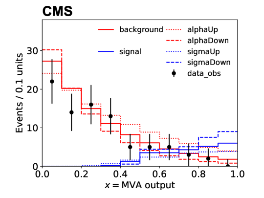
Figure 1: Histograms used to define the pdfs for Datacard 2. The red and blue histograms show the nominal yields in each bin $\omega_{b}^{0}$ for the background and signal processes, respectively. The dotted and dashed lines show the histograms that provide the values of $\omega_{b}^{+}$ and $\omega_{b}^{-}$, respectively for each of the systematic uncertainties that modify the shape of the signal and background pdfs. The red dashed and dotted lines are associated with the effect of the nuisance parameter alpha on the background process, while the blue dashed and dotted lines are associated with the effect of the nuisance parameter sigma affecting the signal process. The black points show the observed number of events in data in each bin. The error bars indicate the statistical uncertainty.

The term $E_{b}\left(\vec{\mu},\vec{\nu}\right)$ in Eq. (10) accounts for the statistical uncertainties in the histograms used to determine $\omega_{bp}$. When the histograms are provided using TH1 objects, these terms can be included using the following line at the end of the datacard:

⬇

<channel> autoMCStats <threshold>

The first string channel should give the name of the channels in the datacard for which these statistical uncertainties should be included. The wildcard “*” indicates that this should apply to all channels in the datacard. The value of threshold should be set to a value greater than or equal to zero to include the uncertainties. This value sets the threshold on the effective number of unweighted events above which the uncertainty is modeled with a single nuisance parameter for each bin following the Barlow–Beeston procedure outlined in Ref. [25], using the simplifying approximation introduced in Ref. [26]. This procedure is used to improve the computational performance without introducing significant impact on the accuracy of the results. Below the threshold, an individual nuisance parameter for each process is created. For each nuisance parameter, a corresponding probability distribution for $y$ is included when building the model in Eq. (1), the form of which is determined by this effective number.

When threshold is set to a number of effective unweighted events greater than or equal to zero, denoted $n^{\text{threshold}}$, the following algorithm is applied to each bin $b$:

1. Sum the yields $\omega^{0}_{bp}$ and uncertainties $e_{bp}$ of each background process $p$ in the bin. $\omega_{\text{tot}}=\sum_{p\,\in\,\text{bkg}}\omega^{0}_{bp}$, and $e_{b,\text{tot}}=\sqrt{\sum_{p\,\in\,\text{bkg}}\,e_{bp}^{2}}$. The values of $e_{bp}$ are obtained using the TH1::GetBinError method.

2. If $e_{b,\text{tot}}=0$, the bin is skipped and no associated nuisance parameters are created.

3. The effective number of unweighted events is defined as $\omega_{b,\text{tot}}^{\text{eff}}=\omega_{b,\text{tot}}^{2}/e_{b,\text{tot}}^{2}$, rounded to the nearest integer.

The value of $\omega_{b,\text{tot}}^{\text{eff}}$ determines the functional form of $E_{b}(\vec{\mu},\nu)$. If $\omega_{b,\text{tot}}^{\text{eff}}>n^{\text{threshold}}$, a single auxiliary observable $y$ is included in the statistical model that is normally distributed with $p(y;\nu)=\mathcal{N}(y;\nu,1)$. The nuisance parameter $\nu$ determines the value of $E_{b}$,

$$E_{b}(\vec{\mu},\vec{\nu},\nu)=\nu\left(\sum_{p}e_{bp}^{2}M_{p}^{2}(\vec{\mu},\vec{\nu})\right)^{\frac{1}{2}},$$ (15)

where $\vec{\nu}$ here represents all of the other nuisance parameters in the statistical model. The default values in Combine are $\nu=y=0$. If instead $\omega_{b,\text{tot}}^{\text{eff}}\leq n^{\text{threshold}}$, a vector of auxiliary observables $\vec{y}$ with one entry per process is included in the statistical model. For processes that have a number of effective events $\omega_{bp}^{2}/e_{pb}^{2}$ less than $n^{\text{threshold}}$, the observable is Poisson distributed with $p(y_{\alpha};\nu_{\alpha})=\mathcal{P}(y_{\alpha};\nu_{\alpha})$. For processes with $w_{bp}^{2}/e_{pb}^{2}\geq n^{\text{threshold}}$, the observable is normally distributed with $p(y_{\beta};\nu_{\beta})=\mathcal{N}(y_{\beta};\nu_{\beta},1)$. The nuisance parameters determine the value of $E_{b}$,

$$E_{b}(\vec{\mu},\vec{\nu},\vec{\nu}_{\alpha},\vec{\nu}_{\beta})=\sum_{\alpha}\left(\frac{\nu_{\alpha}}{y_{\alpha}}-1\right)\omega_{b\alpha}M_{\alpha}(\vec{\mu},\vec{\nu})+\sum_{\beta}\nu_{\beta}e_{b\beta}M_{\beta}(\vec{\mu},\vec{\nu}),$$ (16)

where the indices $\alpha$ and $\beta$ run over processes for which the auxiliary observables are Poisson and normally distributed, respectively. The default values of $\nu_{\beta}=y_{\beta}$ are zero, while the default values of $y_{\alpha}$ and $\nu_{\alpha}$ are set to the effective number of unweighted events in the TH1 histogram objects used to evaluate $\omega_{bp}^{0}$.

Parametric shape analysis

A parametric shape analysis is one that uses analytic functions rather than histograms to describe the pdfs of continuous primary observables. In these cases, the primary observable $x$ in each channel can be univariate or multivariate. For example, in the measurements of Higgs boson cross sections in the four-lepton decay mode, the primary observable is bivariate composed of the invariant mass of the four leptons and a kinematic discriminator designed to separate the signal and background processes [27]. The data in parametric shape analyses can be binned, as in the case of template-based analyses, or unbinned. Uncertainties affecting the expected distributions of the signal and background processes can be implemented directly as uncertainties in the parameters of those analytical functions.

Datacard 3 defines a parametric analysis with a single channel and two processes: one signal process and one background process. The datacard is similar to what would be used in a search for a narrow resonance over a smooth background, such as in the search for Higgs boson decays to muon pairs [28]. The primary observable is the invariant mass $m$ of the decay products, and the signal distribution depends on the hypothesized mass of the resonance, $m_{\PH}$. The systematic uncertainties include uncertainties that affect the expected rates of the signal and background processes, and uncertainties in the parameters that describe the signal and background pdfs.

For datacards describing parametric-based analyses, the term $p(\vec{x};\vec{\mu},\vec{\nu})$ in Eq. (1) is constructed in Combine as,

$$p(\vec{x};\vec{\mu},\vec{\nu})=\sum_{p}\frac{\lambda_{p}(\vec{\mu},\vec{\nu})f_{p}(x;\vec{\mu},\vec{\nu})}{\sum_{p}\lambda_{p}(\vec{\mu},\vec{\nu})},$$ (17)

where $f_{p}(x;\vec{\mu},\vec{\nu})$ are the pdfs for each process $p$ for a given channel with primary observable $x$. These pdfs can depend on both the parameters of interest and the nuisance parameters. In parametric analyses, for a specific data set with $n$ entries $\left\{x_{d}\right\}$ where $d$ runs from 1 to $n$, a Poisson probability $\mathcal{P}\left(n;\sum_{p}\lambda_{p}(\vec{\mu},\vec{\nu})\right)$ is included in the likelihood function in Eq. (2). The Poisson parameters $\lambda_{p}$ depend only on the parameters of interest and any nuisance parameters affecting the rate of a given process. These parameters are products of multiplicative factors of the form given in Table 0.4.1 and any RooAbsReal object named pdfname_norm found in the input RooWorkspace, as described in Section 0.4.2. When the data are provided as binned data sets with RooDataHist objects, the continuous observable $x$ is replaced by a sequence of discrete bin centres $x_{b}$, and the pdfs are evaluated at these values. If the bins are relatively narrow, this approximation provides a good estimate of the probability density. When this approximation is not accurate, the Combine package provides a custom class named RooParametricShapeBinPdf that can wrap any univariate RooAbsPdf object such that

$$f_{p}(x_{b};\vec{\mu},\vec{\nu})=\int_{\text{bin}~{}b}f_{p}(x;\vec{\mu},\vec{\nu})\,\rd{x}.$$ (18)

The datacard lines for parametric shape analyses need two names to identify the RooFit object representing the pdf for a given process in each channel, separated by a colon in the following format:

⬇

shapes <process> <channel> <file> <workspace_name>:<pdf_name>

The label workspace_name identifies the input workspace, which is a RooWorkspace object containing the RooFit objects, while the second label pdf_name identifies the RooAbsPdf or RooAbsData contained therein. The pdfs $f_{p}$ for each process $p$ are defined by the objects identified with pdf_name.

Datacard 3: Parametric analysis datacard - datacard-3-parametric-analysis.txt

⬇

1imax 1

2jmax 1

3kmax 2

4# ---------------

5shapes data_obs bin1 parametric-analysis-datacard-input.root w:data_obs

6shapes signal bin1 parametric-analysis-datacard-input.root w:sig

7shapes background bin1 parametric-analysis-datacard-input.root w:bkg

8# ---------------

9bin bin1

10observation 567

11# ---------------

12bin bin1 bin1

13process signal background

14process 0 1

15rate 10 1

16# ---------------

17lumi lnN 1.1 -

18sigma param 1.0 0.1

19alpha flatParam

20bkg_norm flatParam

Lines 5–7 indicate the name of the input ROOT file parametric-analysis-datacard-input.root that contains an input workspace (w), with RooAbsPdf objects named sig and bkg defining the pdfs for the signal and background processes, respectively. The contents of this workspace are summarized in Table 0.4.2.

Contents of the RooWorkspace object contained in the parametric-analysis-datacard-input.root file providing inputs for the parametric analysis datacard. Object name Type Description m RooRealVar The invariant mass observable. data_obs RooDataSet Invariant mass of each event in the observed data. sig RooGaussian Normal pdf describing the probability distribution of the invariant mass for the signal process. bkg RooExponential Exponential pdf describing the probability distribution of the invariant mass for the background process. MH RooRealVar Mean of the signal pdf. sigma RooRealVar Standard deviation of the signal pdf. alpha RooRealVar Slope parameter for the background pdf. bkg_norm RooRealVar Rate multiplier for the total background contribution.

There is a single RooRealVar object named m in the workspace, which represents the primary observable for the analysis. The RooDataSet object named data_obs provides the observed data. In this datacard the number of events observed in data, as indicated in line 10, is specified as 567, so Combine expects this data set to contain 567 entries, each with its own value of the RooRealVar object m.

Figure 2 shows the pdfs for the signal and background processes, and the distribution of $m$ in observed data. The data are unbinned and treated as such in Combine; the binning is performed exclusively for visualization. The effects of varying the sigma and alpha nuisance parameters on the pdfs for the signal and background processes are also shown.

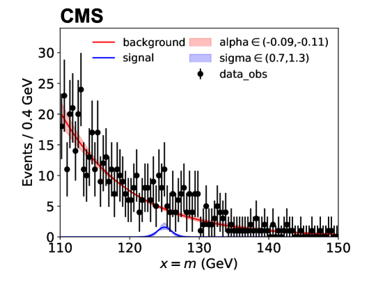
Figure 2: Distributions of the invariant mass observable for the signal and background processes defined in Datacard 3. The red and blue curves show the parametric functions used to define the probability density for the invariant mass for the background and signal processes, respectively, at the default values of the nuisance parameters, normalized to their expected total yields. The blue shaded band shows the variation of the signal pdf when sigma is varied between 0.7 and 1.3. The red shaded region shows the variation of the background pdf when alpha is varied within 10% of its default value of $-0.1$. The black points show the distribution of the observed data. The binning and error bars are only for visualization and neither are used by Combine to build the likelihood function.

In this datacard, the signal process is parameterized as a normal distribution with a mean given by the hypothesized signal mass value MH. This variable is used in Combine when interpreting the command line argument value --mass. The value of the hypothesized signal mass will be fixed to the value specified by the --mass option unless MH is specifically listed as a parameter of interest in the physics model. The background is an exponential distribution $p(m)\propto\re^{\alpha m}$, with a single nuisance parameter defined in the workspace as a RooRealVar object named alpha. The workspace also contains a nuisance parameter named bkg_norm that multiplies the background rate.

Parametric systematic uncertainties are included using datacard lines with the syntax:

⬇

<name> param <V> [<U>, <-UDown/+UUp>]

These datacard lines directly encode uncertainties in the parameters of the signal and background pdfs. For each of these lines, an additional term $\mathcal{N}(y;\nu,u)$, is included when constructing the statistical model in Eq. (1). The default values for $y$ and $\nu$ are set to the value V and $u$ is the value of U specified in the datacard line. Line 18 of Datacard 3 indicates that there is a RooRealVar object describing the parameter sigma, contained in the workspace, that is associated with a normal distribution with mean specified by V$=$1.0 and standard deviation specified by U$=$0.1. Asymmetric uncertainties in the parameter can be defined by using the syntax -UDown/+UUp$=-1/{+}1$ standard deviations in the relevant datacard line. The corresponding term $p(y;\nu)$ in the statistical model constructed by Combine is a dimidated Gaussian distribution [29]. It is possible to include linear correlations between the parameters by first diagonalizing the covariance among them and encoding the resulting linear combinations of parameters as the nuisance parameters that are declared in the datacard.

To specify that a parameter should be assigned a uniform distribution for $p(y;\nu)$, the datacard line should be:

⬇

<name> flatParam

The range of allowed parameter values is determined from the RooRealVar methods getMin and getMax, and the default value of the parameter is determined from the getVal method. Lines 19 and 20 in Datacard 3 indicate that there are two such parameters. These lines do not count towards the value of kmax since for frequentist calculations they can be dropped from the datacard with no effect on the results. The same is not true for Bayesian calculations so it is recommended to include these lines in parametric shape analyses.

0.4.3 Rate parameters

Additional multiplicative scale factors can be introduced in the statistical model that directly modify the rate of a given process, in a given channel, by including additional lines in the datacard for any type of analysis, using the following syntax:

⬇

<name> rateParam <channel> <process> <initial_value> [<min>,<max>]

A nuisance parameter is included in the statistical model that multiplies the rate of that particular process in the given channel by its value. The default value for this parameter is set to the value indicated by initial_value. The values of min and max can be used to set a range for this parameter. The same rateParam nuisance parameter can be attached to multiple channels/processes by using a wild card. For example, “*” matches any process, while “QCD_*” matches any process whose name begins with “QCD_”. Repeating the same datacard line with different channel/process values is also supported. A uniform probability distribution within the range given is included in the statistical model if an additional flatParam datacard line is included for that parameter.

In addition to direct rate modifiers, modifiers that are functions of other parameters can be included using the following syntax:

⬇

<name> rateParam <channel> <process> <formula> <args>

where formula is a string with the syntax used by the ROOT package’s TFormula, and args is a comma separated list of the arguments for the formula. Any nuisance parameter can be included in the formula.

Datacard 4 is an example datacard that uses the rateParam directive to implement an ABCD background estimation method. In the ABCD method, three samples of the data, labeled B, C, and D, that are depleted in signal contributions, are defined using two independent selection variables to estimate one or more background contributions to the signal-enriched data sample labeled A. In Ref. [30], the ABCD method is used to determine the contribution of the QCD multijet background using the missing transverse momentum and an isolation variable based on the measured energy around the electron in each event. The expected contribution from the QCD multijet background in sample A is estimated using the observed yields in samples B, C, and D by assuming the ratio of yields between samples A and B is the same as that between C and D. An example ABCD analysis can be constructed as a four channel counting analysis in Combine, as described in Datacard 4:

Datacard 4: Example ABCD datacard - datacard-4-abcd.txt

⬇

1imax 4

2jmax 1

3kmax *

4# -------

5bin B C D A

6observation 50 100 500 16

7# -------

8bin B C D A A

9process bkg bkg bkg bkg sig

10process 1 2 3 4 0

11rate 1 1 1 1 3

12# -------

13lumi lnN - - - - 1.02

14eff lnN - - - - 1.01

15alpha rateParam A bkg (@0*@1/@2) beta,gamma,delta

16beta rateParam B bkg 50

17gamma rateParam C bkg 100

18delta rateParam D bkg 500

The parameters beta, gamma, and delta described by lines 16–18 are simple rate modifiers, $\beta$, $\gamma$, and $\delta$, that directly scale the yields of the bkg process in channels B, C, and D, respectively. The parameter alpha is determined by the formula $\alpha=\beta\gamma/\delta$, as defined on line 15 of the datacard. The yield of the bkg process in channel A is scaled accordingly by this formula.

Finally, any pre-existing RooAbsReal object inside a ROOT file containing a RooWorkspace can be imported into the statistical model using the following syntax:

⬇

<name> rateParam <channel> <process> <rootfile>:<workspacename>

The value of name should correspond to the name of the RooAbsReal object inside the RooWorkspace. This allows for arbitrary functions of the statistical model parameters to be used to determine the rate of a particular process in a given channel.

0.5 Physics models

The Combine package supports the construction and association of parameters of interest to the different signal processes declared in the datacard. This is achieved by defining the parameters of interest and how they affect the signal processes in a Python file: the physics model. To specify the physics model to use in the statistical model construction, the option -P in text2workspace.py should indicate the Python file and the model defined therein:

⬇

$ text2workspace.py <datacard.txt> -P HiggsAnalysis.CombinedLimit.<PythonFile>:<modelInstance> [--PO <options>]

The PythonFile should be contained in the python/ subdirectory of the Combine package.

The default physics model is one for which the rate of every signal process is multiplied by a common factor $r$, which is the only parameter of interest. In this model $\vec{\mu}=r$. The default model is used if the -P option is not specified.

With the physics model defined, it is now possible to fully determine the statistical model for an input datacard. The statistical model created by Combine for Datacard 1 when using the default physics model is defined as

$$p(n,\vec{y};r,\vec{\nu})=\dfrac{\lambda(r,\vec{\nu})^{n}}{n!}\re^{-\lambda(r,\vec{\nu})}\frac{1}{2\pi}\re^{-\left(\nu_{\texttt{lumi}}-y_{\texttt{lumi}}\right)^{2}}\re^{-\left(\nu_{\texttt{xs}}-y_{\texttt{xs}}\right)^{2}}\frac{\left(\nu_{\texttt{nWW}}\right)^{y_{\texttt{nWW}}}}{y_{\texttt{nWW}}!}\re^{-\nu_{\texttt{nWW}}},$$ (19)

where the function $\lambda(r,\vec{\nu})$ is given by

$$\lambda(r,\vec{\nu})=r\;1.47\;(1.11)^{\nu_{\texttt{lumi}}}(1.2)^{\nu_{\texttt{xs}}}+0.22\;(1.11)^{\nu_{\texttt{lumi}}}+0.64\;(1.11)^{\nu_{\texttt{lumi}}}\frac{\nu_{\texttt{nWW}}}{0.64}.$$ (20)

The observable values for the data are set to $n=0$, $y_{\texttt{lumi}}=y_{\texttt{xs}}=0$, and $y_{\texttt{nWW}}=4$.

Generic physics models can be implemented by writing a Python class that defines the parameters of interest and defines how the signal (and background) yields depend on these parameters. There are numerous example physics models provided in the Combine package in python/PhysicsModel.py and other Python files within the same directory. In the PhysicsModel:floatingXSHiggs physics model, the signal processes expected in the datacard correspond to the four dominant Higgs boson production modes at the LHC: gluon fusion, vector boson fusion, and Higgs boson production associated with a vector boson or a pair of top quarks. Their rates are modified by separate scaling parameters; r_ggH, r_qqH, r_VH (or r_WH and r_ZH), and r_ttH as defined in the following block of code:

⬇

def doParametersOfInterest(self):

"""Create parameters of interest (POIs) and other parameters, and define the POI set."""

# --- Signal Strength as only POI ---

if "ggH" in self.modes: self.modelBuilder.doVar("r_ggH[1,%s,%s]" % (self.ggHRange[0], self.ggHRange[1]))

if "qqH" in self.modes: self.modelBuilder.doVar("r_qqH[1,%s,%s]" % (self.qqHRange[0], self.qqHRange[1]))

if "VH" in self.modes: self.modelBuilder.doVar("r_VH[1,%s,%s]" % (self.VHRange [0], self.VHRange [1]))

if "WH" in self.modes: self.modelBuilder.doVar("r_WH[1,%s,%s]" % (self.WHRange [0], self.WHRange [1]))

if "ZH" in self.modes: self.modelBuilder.doVar("r_ZH[1,%s,%s]" % (self.ZHRange [0], self.ZHRange [1]))

if "ttH" in self.modes: self.modelBuilder.doVar("r_ttH[1,%s,%s]" % (self.ttHRange[0], self.ttHRange[1]))

poi = ",".join(["r_"+m for m in self.modes])

if self.pois: poi = self.pois

...

Each of these is a parameter of interest in the statistical model that Combine constructs. The arrays ggHRange, qqHRange, VHRange, WHRange, ZHRange and ttHRange specify the range of each parameter of interest and are defined in the same Python class. The association of each parameter of interest with each production process is defined in the following function:

⬇

def getHiggsSignalYieldScale(self,production,decay, energy):

if production == "ggH": return ("r_ggH" if "ggH" in self.modes else 1)

if production == "qqH": return ("r_qqH" if "qqH" in self.modes else 1)

if production in [ "WH", "ZH", "VH" ]: return ("r_VH" if "VH" in self.modes else 1)

if production == "ttH": return ("r_ttH" if "ttH" in self.modes else ("r_ggH" if self.ttHasggH else 1))

raise RuntimeError, "Unknown production mode ’%s’" % production

An example datacard with two signal processes and two channels for use with PhysicsModel:floatingXSHiggs is shown in Datacard 5. In this datacard, there are two signal processes, ggH_hgg and qqH_hgg, that correspond to Higgs boson production in the gluon fusion and vector boson fusion modes, respectively, decaying to two photons. The background process is estimated by fitting the data outside the signal peak. The channels correspond to events with an additional pair of jets reconstructed (dijet) or otherwise, leading to a more inclusive channel (incl).

Datacard 5: Multi signal datacard - datacard-5-multi-signal.txt

⬇

1imax 2

2jmax 2

3kmax *

4------------

5shapes * dijet FAKE

6shapes * incl FAKE

7------------

8bin incl dijet

9observation 166 8

10------------

11bin incl incl incl dijet dijet dijet

12process ggH_hgg qqH_hgg bkg ggH_hgg qqH_hgg bkg

13process -1 0 1 -1 0 1

14rate 21 1.6 140 0.4 0.95 3.2

15------------

16QCDscale_ggH lnN 1.12 - - 1.12 - -

17pdf_gg lnN 1.08 - - 1.08 - -

18pdf_qqbar lnN - 1.025 - - 1.025 -

19bg_incl lnN - - 1.05 - - -

The FAKE directive in lines 5 and 6 are used to indicate that each channel of the counting analysis datacard represents a single bin in a histogram. This is required in counting analysis datacards to run some of the diagnostic methods described in Section 0.6.8, and do not change the statistical model constructed by Combine.

It is possible to include generic constraints on the parameters of the physics model. These can be included in the datacard with lines having the following syntax:

⬇

<name> constr <formula> <args> <delta>

where name should be a unique identifier for the constraint and formula and args follow the ROOT TFormula syntax. The result is to multiply the probability term $p(\vec{x};\vec{\mu},\vec{\nu})$ in Eq. (1) by the product of constraint terms,

$$p(\vec{x};\vec{\mu},\vec{\nu})\to p({\vec{x};\vec{\mu},\vec{\nu}})\prod_{l}\frac{1}{\delta_{l}\sqrt{2\pi}}\re^{-\frac{1}{2}\left(\dfrac{g_{l}(\vec{\mu})}{\delta_{l}}\right)^{2}},$$ (21)

where $l$ runs over the constr lines in the datacard. This feature can be used to include additional restrictions on the parameters of the model imposed by external theoretical or experimental constraints. This feature has been used to perform regularization in measurements of unfolded differential Higgs boson cross sections in the $\PH\to\PGt\PGt$ decay mode [31]. As an example, the following datacard line produces a single constraint term in the statistical model with $g(\vec{\mu})=r_{\Pg\Pg\PH}-2r_{\PV\PH}+r_{\PGt\PGt\PH}$ and $\delta=0.03$, when used with the PhysicsModel:floatingXSHiggs physics model:

⬇

constraint_higgs constr @0-2*@2+@1 r_ggH,r_VH,r_ttH 0.03

The order of the list of parameters in the fourth column of the datacard line defines which of the parameters is assigned to each term in $g(\vec{\mu})$.

Throughout this paper, $\mu$ generically denotes the first parameter of interest defined in the physics model, while $r$ specifically refers to the single parameter of interest in the default physics model. For any physics model, it is possible to redefine the list of parameters of interest, or their order within the list, using the Combine command line option --redefineSignalPOIs. Parameters of interest not included in this list are demoted to nuisance parameters. This command may include nuisance parameters, which results in the removal of the probability density in the statistical model for the associated auxiliary observable. This can be used to test how well any parameter of the model can be measured using only the primary observables, and any remaining auxiliary observables of a given data set.

0.6 How to run Combine

This section gives an overview of the command line executable combine provided by the package, which is used to perform a number of different statistical routines using the statistical model constructed by Combine. The executable runs using the command:

⬇

$ combine <datacard.[txt|root]> -M <Method>

Where the Method specifies the statistical calculation to be performed. A list of available options for the executable is displayed by adding the command line option --help.

0.6.1 Generic minimizer options

A number of methods available in Combine make use of numerical optimization of the likelihood function given in Eq. (2). Typically, these methods make use of the profile negative-log-likelihood function, $-\ln{\mathcal{L}(\vec{\mu},\hat{\hat{\vec{\nu}}}(\vec{\mu}))}$, in which the nuisance parameters are profiled; $\hat{\hat{\vec{\nu}}}(\vec{\mu})$ are the values of the nuisance parameters $\nu$ that maximize the likelihood function at a fixed set of values of the parameters of interest $\vec{\mu}$. The class CascadeMinimizer is used to steer these routines and allows for a sequential minimization of $-\ln{\mathcal{L}(\vec{\Phi})}$ using different algorithms. The class also allows for Combine to perform minimization over any discrete nuisance parameters like those needed for the implementation of the discrete profiling method described in Ref. [32]. The combinations of minimizers and algorithms supported in Combine are given in Table 0.6.1. Details of these algorithms can be found in Refs. [14] and [33].

Available combinations of minimizer and algorithms in Combine. Minimizer Reference Available algorithms Minuit [33] Migrad, Simplex, Combined, Scan. Minuit2 [33] Migrad, Simplex, Combined, Scan. GSLMultiMin [14] ConjugateFR, ConjugatePR, BFGS, BFGS2, SteepestDescent.

0.6.2 Output from Combine

Most of the methods available in Combine output the results of the computation to the terminal. In addition these results are also saved in a ROOT file containing a TTree called limit. The name of this file has the following format:

⬇

higgsCombine$NAME.MethodName.mH$MASS.[$WORD$VALUE].root

where NAME is set to the value passed to the option -n, which defaults to Test, and $WORD$VALUE is any user-defined keyword WORD in the datacard that has been set to a particular value VALUE using the command line option --keyword-value WORD=VALUE. The option can be repeated multiple times for multiple keywords. The keyword-value pairs are also stored in the output ROOT file. The option -m sets the value of $MASS and the parameter MH if it is included in the statistical model. Its value is written to the branch mh in the output TTree object.

The structure of the TTree contained in the output ROOT file is given in Table 0.6.2.

TTree branches contained in the output ROOT file from Combine. Branch name Type Description limit Double_t Main result of the statistical routine being performed. limitErr Double_t Estimated uncertainty in the result. mh Double_t Value specified with --mass command line option. The default value is 120. iToy Int_t Pseudo-data set identifier if running with --toys. iSeed Int_t Random seed specified with -s. t_cpu Float_t Estimated processing time. t_real Float_t Elapsed wall-clock time for routine. quantileExpected Float_t Quantile identifier for methods that calculate expected and observed results. The meaning is method-dependent. Negative values are reserved for entries that are not related to quantiles of a calculation. The default is set to $-1$ and specifies that the entry corresponds to the result obtained from the observed data.

0.6.3 Pseudo-data generation

By default, Combine performs the calculation using the observed data. For example, in frequentist methods the observed data are automatically used to construct the likelihood function in Eq. (2). It is possible to run these routines instead using pseudo-data sets to determine the distributions of various statistical quantities such as maximum likelihood estimates, or perform optimization studies that are blind to the observed data.

The option --toys is used to instruct Combine to first generate one or more pseudo-data sets, which are used in place of the observed data. There are two variants of this procedure available in Combine. In the first, specified by --toys <N> with $N>0$, Combine generates $N$ pseudo-data sets from the statistical model and runs the specified statistical routine once per data set. The pseudo-data set is constructed by generating random values of the observables $\vec{x}$. The random number seed for the generation can be modified with the option --seed <value>, which allows the user to ensure each run of the Combine command produces different pseudo-data sets, or identical pseudo-data sets. This allows certain calculations to be split into parallel tasks in the former case and for performing diagnostic studies in particular pseudo-data sets in the latter. The output TTree contains one entry for each of these data sets when generated with $N>0$.

In the second variant, specifying --toys -1 produces an Asimov data set [34]. An Asimov data set is defined as that in which the maximum likelihood estimates for all of the model parameters are equal to the values used to generate the data set. Asimov data sets are used for deriving the expected outcome of frequentist calculations such as in the determination of upper limits and confidence intervals. Where valid, their use makes these calculations much more computationally efficient than using the first variant of pseudo-data generation.

In Combine, Asimov data sets are constructed using the expectation value for the probability $p(\vec{x};\vec{\mu},\vec{\nu})$ in counting analyses and shape analyses for which the data are binned, or by using a large sample of weighted events, which are generated according to $p(\vec{x};\vec{\mu},\vec{\nu})$. The event weights in the latter case are identical for every event in the same channel, and are accounted for when estimating parameter uncertainties from Asimov data sets [35]. The default values of the parameters of interest are used when generating pseudo-data sets in both variants. The command line option --setParameters <x>=<value_x>,<y>=<value_y>,... can be used to specify other values of the parameters to be used for the generation of the pseudo-data sets.

By default, pseudo-data sets in Combine make use of marginalization where the value of each nuisance parameter $\nu_{k}$ is randomly sampled from its probability distribution $p(\nu_{k}|y_{k})$ in Eq. (3) before generating values for the primary observables in each pseudo-data set. The auxiliary observables $\vec{y}$ are set to their default values. This can be modified by specifying the option --toysFrequentist. With this option and $N>0$, a parametric bootstrap [36, 37] is instead performed: each $y$ is generated according to its probability distribution $p(y;\nu)$, where the value of the nuisance parameter $\nu$ is set to the maximum likelihood estimate obtained using the observed data and fixing the parameters of interest to the values specified in the --setParameters option. If instead $N=-1$, the value of $y$ is this maximum likelihood estimate for the corresponding nuisance parameter $\nu$. When specifying the option --bypassFrequentistFit, the default values of the nuisance parameters instead of the maximum likelihood estimates are used.

It is possible to separate the tasks of generating the pseudo-data sets from running statistical routines, by first saving the pseudo-data sets to a ROOT file on disk, and then passing them to any Combine method later. The following sections describe the most commonly used statistical methods available in Combine. These represent only part of the functionality of the tool and users are recommended to consult the online documentation for a full description of its capabilities.

0.6.4 Frequentist limits and confidence intervals

The HybridNew method can be used for calculating upper limits with statistical models created with the default physics model, and for calculating confidence intervals for models with one or more parameters of interest using the Feldman–Cousins procedure [38]. Each of these methods utilizes a test statistic based on the likelihood function given in Eq. (2).

In the case of upper limits, the single parameter of interest $\mu$ corresponds to the parameter $r$ in the default physics model. A number of prescriptions using different test statistics are supported in Combine as follows:

• LEP-style: --testStat LEP --generateNuisances=1 --fitNuisances=0. The test statistic is defined using the ratio of likelihoods,

  $$q_{\mathrm{LEP}}(\mu)=-2\ln\left(\frac{\mathcal{L}(\mu=0,\vec{\nu}_{0})}{\mathcal{L}(\mu,\vec{\nu}_{0})}\right),$$ (22)

  where $\vec{\nu}_{0}$ are the default values of the nuisance parameters. This test statistic was used in the searches for the Higgs boson at the LEP [39].

• TEV-style: --testStat TEV --generateNuisances=0 --generateExternalMeasurements=1 --fitNuisances=1. The test statistic is defined using a ratio of profile likelihoods,

  $$q_{\mathrm{TEV}}(\mu)=-2\ln\left(\frac{\mathcal{L}(\mu=0,\hat{\hat{\vec{\nu}}}(0))}{\mathcal{L}(\mu,\hat{\hat{\vec{\nu}}}({\mu}))}\right),$$ (23)

  where $\hat{\hat{\vec{\nu}}}({0})$, and $\hat{\hat{\vec{\nu}}}({\mu})$ are the values of the nuisance parameters that maximize the likelihood function at $\mu=0$ and $\mu$ respectively. For the purposes of pseudo-data generation, the nuisance parameters are set to the values of $\hat{\hat{\vec{\nu}}}({\mu})$ obtained using the observed data, while the values of $\vec{y}$ are randomly sampled according to their probability densities.

• LHC-style: --LHCmode LHC-limits. The test statistic is defined using a ratio of profile likelihoods,

  $$\widetilde{q}_{\mathrm{LHC}}(\mu)=\begin{cases}-2\ln\left(\dfrac{\mathcal{L}(\mu,\hat{\hat{\vec{\nu}}}({\mu}))}{\mathcal{L}(\hat{\mu},\hat{\vec{\nu}})}\right)&\text{if }0\leq\hat{\mu}\leq{\mu},\\ -2\ln\left(\dfrac{\mathcal{L}(\mu,\hat{\hat{\vec{\nu}}}({\mu}))}{\mathcal{L}(0,\hat{\hat{\vec{\nu}}}(0))}\right)&\text{if }\hat{\mu}<0,\\ 0&\text{if }\hat{\mu}>{\mu},\end{cases}$$ (24)

  where $\hat{\mu}$ is the maximum likelihood estimator for $\mu$. The same result is obtained with the option --testStat LHC --generateNuisances=0 --generateExternalMeasurements=1 --fitNuisances=1. The values of the nuisance parameters $\vec{\nu}$ that maximize the likelihood $\mathcal{L}$ assuming a specific value of $\mu$ and for $\mu=\hat{\mu}$ are denoted $\hat{\hat{\vec{\nu}}}({\mu})$ and $\hat{\vec{\nu}}$, respectively.

The test statistic in Eq. (24) is the most widely used for setting upper limits in searches for new physics at the LHC [3]. In Combine, these test statistics can be modified to perform two point hypothesis tests such as those performed to test different hypotheses for the spin and parity of the Higgs boson [40]. In the LEP-style prescription, the nuisance parameter values for each pseudo-data set are randomly sampled from their distributions $p(\nu_{k}|y_{k})$ in Eq. (3). In the TEV- and LHC-style prescriptions, a parametric bootstrap is used where the nuisance parameters are set to the values of $\hat{\hat{\vec{\nu}}}(\mu)$ obtained using the observed data before generating the primary and auxiliary observables from their probability distributions. It is also possible to integrate out (marginalize) the nuisance parameters in a Bayesian-inspired procedure [41] and advocated for upper limits in high-energy physics analyses [42]. This amounts to calculating

$$\mathcal{L}_{\text{int}}(\vec{\mu})=\int\mathcal{L}(\vec{\Phi})\prod_{k}\pi_{k}(\nu_{k})d\vec{\nu},$$ (25)

where $\mathcal{L}_{\text{int}}(\vec{\mu})$ is the integrated likelihood [41]. In Combine, this is achieved by modifying the options to --generateNuisances=1 and --generateExternalMeasurements=0. This is required to calculate upper limits in cases where there are few or no background events in channels dominated by signal processes such as in the search for lepton flavor violating tau lepton decays performed by the CMS Collaboration [43].

For a specific value of $\mu$, the value of the test statistic using the observed data $q^{\text{obs}}(\mu)$ is calculated, along with the two $p$-values $p_{\mu}$ and $p_{b}$ defined as

$$p_{\mu}=\begin{cases}\int_{q_{\text{x}}^{\text{obs}}(\mu)}^{\infty}f(q_{\text{x}}(\mu)|\mu)\,\rd{q}&\text{if x=LHC},\\ \int_{-\infty}^{q_{\text{x}}^{\text{obs}}(\mu)}f(q_{\text{x}}(\mu)|\mu)\,\rd{q}&\text{if x=TEV or LEP},\end{cases}$$ (26)

and

$$p_{b}=\begin{cases}\int_{0}^{q_{\text{x}}^{\text{obs}}(\mu)}f(q_{\text{x}}(\mu)|0)\,\rd{q_{x}}&\text{if x=LHC},\\ \int_{q_{\text{x}}^{\text{obs}}(\mu)}^{\infty}f(q_{\text{x}}(\mu)|0)\,\rd{q_{x}}&\text{if x=TEV or LEP},\end{cases}$$ (27)

where the distributions of the test statistics $f(q_{\text{x}}(\mu)|\mu)$ and $f(q_{\text{x}}(\mu)|0)$ are determined using pseudo-data sets, assuming the value of $\mu$ indicated and the values of $\vec{\nu}$ and $\vec{y}$ depending on the options used, as described above. From these $p$-values, the tool calculates the criterion [44, 45, 20] defined by $\CLs=p_{\mu}/(1-p_{b})$. The tool then uses a bisection algorithm to find the value of $\mu$ for which $\CLs=\alpha$ corresponding to the upper limit on $\mu$ at the $100(1-\alpha)\%$ confidence level (). The tool can also calculate the median, and 2.5, 16, 85, or 97.5% quantiles of the expected distribution of the upper limit assuming $\mu=0$, by including the option --expectedFromGrid=<X>, where X is either 0.5, 0.025, 0.16, 0.84, or 0.975, respectively.

The 95% upper limit on $\mu$ in the example template analysis can be calculated using Datacard 2 with the command:

⬇

$ combine datacard-2-template-analysis.txt -M HybridNew --LHCmode LHC-limits --rMax 2.0 --clsAcc 0.01

The results of the calculation are output to the terminal as:

⬇

> -- Hybrid New --

> Limit: r < 0.346362 +/- 0.0134581 @ 95% CL

> Done in 0.31 min (cpu), 0.32 min (real)

The bisection algorithm for calculating the upper limit terminates when the estimate of the precision on the upper limit value is below a specified threshold, or when the precision cannot be improved further. The user can specify the following options to control this behavior:

• --rAbsAcc and --rRelAcc: Define the accuracy on the upper limit, $\mu_{\text{up}}$ at which the algorithm terminates. The default values are 0.1 and 0.05 respectively, meaning that the search terminates when the absolute accuracy $\Delta\mu_{\text{up}}<0.1$ or the relative accuracy $\Delta\mu_{\text{up}}/\mu_{\text{up}}<0.05$, where $\Delta\mu_{\text{up}}$ is the estimated uncertainty on the upper limit.

• --clsAcc: Determines the absolute accuracy up to which the value of (or $p_{\mu}$) values are computed when searching for the upper limit. The default is 0.5%.

• -T or --toysH: Determines the minimum number of pseudo-data sets that are generated for each value of $\mu$ with a default value of 500.

The distributions of the test statistic for the pseudo-data sets generated assuming each value of $\mu$ that is tested during the bisection algorithm and $\mu=0$ can be saved in the output file by specifying the option --saveHybridResult. Figure 3 shows the distributions of the test statistic $\widetilde{q}_{\mathrm{LHC}}(\mu=0.4)$ for $\mu=0$ and 0.4 in pseudo-data sets obtained with Datacard 2.

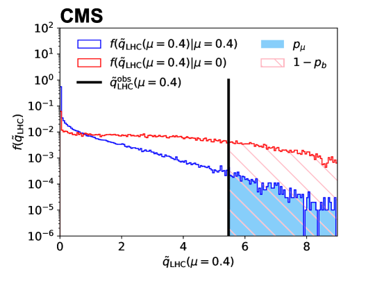
Figure 3: Distributions of $\widetilde{q}_{\mathrm{LHC}}(\mu=0.4)$ from 100,000 pseudo-data sets for $\mu=0$ (red histogram) and $\mu=0.4$ (blue histogram) using the analysis described in Datacard 2. The observed value of the test statistic is indicated by the black vertical line and the regions used to determine $1-p_{b}$ and $p_{\mu}$ are indicated by the pink hatched and light blue shaded regions, respectively.

To further improve the accuracy when searching for the upper limit, Combine interpolates across several results to estimate $\mu_{\text{up}}$. The interpolation uses an exponential function that is fit to the set of results that are closest to the chosen and the range in $\mu$ used for the fit is determined by the accuracy specified in the command line. A plot of the calculated value as a function of $\mu$ can be produced using the option --plot=name.png. Figure 4 shows the calculation of the upper limit at the 95% using the criterion with Datacard 2.

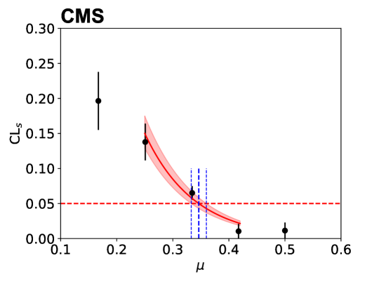
Figure 4: Calculated as a function of $\mu$, used to determine the 95% upper limit for Datacard 2. The solid red line is used to interpolate the values to find the crossing at 0.05, and the shaded band indicates the uncertainty in the interpolation that is used to estimate an uncertainty in the upper limit. The vertical dashed blue lines show the derived upper limit and the estimated uncertainty due to the number of pseudo-data sets used in the calculation.

The AsymptoticLimits method can be used to calculate the upper limits in statistical models that use the default physics model with the LHC-style prescription. This is the default method that will be run if the command line option -M is not specified. In this method, the limit calculation relies on asymptotic approximations for the distributions of the $\widetilde{q}_{\mathrm{LHC}}(\mu)$, following the prescription described in Ref. [34]. The tool also calculates the median and 2.5, 16, 85 and 97.5% quantiles of the expected distribution of the upper limit assuming $\mu=0$, using an Asimov data set. The output TTree contains an entry for each of these results, which can be identified by the quantileExpected branch.

By default upper limits are calculated at the 95% ($\alpha=0.05$). This can be modified using the option --cl=<X> where X is $(1-\alpha)$. Upper limits are calculated using the criterion by default. Alternatively, it is possible to only use $p_{\mu}$ by specifying the option --rule Pmu in the command line. It is also possible to calculate the values of and $p_{\mu}$ for a single value of $\mu$, bypassing the bisection algorithm, by specifying --singlePoint <r>, where r is the desired value of $\mu$.

The HybridNew method can also be used to compute Feldman–Cousins intervals by specifying the option --LHCmode LHC-feldman-cousins. This method allows for calculating confidence intervals with accurate coverage both in scenarios with low event counts or where physical boundaries are placed on the parameters of interest $\mu$. For example, this method has been used in Higgs boson property measurements at CMS [46]. The following procedure can be used to produce one-dimensional confidence intervals or multidimensional confidence regions for physics models with multiple parameters of interest:

• For each parameter point, run the HybridNew method with the option --LHCmode LHC-feldman-cousins --singlePoint <mu1>=<v1>,<mu2>=<v2>,<mu3>=<v3>,... --saveHybridResult to generate the distributions of the test statistic

  $$q_{\mathrm{FC}}(\vec{\mu})=\text{-}2\ln\left(\dfrac{\mathcal{L}(\vec{\mu},\hat{\hat{\vec{\nu}}}({\vec{\mu}}))}{\mathcal{L}_{\Omega}(\hat{\vec{\mu}},\hat{\vec{\nu}})}\right),$$ (28)

  where $\vec{\mu}=\mu_{1},\mu_{2},...$ are the parameters of interest and $\mathcal{L}_{\Omega}(\hat{\vec{\mu}},\hat{\vec{\nu}})$ indicates the maximum of the likelihood function within the bounded region $\Omega$ of its parameters. This region can be defined using the command line option --setParameterRanges <mu1>=<mu1min>,<mu1max>:<mu2>=<mu2min>,<mu2max>:... This step also calculates the value of the test statistic for the observed data $q^{\text{obs}}_{\mathrm{FC}}(\vec{\mu})$.

• Collect the resulting output files into a single ROOT file and find the set of points for which

  $$\int_{q^{\text{obs}}_{\mathrm{FC}}(\vec{\mu})}^{\infty}f(q_{\mathrm{FC}}(\vec{\mu})|\vec{\mu})\,\rd{q_{\mathrm{FC}}}>\alpha,$$ (29)

  to form the $100(1-\alpha)\%$ allowed region.

• The output ROOT file contains the test statistic value for each pseudo-data set as RooFit RooStats::HybridResult objects. These can be used to determine confidence intervals or contours at different values of $\alpha$.

0.6.5 Significance calculation

The HybridNew method is also used to calculate the significance of the observed data when considered against a null hypothesis. For statistical models constructed using the default physics model, this estimates the significance of the presence of a signal contribution in the data where the null hypothesis represents the absence of the signal. By specifying the options --LHCmode LHC-significance, Combine generates pseudo-data under the background-only hypothesis ($\mu=0$) and evaluates the test statistic $q_{0}$ defined by

$$q_{0}=\begin{cases}-2\ln\left(\frac{\mathcal{L}(0,\hat{\hat{\vec{\nu}}}({0}))}{\mathcal{L}(\hat{\mu},\hat{\vec{\nu}})}\right)&\text{if }\hat{\mu}>0\\ 0&\text{otherwise},\end{cases}$$ (30)

for each pseudo-data set. The value of the test statistic for the observed data $q^{\text{obs}}_{0}$ is also calculated in order to determine the $p$-value

$$p_{0}=\int_{q^{\text{obs}}_{0}}^{\infty}f(q_{0}|0)\,\rd{q_{0}},$$ (31)

where $f(q_{0}|0)$ is the distribution of the test statistic determined using the pseudo-data sets. Figure 5 shows the observed value of $q_{0}$ and the distribution of $q_{0}$ in pseudo-data sets assuming $\mu=0$ for Datacard 3.

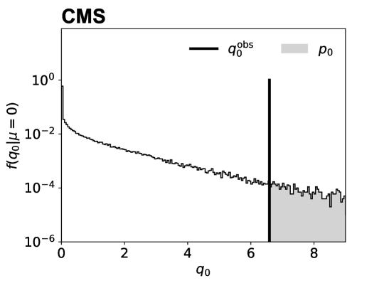
Figure 5: Distribution of $q_{0}$ in 100,000 pseudo-data sets from Datacard 3. The observed value of the test statistic is indicated by the black vertical line and the region used to determine $p_{0}$ is indicated by the light gray shaded region.

The value of $p_{0}$ and corresponding significance of the signal in the example parametric analysis can be calculated using 100,000 pseudo-data sets with Datacard 3 using the command line below:

⬇

$ combine datacard-3-parametric-analysis.txt -M HybridNew --LHCmode LHC-significance -T 100000 --mass 125

The results are output to the terminal as:

⬇

> -- Hybrid New --

> Significance: 2.54397 -0.0146063/+0.0151701

> Null p-value: 0.00548 +/- 0.000233452

> Done in 5.95 min (cpu), 7.57 min (real)

The value of $p_{0}$ is converted into a significance using a standard normal distribution [20]. The method Significance can be used in order to speed up the calculation using the asymptotic approximation for the distribution $f(q_{0}|\mu=0)$ given in Ref. [34] thereby avoiding the need to generate pseudo-data in cases where the number of events in data is large. For the same datacard, the asymptotic approximation for the significance can be calculated with:

⬇

$ combine datacard-3-parametric-analysis.txt -M Significance --mass 125

The result of the calculation using the asymptotic approximation is output to the terminal as:

⬇

> -- Significance --

> Significance: 2.56729

> Done in 0.00 min (cpu), 0.00 min (real)

The significance result and its estimated uncertainty are stored in the output ROOT file in the limit and limitErr branches, respectively. Using the --pval option, the $p$-value is stored instead of the significance.

0.6.6 Bayesian upper limits and credible regions

Bayesian calculations in Combine are based on the posterior probability $p(\vec{\mu})$ defined by

$$p(\vec{\mu})=\frac{1}{p(\left\{\vec{x}\right\}_{d})}\int\mathcal{L}\left(\vec{\Phi}\right)\prod_{k}\pi_{k}(\nu_{k})\rho(\vec{\mu})\,\rd\vec{\nu},$$ (32)

where the index $d$ runs over the events in the observed data set $\left\{\vec{x}\right\}_{d}$, and $p(\left\{\vec{x}\right\}_{d})$ is defined such that $\int p(\vec{\mu})\,\rd\vec{\mu}=1$. The prior term for the parameters of interest $\rho(\vec{\mu})$ must be specified by the user. By default this prior is assumed to be uniform over the ranges $(a_{i},b_{i})$ specified for each parameter of interest $\mu_{i}$,

$$\rho(\vec{\mu})\propto\prod_{i}\mathcal{U}(\mu_{i};a_{i},b_{i}).$$ (33)

Bayesian upper limits are calculated in Combine using either the BayesianSimple method for relatively simple statistical models or the MarkovChainMC method for models with multiple parameters of interest or nuisance parameters, which perform the marginalization over the nuisance parameters. For statistical models with a single parameter of interest $\mu$, the prior can be modified via the command line using the option --prior <prior> with the following options available:

• flat: the default uniform prior.

• 1/sqrt(r): inverse square root prior. This is the Jeffreys prior for the mean of a Poisson distribution [47].

• Any valid ROOT TMath::Formula expression with @0 as the parameter of interest.

• Any string that names a RooFit RooAbsPdf object contained in one of the input workspaces. This option can also be used for statistical models with multiple parameters of interest.

Both methods compute the $100(1-\alpha)\%$ credible upper limit on the parameter of interest $\mu_{\text{up}}$ as

$$\int_{-\infty}^{\mu_{\text{up}}}p(\mu)\,\rd\mu=1-\alpha.$$ (34)

The value of $\alpha$ can be modified by specifying the option --cl=$1-\alpha$.

The BayesianSimple method computes $\mu_{\text{up}}$ using numerical integration, while the MarkovChainMC method uses Markov chain integration [48].

The number of steps in the Markov chain and number of chains to compute can be specified via the command line, as well as the number of steps to ignore from the start of the chain. The user can specify a proposal algorithm by which the Markov chain evolves using the option --proposal <algorithm> with the following options:

• uniform: Selects the next parameter point in the chain at random.

• gaus: Uses a product of independent normal distributions, one for each nuisance parameter where the standard deviation of the distribution for each variable is set to some fraction of the range of the parameter defined by the option --propHelperWidthRangeDivisor.

• ortho: This is the default proposal and is similar to the gaus proposal except that at each point in the chain, only a single parameter is varied.

• fit: With this proposal, Combine computes the Hessian matrix of $-2\ln p(\vec{x};\mu,\vec{\nu})$ with respect to the nuisance parameters $\vec{\nu}$ to construct the proposal function. The accuracy can be improved by including the option --runMinos.

The value of $\mu_{\text{up}}$ and an estimate of its uncertainty are obtained from the average over $N$ independent Markov chains, specified by the command line option --tries <N>. The 95% Bayesian upper limit on the default physics model parameter $r$ for Datacard 1 using 100 Markov chains can be calculated using the following:

⬇

$ combine datacard-1-counting-experiment.txt -M MarkovChainMC --tries 100

These values are saved in the output ROOT file and output to the terminal as below:

⬇

> -- MarkovChainMC --

> Limit: r < 2.21031 +/- 0.0133576 @ 95% credibility (100 tries)

> Done in 0.05 min (cpu), 0.05 min (real)

If using the MarkovChainMC method, it is also possible to store the resulting Markov chains in the output file from Combine using the option --saveChain. This allows for estimating the posterior distribution $p(\vec{\mu})$ for one or more parameters of the model and deriving credible intervals or regions.

0.6.7 Maximum likelihood estimates and scans

Likelihood-based parameter estimation is performed in Combine using the MultiDimFit method. This method can be used to calculate maximum likelihood estimates for the parameter values and their uncertainties through several different approaches. This method has been used by the CMS Collaboration to provide measurements in a number of different scenarios, including Higgs boson production and decay rates, and measurements of the Higgs boson couplings [49]. The MultiDimFit method is used to evaluate the negative-log-likelihood function, ${-}\ln\mathcal{L}(\vec{\Phi})$, and obtain maximum likelihood estimates and estimates of confidence intervals for the parameters of interest $\vec{\mu}$ using the profile likelihood ratio,

$$q(\vec{\mu})=-\ln\left(\frac{\mathcal{L}(\vec{\mu},\hat{\hat{\vec{\nu}}}({\vec{\mu}}))}{\mathcal{L}(\hat{\vec{\mu}},\hat{\vec{\nu}})}\right),$$ (35)

where $\hat{\vec{\mu}}$ are the maximum likelihood estimates for the parameters of interest, and $\hat{\hat{\vec{\nu}}}({\vec{\mu}})$ and $\hat{\vec{\nu}}$ are the values of the nuisance parameters for which $\mathcal{L}$ is maximized for a specific set of parameter values $\vec{\mu}$ and for the maximum likelihood estimates $\hat{\vec{\mu}}$, respectively. The process of finding the parameter values that maximize the likelihood function is typically referred to as a “fit”. In Eq. (35) there are two such fits. The one in the denominator is often referred to as the “overall best fit”. The default parameter values are commonly referred to as “pre-fit”, while the maximum likelihood estimates are commonly referred to as “post-fit”. Throughout this and following sections, the process of determining the maximum likelihood estimates is referred to as maximum likelihood optimization so as not to confuse this procedure with the more general “goodness of fit” methods described in Section 0.6.8.

The following choices for the --algo option are supported in Combine:

• none: this is the default algorithm. The algorithm finds the parameter values $\hat{\vec{\Phi}}$ that maximize $\mathcal{L}(\vec{\Phi})$ and reports the maximum likelihood estimates of the parameters of interest. For a model with $N$ parameters of interest, the output TTree contains $N$ branches, one for each parameter of interest with the maximum likelihood estimates. The output of this algorithm can be used as the starting point for the other algorithms to reduce their evaluation time.

• singles: the algorithm determines the maximum likelihood estimates for each parameter of interest $\mu$ and sequentially determines 68% confidence intervals for each parameter of interest. The output TTree contains one branch for each parameter of interest. One of the entries contains the maximum likelihood estimates with quantileExpected set to $-1$. Two additional entries for each parameter of interest provide the upper $\mu^{+}$ and lower $\mu^{-}$ bounds of the 68% interval for that parameter determined as the range of that parameter for which $q(\mu)<1/2$.

• cross: the algorithm determines the maximum likelihood estimates for each parameter of interest and a set of intervals for each parameter $\mu_{l}$ for which $q(\mu_{l})<\frac{c}{2}$, where $c$ is determined by $\int_{c}^{\infty}\chi^{2}(x;n)\,\rd{x}=\alpha$ and $\chi^{2}(x;n)$ is a chi-squared distribution with the number of degrees of freedom equal to the number of parameters of interest $n$. The output TTree has one entry with the maximum likelihood estimates for the parameters of interest $\hat{\mu}$, and two entries for each parameter of interest, corresponding to the points that define the interval.

• contour2d: for statistical models with two parameters of interest, this algorithm constructs two dimensional contours bounding the regions for which $q(\vec{\mu})<\frac{c}{2}$, where $c$ is computed from $\int_{c}^{\infty}\chi^{2}(x;2)\,\rd{x}=\alpha$. The output contains values corresponding to the maximum likelihood estimates with quantileExpected set to $-1$, and additional entries that define the contour. For $\alpha=0.32$ the contour produced corresponds to $c=2.3$ [20].

• random: in this algorithm, the value of $q(\vec{\mu})$ is evaluated for $N$ uniformly distributed random points in the space spanned by the parameters of interest. The number of points is set by the option --points=<N>.

• fixed: in this algorithm, value of $q(\vec{\mu})$ is calculated at a specified point in the space spanned by the parameters of interest. The fixed point is specified using the --fixedPointPOIs option.

• grid: the value of $q(\vec{\mu})$ is evaluated on a grid of parameter of interest points with $N$ points in total. The number of points $N$ is specified with the option --points=<N>. It is possible to partition the scan into multiple runs of Combine using the options --firstPoint <n> and --lastPoint <m>, where ${0}\leq$n$<$m$\leq N$.

The fixed and grid algorithms can be used to evaluate the likelihood function and $q(\vec{\mu})$ for any value of the statistical model parameters. In each of the above options the value of $\alpha$ can be defined using the option --cl=$1-\alpha$. The output TTree branch named deltaNLL stores the value of $q(\vec{\mu})$. Additional branches can be included to store the values of any nuisance parameter, any RooCategory object, or any RooFormulaVar object contained in the workspace produced by Combine by adding the options --saveSpecifiedNuis, --saveSpecifiedIndex, or --saveSpecifiedFunc, respectively.

Confidence intervals calculated with Combine using these algorithms will yield results with approximately correct coverage in the absence of large non-Gaussian uncertainties [50, 51, 52]. If the overall best fit values lie on physical boundaries in the parameter space, the Feldman–Cousins procedure described in Section 0.6.4 should be used to obtain intervals with improved coverage properties.

The maximum likelihood estimates for the parameters $r_{\Pg\Pg\PH}$ and $r_{\PQq\PQq\PH}$ and estimates of their uncertainties can be obtained using Datacard 5 with the PhysicsModel:floatingXSHiggs physics model using the commands below,

⬇

$ text2workspace.py datacard-5-multi-signal.txt -P HiggsAnalysis.CombinedLimit.PhysicsModel:floatingXSHiggs --PO modes=ggH,qqH -o datacard-5-multi-signal.root --mass 125

$ combine datacard-5-multi-signal.root -M MultiDimFit --algo singles --mass 125

The output from Combine is given below:

⬇

> --- MultiDimFit ---

> best fit parameter values and profile-likelihood uncertainties:

> r_ggH : +0.882 -0.749/+0.795 (68%)

> r_qqH : +4.683 -2.746/+3.464 (68%)

> Done in 0.00 min (cpu), 0.04 min (real)

For each parameter, the result is presented as a measurement $\hat{\mu}~{}-\Delta^{-}\mu/+\Delta^{+}\mu$, where the values of $\Delta^{\pm}\mu$ are determined from the 68% confidence intervals as

$$\Delta^{\pm}\mu=\abs{\mu^{\pm}-\hat{\mu}}.$$ (36)

The relative precision on $r_{\PQq\PQq\PH}$ is better than for $r_{\Pg\Pg\PH}$ due to the larger signal to background ratio in the dijet channel of this datacard. The parameters are correlated due to the contribution of each process across both channels. This can be seen by considering the shape of the function $q(r_{\Pg\Pg\PH},r_{\PQq\PQq\PH})$. Figure 6 shows $q(r_{\Pg\Pg\PH},r_{\PQq\PQq\PH})$ using the same datacard and physics model. The points indicate the output from Combine using the grid and contour2d algorithms. The box shown in the figure is constructed from the set of intervals calculated using the cross algorithm with $(1-\alpha)=0.68$.

A subset of parameters for any of the algorithms can be specified using multiple instances of the option --parameters. In this case, all other parameters of interest are set equal to their default values throughout the calculation. This behavior can be adjusted by including the option --floatOtherPOI=1, which instructs Combine to include the remaining parameters of interest in the list of profiled parameters for the purposes of the calculation of profile likelihoods. This is not the same as using the --redefineSignalPOIs option as selecting subsets of parameters does not remove the associated probability distribution $p(y;\nu)$ when nuisance parameters are included. Figure 7 shows the values of $q(r_{\Pg\Pg\PH},\hat{r}_{\PQq\PQq\PH})$ and $q(r_{\PQq\PQq\PH},\hat{r}_{\Pg\Pg\PH})$ obtained from Combine using the grid algorithm, and the 68% intervals on each parameter obtained using the singles algorithm. In this case, the options --parameters=<X> --floatOtherPOI=1 are included where X is either r_ggH or r_qqH.

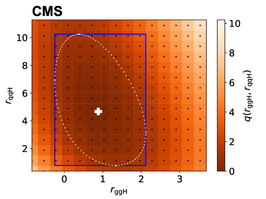
Figure 6: Values of $q(r_{\Pg\Pg\PH},r_{\PQq\PQq\PH})$ for Datacard 5 in a model with two parameters of interest $r_{\Pg\Pg\PH}$ and $r_{\PQq\PQq\PH}$. The orange scale shows the values obtained in Combine at the set of points indicated by the black dots, using the grid algorithm. The blue box is constructed using the cross algorithm with $(1-\alpha)=0.68$. The white cross and white dots indicate, respectively, the maximum likelihood estimates for $r_{\Pg\Pg\PH}$ and $r_{\PQq\PQq\PH}$ from the best fit, and the 68% confidence region obtained using the contour2d algorithm defined as the values of $(r_{\Pg\Pg\PH},r_{\PQq\PQq\PH})$ for which $q(r_{\Pg\Pg\PH},r_{\PQq\PQq\PH})=2.3$.

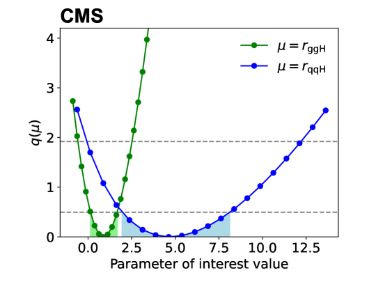
Figure 7: Example of $q(r_{\Pg\Pg\PH},\hat{r}_{\PQq\PQq\PH})$ and $q(r_{\PQq\PQq\PH},\hat{r}_{\Pg\Pg\PH})$ obtained from Combine with Datacard 5. The points indicate the values at which the functions are evaluated using the grid algorithm, and the shaded region indicates the 68% intervals on each parameter obtained using the singles algorithm. The horizontal dashed lines indicate the values of $q(\mu)$ used to define 68% and 95% intervals.

0.6.8 Goodness of fit tests and diagnostics

The GoodnessOfFit method can be used to perform a test of compatibility between the observed data and the statistical model. While the statistical model constructed by Combine is used as the null distribution, goodness of fit (GoF) tests do not have a well-defined alternative hypothesis, unlike conventional hypothesis tests.

The GoodnessOfFit method evaluates a test statistic for the observed data and generates the expected distribution of the test statistic under the null distribution using pseudo-data. In Combine this is done in two separate commands:

⬇

$ combine -M GoodnessOfFit <datacard.txt> --algo=<test-statistic>

$ combine -M GoodnessOfFit <datacard.txt> --algo=<test-statistic> --toys <N>

The first command evaluates the observed test statistic and the second determines the distribution of the test statistic under the null hypothesis using pseudo-data sets. The statistical model parameters used to specify the null hypothesis can be set using the --setParameters option.

All of the supported test statistics are based on binned data. For statistical models that include parametric shape analyses, an automatic binning is applied to the data to evaluate the probability density and calculate the test statistic, unless a specific binning is specified for the observables using the RooAbsReal::setBinning method. The following test statistics for the --algo option are supported in Combine:

• saturated: evaluates a GoF test statistic defined as

  $$t=-2\ln\frac{\mathcal{L}(\vec{\Phi})}{\mathcal{L}_{S}},$$ (37)

  where $i$ runs over all bins and $\mathcal{L}_{S}$ represents the likelihood for the saturated model [53].

• KS: evaluates the Kolmogorov–Smirnov test statistic [54, 55, 19], based on the largest difference between the cumulative distribution function and the empirical distribution function across all bins in all channels.

• AD: evaluates the Anderson–Darling test statistic based on the integral of the difference between the cumulative distribution function and the empirical distribution function across all bins in all channels. This test statistic gives more importance to the tails of the distribution in data [56, 57].

The output TTree contains a branch called limit that contains the value of the test statistic in each pseudo-data set if running with the option --toys, or from the observed data. These can be used to determine a $p$-value under the null hypothesis. Figure 8 shows the distribution of the saturated test statistic $t$ in pseudo-data sets using the statistical model constructed by Combine from Datacard 2 with default nuisance parameter values. The $p$-value is 0.73 and is computed from the distribution and the observed value of $t$. In this example, the template analysis in Datacard 2 was used to generate pseudo-data sets and calculate the corresponding $p$-value. The distribution of the test statistic has a peak close to the number of bins for the observable in the datacard, which is expected for this test statistic.

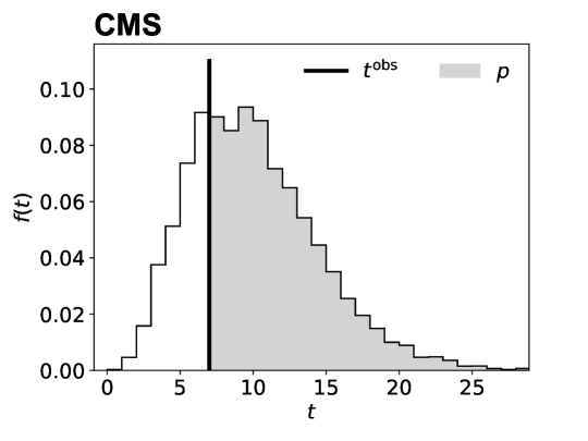
Figure 8: Distribution of the saturated test statistic $t$ in 10,000 pseudo-data sets using Datacard 2. The observed value of the test statistic is indicated by the black vertical line and the region used to determine $p$ is indicated by the light gray shaded region.

The method of pseudo-data generation can be modified using the options described in Section 0.6.3.

The ChannelCompatibilityCheck method is used to evaluate the compatibility between measurements of the signal rate in the $N_{c}$ separate channels defined in the statistical model. The method can be used with the default physics model and calculates the value of

$$q=-2\ln\left(\frac{\mathcal{L}(\hat{r})}{\mathcal{L}(\hat{r}_{1},\hat{r}_{2},...,\hat{r}_{N_{c}})}\right),$$ (38)

where each $r_{i}$ multiplies the rate of all signal processes in a specific channel $i$, and $\hat{r}$ denotes the maximum likelihood estimate.

The channel compatibility of the multi-signal Higgs boson analysis from Datacard 5 can be calculated using the command line below:

⬇

$ combine datacard-5-multi-signal.txt -M ChannelCompatibilityCheck --mass 125

The output from these commands is given below:

⬇

> --- ChannelCompatibilityCheck ---

> Nominal fit : r = 1.4812 -0.5987/+0.6644

> Alternate fit: r = 3.5554 -1.8576/+2.3619 in channel dijet

> Alternate fit: r = 1.1506 -0.6393/+0.6939 in channel incl

> Chi2-like compatibility variable: 1.5417

> Done in 0.00 min (cpu), 0.02 min (real)

These results are not expected to match those from the maximum likelihood estimates for the parameters $r_{\Pg\Pg\PH}$ and $r_{\PQq\PQq\PH}$ as the parameters in that model are related to the process signal multipliers instead of multipliers for the total signal in each channel. The compatibility variable in the output is the value of $q$. Assuming the values of $\hat{r_{i}}$ are normally distributed, this quantity can be converted to a $p$-value $p=\int_{q}^{\infty}\chi^{2}(x;N_{c}-1)\,\rd{x}$ where $\chi^{2}$ is a chi-squared distribution with $N_{c}-1$ degrees of freedom.

The output TTree contains the value of $q$ in the limit branch. If the option --saveFitResult is specified, the output ROOT file also contains two RooFitResult objects fit_nominal, and fit_alternate with the results of the two maximum likelihood optimizations used to calculate the numerator and denominator in $q$, respectively.

The FitDiagnostics method provides a number of diagnostic routines to investigate the statistical model. The method can be used with the default physics model and performs two optimizations of the parameters $\vec{\Phi}$ that maximize the function $\mathcal{L}(\vec{\Phi})$, the first with the parameter of interest $r$ allowed to vary and the second with $r$ set at a constant value of zero. The output TTree contains the maximum likelihood estimator for $r$ and an estimate of its uncertainty. In addition to the usual output file, an additional ROOT file is produced with the name fitDiagnostics$NAME.root. This file contains additional details about the optimizations performed that can be used to investigate the statistical model and the optimization procedure, the details of which are given in Table 0.6.8.

Additional output file contents from the FitDiagnostics method. Object Description nuisances_prefit RooArgSet containing the default values of $\vec{\nu}$, and their uncertainties estimated from their probability distributions. fit_b RooFitResult object containing the outcome of the maximum likelihood optimization with $r$ fixed to zero. fit_s RooFitResult object containing the outcome of the maximum likelihood optimization with $r$ allowed to vary. tree_prefit TTree of default values of $\vec{\nu}$ and $\vec{y}$. tree_fit_b TTree of maximum likelihood estimates $\hat{\hat{{\vec{\nu}}}}(0)$ and values of $\vec{y}$ from the maximum likelihood optimization fixing $r$ to zero. tree_fit_sb TTree of maximum likelihood estimates $\hat{\vec{\nu}}$ and values of $\vec{y}$ from the maximum likelihood optimization allowing $r$ to vary. Objects below are present only if the option --plots is included. covariance_fit_b TH2D covariance matrix of the parameters from the maximum likelihood optimization fixing $r$ to zero. covariance_fit_s TH2D covariance matrix of the parameters from the maximum likelihood optimization allowing $r$ to vary. channel_observable_prefit RooPlot plot of the probability density, normalized to the yield in data, projected onto each observable in each channel along with a histogram of the data. The statistical model parameters are set to their default values. channel_observable_fit_b Same as channel_observable_prefit, except the statistical model parameters are set to their maximum likelihood estimates from the optimization fixing $r$ to zero. channel_observable_fit_s Same as channel_observable_prefit, except the statistical model parameters are set to their maximum likelihood estimates from the optimization allowing $r$ to vary.

In addition to maximum likelihood estimates for all of the model parameters, these results contain estimates of their uncertainties. By default, the uncertainties for all nuisance parameters $\Delta\nu$ are estimated as $\Delta\nu_{k}=H^{-1}_{kk}$, where $H_{ij}$ is the Hessian matrix of $q(\hat{\vec{{\mu}}})$,

$$H_{ij}=\dfrac{\partial^{2}q}{\partial\nu_{i}\partial\nu_{j}}\bigg{\rvert}_{\vec{\Phi}=\hat{\vec{\Phi}}},$$ (39)

where $\hat{\vec{\Phi}}$ are the maximum likelihood estimates of the statistical model parameters. The accuracy can be improved by including the option --minos all, which determines the uncertainty for each nuisance parameter as,

$$\Delta^{\pm}\nu_{k}=\abs{\nu^{\pm}-\hat{\nu}},$$ (40)

where the range $\left(\nu^{-},\nu^{+}\right)$ is determined as the region for which $q(\nu)<1/2$, similar to the singles algorithm described in Section 0.6.7.

The results contained in this file can be used to study the additional constraints imposed by the observed data by considering the difference between the maximum likelihood estimates of the nuisance parameters (“post-fit”) and their uncertainties compared to their default (“pre-fit”) values.

The FitDiagnostics method can also be used to calculate nuisance parameter impacts [58] for statistical models with multiple parameters of interest, defined with respect to any particular parameter of interest $\mu$ for each nuisance parameter $\nu_{k}$ as,

$$\Delta\mu^{\pm}=\hat{\mu}\left(\hat{\nu}_{k}\pm\Delta^{\pm}\nu_{k}\right)-\hat{\mu},$$ (41)

where $\hat{\mu}(\nu_{k}\pm\Delta^{\pm}_{k})$ is the value of $\mu$ that maximizes the likelihood function when the nuisance parameter is shifted from its maximum likelihood estimator value by its uncertainty. Large impacts typically result from nuisance parameters that contribute significantly to the total uncertainty in $\mu$ and the sign of the impact indicates the sign of the (anti-)correlation between the parameter of interest and that nuisance parameter. These impacts provide diagnostic information that encapsulates both the constraints imposed on the nuisance parameter by the data and the correlation of that nuisance parameter with a particular parameter of interest. Figure 9 shows the impacts for the default physics model parameter $r$ calculated in the statistical analysis leading to the observation of four top quark production by the CMS Collaboration [22]. These impacts are calculated using both the observed data set (“obs.”) and an Asimov data set constructed assuming standard model production of four top quarks to obtain the expected (“exp.”) impacts.

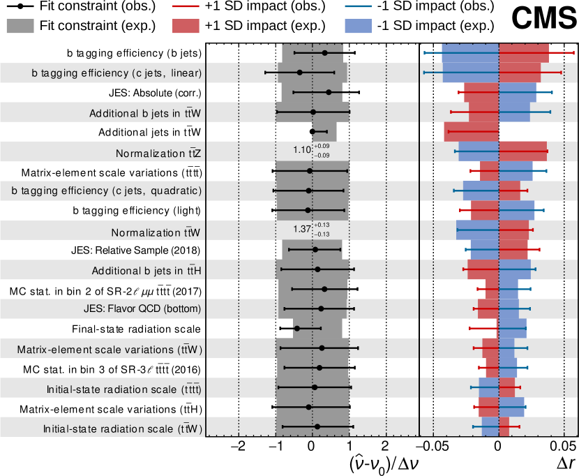
Figure 9: Example of nuisance parameter uncertainties and impacts calculated in Combine for the observation of four top quark production. Each row gives the name of the nuisance parameter, the difference in its maximum likelihood estimate $\hat{\nu}$ with respect to its default value $\nu_{0}$ relative to its uncertainty $\Delta\nu$, and the impact with respect to the default physics model parameter $\Delta r$. The nuisance parameter constraints and impacts are calculated using the observed data set (obs.) and an Asimov dataset constructed assuming standard model production of four top quarks (exp.). The red and blue lines in each row represent the positive impact $\Delta r^{+}$ and negative impact $\Delta r^{-}$, respectively, for the observed data. Similarly, the red and blue shaded boxes represent the same quantities for the Asimov dataset. The error bars on the fit constraint values indicate the ratio of $\Delta^{-}\nu$ or $\Delta^{+}\nu$, to their default values. The two numerical values displayed in the figure give the value of $\hat{\nu}^{+\Delta^{+}\nu}_{-\Delta^{-}\nu}$ for two rate parameters, which do not have well-defined default uncertainty values. Figure adapted from Ref. [22].

By including the option --saveShapes with this method, Combine saves additional ROOT TH1F histogram objects in the output file. These represent the contributions from each process in each channel of the statistical model evaluated at the default values of the parameters, and at the maximum likelihood estimates from the two optimizations. This allows a visualization of the pdfs of the primary observables at the pre-fit and post-fit values of the statistical model parameters individually for each process and each channel. For statistical models that include parametric shape analyses, an automatic binning is used to construct the histograms unless a particular binning is specified for the observables using the RooAbsReal::setBinning method. The total signal, total background, and total contributions in each channel are also saved as separate TH1F histogram objects. By adding the option --saveWithUncertainties, the output also includes estimates of the covariance between each of the bin yields, accounting for any correlations between the parameters of the statistical model. This is achieved using the RooFitResult::randomizePars() method from the results of the optimization. Figure 10 shows the distribution of the observable $x$ for the data and the background process in Datacard 2 using the default physics model. The uncertainties are estimated by sampling from the distributions $p(\nu|y)$ in the pre-fit case and from the covariance matrix of the model parameters obtained from a fit to the data shown assuming $r=0$ (post-fit). The change in the expected number of events in each bin $\lambda$ and their uncertainties $\Delta\lambda$ visually indicate the additional constraint imposed by the data on the statistical model parameters.

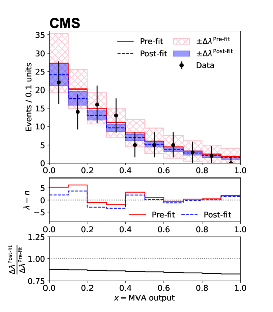
Figure 10: Distributions of the observable $x$ for the data and background process in Datacard 2 and their uncertainties. The upper panel shows the distribution for the default values of the nuisance parameters (red solid line, pre-fit) and for the maximum likelihood estimates assuming no signal (blue dashed line, post-fit). The pink hatched and blue shaded bands show the estimate of the uncertainty in each bin for the pre-fit and post-fit distributions, respectively. The middle panel shows the difference between the expected number of events in the background processes ($\lambda$) and the data ($n$) in the pre-fit (red solid line) and post-fit (blue dashed line) cases, and the lower panel shows the ratios of the estimated uncertainties of the post-fit distribution $\Delta\lambda^{\text{Post-fit}}$ to the pre-fit $\Delta\lambda^{\text{Pre-fit}}$ in each bin.

The FitDiagnostics method can be run with the --toys option such that the process normalization and bin yields in each channel resulting from each of the two optimizations performed using pseudo-data sets are stored, allowing for more detailed studies of the statistical model.

0.7 Summary

After a decade of development, the Combine package has become the main tool used for statistical analysis of data by the CMS Collaboration. The tool is based on the ROOT [1], RooFit [2], and RooStats [2] software packages to provide a command-line interface to several common statistical workflows used in high-energy physics. The statistical model is constructed from a text file provided by the user and a configurable physics model that encodes the parameters of interest and the nuisance parameters that model systematic uncertainties. The Combine package can perform a variety of statistical procedures including calculating confidence or credible intervals, evaluating profile likelihoods, and performing goodness of fit tests. The online documentation [12] contains comprehensive information on the capabilities and instructions for running the Combine package, as well as detailed instructions for its installation.

.8 The CMS Collaboration

Yerevan Physics Institute, Yerevan, Armenia A. Hayrapetyan, A. Tumasyan10009-0000-0684-6742

Institut für Hochenergiephysik, Vienna, Austria W. Adam0000-0001-9099-4341, J.W. Andrejkovic, T. Bergauer0000-0002-5786-0293, S. Chatterjee0000-0003-2660-0349, K. Damanakis0000-0001-5389-2872, M. Dragicevic0000-0003-1967-6783, P.S. Hussain0000-0002-4825-5278, M. Jeitler20000-0002-5141-9560, N. Krammer0000-0002-0548-0985, A. Li0000-0002-4547-116X, D. Liko0000-0002-3380-473X, I. Mikulec0000-0003-0385-2746, J. Schieck20000-0002-1058-8093, R. Schöfbeck0000-0002-2332-8784, D. Schwarz0000-0002-3821-7331, M. Sonawane0000-0003-0510-7010, S. Templ0000-0003-3137-5692, W. Waltenberger0000-0002-6215-7228, C.-E. Wulz20000-0001-9226-5812

Universiteit Antwerpen, Antwerpen, Belgium M.R. Darwish30000-0003-2894-2377, T. Janssen0000-0002-3998-4081, P. Van Mechelen0000-0002-8731-9051

Vrije Universiteit Brussel, Brussel, Belgium N. Breugelmans, J. D’Hondt0000-0002-9598-6241, S. Dansana0000-0002-7752-7471, A. De Moor0000-0001-5964-1935, M. Delcourt0000-0001-8206-1787, F. Heyen, S. Lowette0000-0003-3984-9987, I. Makarenko0000-0002-8553-4508, D. Müller0000-0002-1752-4527, S. Tavernier0000-0002-6792-9522, M. Tytgat40000-0002-3990-2074, G.P. Van Onsem0000-0002-1664-2337, S. Van Putte0000-0003-1559-3606, D. Vannerom0000-0002-2747-5095

Université Libre de Bruxelles, Bruxelles, Belgium B. Clerbaux0000-0001-8547-8211, A.K. Das, G. De Lentdecker0000-0001-5124-7693, H. Evard0009-0005-5039-1462, L. Favart0000-0003-1645-7454, P. Gianneios0009-0003-7233-0738, D. Hohov0000-0002-4760-1597, J. Jaramillo0000-0003-3885-6608, A. Khalilzadeh, F.A. Khan0009-0002-2039-277X, K. Lee0000-0003-0808-4184, M. Mahdavikhorrami0000-0002-8265-3595, A. Malara0000-0001-8645-9282, S. Paredes0000-0001-8487-9603, M.A. Shahzad, L. Thomas0000-0002-2756-3853, M. Vanden Bemden0009-0000-7725-7945, C. Vander Velde0000-0003-3392-7294, P. Vanlaer0000-0002-7931-4496

Ghent University, Ghent, Belgium M. De Coen0000-0002-5854-7442, D. Dobur0000-0003-0012-4866, G. Gokbulut0000-0002-0175-6454, Y. Hong0000-0003-4752-2458, J. Knolle0000-0002-4781-5704, L. Lambrecht0000-0001-9108-1560, D. Marckx0000-0001-6752-2290, G. Mestdach, K. Mota Amarilo0000-0003-1707-3348, A. Samalan, K. Skovpen0000-0002-1160-0621, N. Van Den Bossche0000-0003-2973-4991, J. van der Linden0000-0002-7174-781X, L. Wezenbeek0000-0001-6952-891X

Université Catholique de Louvain, Louvain-la-Neuve, Belgium A. Benecke0000-0003-0252-3609, A. Bethani0000-0002-8150-7043, G. Bruno0000-0001-8857-8197, C. Caputo0000-0001-7522-4808, J. De Favereau De Jeneret0000-0003-1775-8574, C. Delaere0000-0001-8707-6021, I.S. Donertas0000-0001-7485-412X, A. Giammanco0000-0001-9640-8294, A.O. Guzel0000-0002-9404-5933, Sa. Jain0000-0001-5078-3689, V. Lemaitre, J. Lidrych0000-0003-1439-0196, P. Mastrapasqua0000-0002-2043-2367, T.T. Tran0000-0003-3060-350X, S. Wertz0000-0002-8645-3670

Centro Brasileiro de Pesquisas Fisicas, Rio de Janeiro, Brazil G.A. Alves0000-0002-8369-1446, M. Alves Gallo Pereira0000-0003-4296-7028, E. Coelho0000-0001-6114-9907, G. Correia Silva0000-0001-6232-3591, C. Hensel0000-0001-8874-7624, T. Menezes De Oliveira0009-0009-4729-8354, A. Moraes0000-0002-5157-5686, P. Rebello Teles0000-0001-9029-8506, M. Soeiro, A. Vilela Pereira50000-0003-3177-4626

Universidade do Estado do Rio de Janeiro, Rio de Janeiro, Brazil W.L. Aldá Júnior0000-0001-5855-9817, M. Barroso Ferreira Filho0000-0003-3904-0571, H. Brandao Malbouisson0000-0002-1326-318X, W. Carvalho0000-0003-0738-6615, J. Chinellato6, E.M. Da Costa0000-0002-5016-6434, G.G. Da Silveira70000-0003-3514-7056, D. De Jesus Damiao0000-0002-3769-1680, S. Fonseca De Souza0000-0001-7830-0837, R. Gomes De Souza, M. Macedo0000-0002-6173-9859, J. Martins80000-0002-2120-2782, C. Mora Herrera0000-0003-3915-3170, L. Mundim0000-0001-9964-7805, H. Nogima0000-0001-7705-1066, J.P. Pinheiro0000-0002-3233-8247, A. Santoro0000-0002-0568-665X, A. Sznajder0000-0001-6998-1108, M. Thiel0000-0001-7139-7963

Universidade Estadual Paulista, Universidade Federal do ABC, São Paulo, Brazil C.A. Bernardes70000-0001-5790-9563, L. Calligaris0000-0002-9951-9448, T.R. Fernandez Perez Tomei0000-0002-1809-5226, E.M. Gregores0000-0003-0205-1672, I. Maietto Silverio0000-0003-3852-0266, P.G. Mercadante0000-0001-8333-4302, S.F. Novaes0000-0003-0471-8549, B. Orzari0000-0003-4232-4743, Sandra S. Padula0000-0003-3071-0559

Institute for Nuclear Research and Nuclear Energy, Bulgarian Academy of Sciences, Sofia, Bulgaria A. Aleksandrov0000-0001-6934-2541, G. Antchev0000-0003-3210-5037, R. Hadjiiska0000-0003-1824-1737, P. Iaydjiev0000-0001-6330-0607, M. Misheva0000-0003-4854-5301, M. Shopova0000-0001-6664-2493, G. Sultanov0000-0002-8030-3866

University of Sofia, Sofia, Bulgaria A. Dimitrov0000-0003-2899-701X, L. Litov0000-0002-8511-6883, B. Pavlov0000-0003-3635-0646, P. Petkov0000-0002-0420-9480, A. Petrov0009-0003-8899-1514, E. Shumka0000-0002-0104-2574

Instituto De Alta Investigación, Universidad de Tarapacá, Casilla 7 D, Arica, Chile S. Keshri0000-0003-3280-2350, S. Thakur0000-0002-1647-0360

Beihang University, Beijing, China T. Cheng0000-0003-2954-9315, T. Javaid0009-0007-2757-4054, L. Yuan0000-0002-6719-5397

Department of Physics, Tsinghua University, Beijing, China Z. Hu0000-0001-8209-4343, Z. Liang, J. Liu, K. Yi9^,100000-0002-2459-1824

Institute of High Energy Physics, Beijing, China G.M. Chen110000-0002-2629-5420, H.S. Chen110000-0001-8672-8227, M. Chen110000-0003-0489-9669, F. Iemmi0000-0001-5911-4051, C.H. Jiang, A. Kapoor120000-0002-1844-1504, H. Liao0000-0002-0124-6999, Z.-A. Liu130000-0002-2896-1386, R. Sharma140000-0003-1181-1426, J.N. Song13, J. Tao0000-0003-2006-3490, C. Wang11, J. Wang0000-0002-3103-1083, Z. Wang11, H. Zhang0000-0001-8843-5209, J. Zhao0000-0001-8365-7726

State Key Laboratory of Nuclear Physics and Technology, Peking University, Beijing, China A. Agapitos0000-0002-8953-1232, Y. Ban0000-0002-1912-0374, S. Deng0000-0002-2999-1843, B. Guo, C. Jiang0009-0008-6986-388X, A. Levin0000-0001-9565-4186, C. Li0000-0002-6339-8154, Q. Li0000-0002-8290-0517, Y. Mao, S. Qian, S.J. Qian0000-0002-0630-481X, X. Qin, X. Sun0000-0003-4409-4574, D. Wang0000-0002-9013-1199, H. Yang, L. Zhang0000-0001-7947-9007, Y. Zhao, C. Zhou0000-0001-5904-7258

Guangdong Provincial Key Laboratory of Nuclear Science and Guangdong-Hong Kong Joint Laboratory of Quantum Matter, South China Normal University, Guangzhou, China S. Yang0000-0002-2075-8631

Sun Yat-Sen University, Guangzhou, China Z. You0000-0001-8324-3291

University of Science and Technology of China, Hefei, China K. Jaffel0000-0001-7419-4248, N. Lu0000-0002-2631-6770

Nanjing Normal University, Nanjing, China G. Bauer15, B. Li, J. Zhang0000-0003-3314-2534

Institute of Modern Physics and Key Laboratory of Nuclear Physics and Ion-beam Application (MOE) - Fudan University, Shanghai, China X. Gao160000-0001-7205-2318

Zhejiang University, Hangzhou, Zhejiang, China Z. Lin0000-0003-1812-3474, C. Lu0000-0002-7421-0313, M. Xiao0000-0001-9628-9336

Universidad de Los Andes, Bogota, Colombia C. Avila0000-0002-5610-2693, D.A. Barbosa Trujillo, A. Cabrera0000-0002-0486-6296, C. Florez0000-0002-3222-0249, J. Fraga0000-0002-5137-8543, J.A. Reyes Vega

Universidad de Antioquia, Medellin, Colombia F. Ramirez0000-0002-7178-0484, C. Rendón, M. Rodriguez0000-0002-9480-213X, A.A. Ruales Barbosa0000-0003-0826-0803, J.D. Ruiz Alvarez0000-0002-3306-0363

University of Split, Faculty of Electrical Engineering, Mechanical Engineering and Naval Architecture, Split, Croatia D. Giljanovic0009-0005-6792-6881, N. Godinovic0000-0002-4674-9450, D. Lelas0000-0002-8269-5760, A. Sculac0000-0001-7938-7559

University of Split, Faculty of Science, Split, Croatia M. Kovac0000-0002-2391-4599, A. Petkovic, T. Sculac0000-0002-9578-4105

Institute Rudjer Boskovic, Zagreb, Croatia P. Bargassa0000-0001-8612-3332, V. Brigljevic0000-0001-5847-0062, B.K. Chitroda0000-0002-0220-8441, D. Ferencek0000-0001-9116-1202, K. Jakovcic, S. Mishra0000-0002-3510-4833, A. Starodumov170000-0001-9570-9255, T. Susa0000-0001-7430-2552

University of Cyprus, Nicosia, Cyprus A. Attikis0000-0002-4443-3794, K. Christoforou0000-0003-2205-1100, A. Hadjiagapiou, C. Leonidou, J. Mousa0000-0002-2978-2718, C. Nicolaou, L. Paizanos, F. Ptochos0000-0002-3432-3452, P.A. Razis0000-0002-4855-0162, H. Rykaczewski, H. Saka0000-0001-7616-2573, A. Stepennov0000-0001-7747-6582

Charles University, Prague, Czech Republic M. Finger0000-0002-7828-9970, M. Finger Jr.0000-0003-3155-2484, A. Kveton0000-0001-8197-1914

Universidad San Francisco de Quito, Quito, Ecuador E. Carrera Jarrin0000-0002-0857-8507

Academy of Scientific Research and Technology of the Arab Republic of Egypt, Egyptian Network of High Energy Physics, Cairo, Egypt Y. Assran18^,19, B. El-mahdy, S. Elgammal19

Center for High Energy Physics (CHEP-FU), Fayoum University, El-Fayoum, Egypt M.A. Mahmoud0000-0001-8692-5458, Y. Mohammed0000-0001-8399-3017

National Institute of Chemical Physics and Biophysics, Tallinn, Estonia K. Ehataht0000-0002-2387-4777, M. Kadastik, T. Lange0000-0001-6242-7331, S. Nandan0000-0002-9380-8919, C. Nielsen0000-0002-3532-8132, J. Pata0000-0002-5191-5759, M. Raidal0000-0001-7040-9491, L. Tani0000-0002-6552-7255, C. Veelken0000-0002-3364-916X

Department of Physics, University of Helsinki, Helsinki, Finland H. Kirschenmann0000-0001-7369-2536, K. Osterberg0000-0003-4807-0414, M. Voutilainen0000-0002-5200-6477

Helsinki Institute of Physics, Helsinki, Finland S. Bharthuar0000-0001-5871-9622, N. Bin Norjoharuddeen0000-0002-8818-7476, E. Brücken0000-0001-6066-8756, F. Garcia0000-0002-4023-7964, P. Inkaew0000-0003-4491-8983, K.T.S. Kallonen0000-0001-9769-7163, T. Lampén0000-0002-8398-4249, K. Lassila-Perini0000-0002-5502-1795, S. Lehti0000-0003-1370-5598, T. Lindén0009-0002-4847-8882, L. Martikainen0000-0003-1609-3515, M. Myllymäki0000-0003-0510-3810, M.m. Rantanen0000-0002-6764-0016, H. Siikonen0000-0003-2039-5874, J. Tuominiemi0000-0003-0386-8633

Lappeenranta-Lahti University of Technology, Lappeenranta, Finland P. Luukka0000-0003-2340-4641, H. Petrow0000-0002-1133-5485

IRFU, CEA, Université Paris-Saclay, Gif-sur-Yvette, France M. Besancon0000-0003-3278-3671, F. Couderc0000-0003-2040-4099, M. Dejardin0009-0008-2784-615X, D. Denegri, J.L. Faure, F. Ferri0000-0002-9860-101X, S. Ganjour0000-0003-3090-9744, P. Gras0000-0002-3932-5967, G. Hamel de Monchenault0000-0002-3872-3592, V. Lohezic0009-0008-7976-851X, J. Malcles0000-0002-5388-5565, F. Orlandi0009-0001-0547-7516, L. Portales0000-0002-9860-9185, A. Rosowsky0000-0001-7803-6650, M.Ö. Sahin0000-0001-6402-4050, A. Savoy-Navarro200000-0002-9481-5168, P. Simkina0000-0002-9813-372X, M. Titov0000-0002-1119-6614, M. Tornago0000-0001-6768-1056

Laboratoire Leprince-Ringuet, CNRS/IN2P3, Ecole Polytechnique, Institut Polytechnique de Paris, Palaiseau, France F. Beaudette0000-0002-1194-8556, P. Busson0000-0001-6027-4511, A. Cappati0000-0003-4386-0564, C. Charlot0000-0002-4087-8155, M. Chiusi0000-0002-1097-7304, F. Damas0000-0001-6793-4359, O. Davignon0000-0001-8710-992X, A. De Wit0000-0002-5291-1661, I.T. Ehle0000-0003-3350-5606, B.A. Fontana Santos Alves0000-0001-9752-0624, S. Ghosh0009-0006-5692-5688, A. Gilbert0000-0001-7560-5790, R. Granier de Cassagnac0000-0002-1275-7292, A. Hakimi0009-0008-2093-8131, B. Harikrishnan0000-0003-0174-4020, L. Kalipoliti0000-0002-5705-5059, G. Liu0000-0001-7002-0937, M. Nguyen0000-0001-7305-7102, C. Ochando0000-0002-3836-1173, R. Salerno0000-0003-3735-2707, J.B. Sauvan0000-0001-5187-3571, Y. Sirois0000-0001-5381-4807, L. Urda Gómez0000-0002-7865-5010, E. Vernazza0000-0003-4957-2782, A. Zabi0000-0002-7214-0673, A. Zghiche0000-0002-1178-1450

Université de Strasbourg, CNRS, IPHC UMR 7178, Strasbourg, France J.-L. Agram210000-0001-7476-0158, J. Andrea0000-0002-8298-7560, D. Apparu0009-0004-1837-0496, D. Bloch0000-0002-4535-5273, J.-M. Brom0000-0003-0249-3622, E.C. Chabert0000-0003-2797-7690, C. Collard0000-0002-5230-8387, S. Falke0000-0002-0264-1632, U. Goerlach0000-0001-8955-1666, R. Haeberle0009-0007-5007-6723, A.-C. Le Bihan0000-0002-8545-0187, M. Meena0000-0003-4536-3967, O. Poncet0000-0002-5346-2968, G. Saha0000-0002-6125-1941, M.A. Sessini0000-0003-2097-7065, P. Van Hove0000-0002-2431-3381, P. Vaucelle0000-0001-6392-7928

Centre de Calcul de l’Institut National de Physique Nucleaire et de Physique des Particules, CNRS/IN2P3, Villeurbanne, France A. Di Florio0000-0003-3719-8041

Institut de Physique des 2 Infinis de Lyon (IP2I ), Villeurbanne, France D. Amram, S. Beauceron0000-0002-8036-9267, B. Blancon0000-0001-9022-1509, G. Boudoul0009-0002-9897-8439, N. Chanon0000-0002-2939-5646, D. Contardo0000-0001-6768-7466, P. Depasse0000-0001-7556-2743, C. Dozen220000-0002-4301-634X, H. El Mamouni, J. Fay0000-0001-5790-1780, S. Gascon0000-0002-7204-1624, M. Gouzevitch0000-0002-5524-880X, C. Greenberg, G. Grenier0000-0002-1976-5877, B. Ille0000-0002-8679-3878, E. Jourd‘huy, I.B. Laktineh, M. Lethuillier0000-0001-6185-2045, L. Mirabito, S. Perries, A. Purohit0000-0003-0881-612X, M. Vander Donckt0000-0002-9253-8611, P. Verdier0000-0003-3090-2948, J. Xiao0000-0002-7860-3958

Georgian Technical University, Tbilisi, Georgia I. Lomidze0009-0002-3901-2765, T. Toriashvili230000-0003-1655-6874, Z. Tsamalaidze170000-0001-5377-3558

RWTH Aachen University, I. Physikalisches Institut, Aachen, Germany V. Botta0000-0003-1661-9513, L. Feld0000-0001-9813-8646, K. Klein0000-0002-1546-7880, M. Lipinski0000-0002-6839-0063, D. Meuser0000-0002-2722-7526, A. Pauls0000-0002-8117-5376, D. Pérez Adán0000-0003-3416-0726, N. Röwert0000-0002-4745-5470, M. Teroerde0000-0002-5892-1377

RWTH Aachen University, III. Physikalisches Institut A, Aachen, Germany S. Diekmann0009-0004-8867-0881, A. Dodonova0000-0002-5115-8487, N. Eich0000-0001-9494-4317, D. Eliseev0000-0001-5844-8156, F. Engelke0000-0002-9288-8144, J. Erdmann0000-0002-8073-2740, M. Erdmann0000-0002-1653-1303, P. Fackeldey0000-0003-4932-7162, B. Fischer0000-0002-3900-3482, T. Hebbeker0000-0002-9736-266X, K. Hoepfner0000-0002-2008-8148, F. Ivone0000-0002-2388-5548, A. Jung0000-0002-2511-1490, M.y. Lee0000-0002-4430-1695, F. Mausolf0000-0003-2479-8419, M. Merschmeyer0000-0003-2081-7141, A. Meyer0000-0001-9598-6623, S. Mukherjee0000-0001-6341-9982, D. Noll0000-0002-0176-2360, F. Nowotny, A. Pozdnyakov0000-0003-3478-9081, Y. Rath, W. Redjeb0000-0001-9794-8292, F. Rehm, H. Reithler0000-0003-4409-702X, V. Sarkisovi0000-0001-9430-5419, A. Schmidt0000-0003-2711-8984, A. Sharma0000-0002-5295-1460, J.L. Spah0000-0002-5215-3258, A. Stein0000-0003-0713-811X, F. Torres Da Silva De Araujo240000-0002-4785-3057, S. Wiedenbeck0000-0002-4692-9304, S. Zaleski

RWTH Aachen University, III. Physikalisches Institut B, Aachen, Germany C. Dziwok0000-0001-9806-0244, G. Flügge0000-0003-3681-9272, T. Kress0000-0002-2702-8201, A. Nowack0000-0002-3522-5926, O. Pooth0000-0001-6445-6160, A. Stahl0000-0002-8369-7506, T. Ziemons0000-0003-1697-2130, A. Zotz0000-0002-1320-1712

Deutsches Elektronen-Synchrotron, Hamburg, Germany H. Aarup Petersen0009-0005-6482-7466, M. Aldaya Martin0000-0003-1533-0945, J. Alimena0000-0001-6030-3191, S. Amoroso, Y. An0000-0003-1299-1879, J. Bach0000-0001-9572-6645, S. Baxter0009-0008-4191-6716, M. Bayatmakou0009-0002-9905-0667, H. Becerril Gonzalez0000-0001-5387-712X, O. Behnke0000-0002-4238-0991, A. Belvedere0000-0002-2802-8203, S. Bhattacharya0000-0002-3197-0048, F. Blekman250000-0002-7366-7098, K. Borras260000-0003-1111-249X, A. Campbell0000-0003-4439-5748, A. Cardini0000-0003-1803-0999, C. Cheng, F. Colombina0009-0008-7130-100X, S. Consuegra Rodríguez0000-0002-1383-1837, M. De Silva0000-0002-5804-6226, G. Eckerlin, D. Eckstein0000-0002-7366-6562, L.I. Estevez Banos0000-0001-6195-3102, O. Filatov0000-0001-9850-6170, E. Gallo250000-0001-7200-5175, A. Geiser0000-0003-0355-102X, V. Guglielmi0000-0003-3240-7393, M. Guthoff0000-0002-3974-589X, A. Hinzmann0000-0002-2633-4696, L. Jeppe0000-0002-1029-0318, B. Kaech0000-0002-1194-2306, M. Kasemann0000-0002-0429-2448, C. Kleinwort0000-0002-9017-9504, R. Kogler0000-0002-5336-4399, M. Komm0000-0002-7669-4294, D. Krücker0000-0003-1610-8844, W. Lange, D. Leyva Pernia0009-0009-8755-3698, K. Lipka270000-0002-8427-3748, W. Lohmann280000-0002-8705-0857, F. Lorkowski0000-0003-2677-3805, R. Mankel0000-0003-2375-1563, I.-A. Melzer-Pellmann0000-0001-7707-919X, M. Mendizabal Morentin0000-0002-6506-5177, A.B. Meyer0000-0001-8532-2356, G. Milella0000-0002-2047-951X, K. Moral Figueroa0000-0003-1987-1554, A. Mussgiller0000-0002-8331-8166, L.P. Nair0000-0002-2351-9265, J. Niedziela0000-0002-9514-0799, A. Nürnberg0000-0002-7876-3134, Y. Otarid, J. Park0000-0002-4683-6669, E. Ranken0000-0001-7472-5029, A. Raspereza0000-0003-2167-498X, D. Rastorguev0000-0001-6409-7794, J. Rübenach, L. Rygaard, A. Saggio0000-0002-7385-3317, M. Scham29^,260000-0001-9494-2151, S. Schnake260000-0003-3409-6584, P. Schütze0000-0003-4802-6990, C. Schwanenberger250000-0001-6699-6662, D. Selivanova0000-0002-7031-9434, K. Sharko0000-0002-7614-5236, M. Shchedrolosiev0000-0003-3510-2093, D. Stafford, F. Vazzoler0000-0001-8111-9318, A. Ventura Barroso0000-0003-3233-6636, R. Walsh0000-0002-3872-4114, D. Wang0000-0002-0050-612X, Q. Wang0000-0003-1014-8677, Y. Wen0000-0002-8724-9604, K. Wichmann, L. Wiens260000-0002-4423-4461, C. Wissing0000-0002-5090-8004, Y. Yang0009-0009-3430-0558, A. Zimermmane Castro Santos0000-0001-9302-3102

University of Hamburg, Hamburg, Germany A. Albrecht0000-0001-6004-6180, S. Albrecht0000-0002-5960-6803, M. Antonello0000-0001-9094-482X, S. Bein0000-0001-9387-7407, L. Benato0000-0001-5135-7489, S. Bollweg, M. Bonanomi0000-0003-3629-6264, P. Connor0000-0003-2500-1061, K. El Morabit0000-0001-5886-220X, Y. Fischer0000-0002-3184-1457, E. Garutti0000-0003-0634-5539, A. Grohsjean0000-0003-0748-8494, J. Haller0000-0001-9347-7657, H.R. Jabusch0000-0003-2444-1014, G. Kasieczka0000-0003-3457-2755, P. Keicher, R. Klanner0000-0002-7004-9227, W. Korcari0000-0001-8017-5502, T. Kramer0000-0002-7004-0214, C.c. Kuo, V. Kutzner0000-0003-1985-3807, F. Labe0000-0002-1870-9443, J. Lange0000-0001-7513-6330, A. Lobanov0000-0002-5376-0877, C. Matthies0000-0001-7379-4540, L. Moureaux0000-0002-2310-9266, M. Mrowietz, A. Nigamova0000-0002-8522-8500, Y. Nissan, A. Paasch0000-0002-2208-5178, K.J. Pena Rodriguez0000-0002-2877-9744, T. Quadfasel0000-0003-2360-351X, B. Raciti0009-0005-5995-6685, M. Rieger0000-0003-0797-2606, D. Savoiu0000-0001-6794-7475, J. Schindler0009-0006-6551-0660, P. Schleper0000-0001-5628-6827, M. Schröder0000-0001-8058-9828, J. Schwandt0000-0002-0052-597X, M. Sommerhalder0000-0001-5746-7371, H. Stadie0000-0002-0513-8119, G. Steinbrück0000-0002-8355-2761, A. Tews, M. Wolf0000-0003-3002-2430

Karlsruher Institut fuer Technologie, Karlsruhe, Germany S. Brommer0000-0001-8988-2035, M. Burkart, E. Butz0000-0002-2403-5801, T. Chwalek0000-0002-8009-3723, A. Dierlamm0000-0001-7804-9902, A. Droll, N. Faltermann0000-0001-6506-3107, M. Giffels0000-0003-0193-3032, A. Gottmann0000-0001-6696-349X, F. Hartmann300000-0001-8989-8387, R. Hofsaess0009-0008-4575-5729, M. Horzela0000-0002-3190-7962, U. Husemann0000-0002-6198-8388, J. Kieseler0000-0003-1644-7678, M. Klute0000-0002-0869-5631, R. Koppenhöfer0000-0002-6256-5715, J.M. Lawhorn0000-0002-8597-9259, M. Link, A. Lintuluoto0000-0002-0726-1452, B. Maier0000-0001-5270-7540, S. Maier0000-0001-9828-9778, S. Mitra0000-0002-3060-2278, M. Mormile0000-0003-0456-7250, Th. Müller0000-0003-4337-0098, M. Neukum, M. Oh0000-0003-2618-9203, E. Pfeffer0009-0009-1748-974X, M. Presilla0000-0003-2808-7315, G. Quast0000-0002-4021-4260, K. Rabbertz0000-0001-7040-9846, B. Regnery0000-0003-1539-923X, N. Shadskiy0000-0001-9894-2095, I. Shvetsov0000-0002-7069-9019, H.J. Simonis0000-0002-7467-2980, L. Sowa, L. Stockmeier, K. Tauqeer, M. Toms0000-0002-7703-3973, N. Trevisani0000-0002-5223-9342, R.F. Von Cube0000-0002-6237-5209, M. Wassmer0000-0002-0408-2811, S. Wieland0000-0003-3887-5358, F. Wittig, R. Wolf0000-0001-9456-383X, X. Zuo0000-0002-0029-493X

Institute of Nuclear and Particle Physics (INPP), NCSR Demokritos, Aghia Paraskevi, Greece G. Anagnostou, G. Daskalakis0000-0001-6070-7698, A. Kyriakis, A. Papadopoulos30, A. Stakia0000-0001-6277-7171

National and Kapodistrian University of Athens, Athens, Greece P. Kontaxakis0000-0002-4860-5979, G. Melachroinos, Z. Painesis0000-0001-5061-7031, I. Papavergou0000-0002-7992-2686, I. Paraskevas0000-0002-2375-5401, N. Saoulidou0000-0001-6958-4196, K. Theofilatos0000-0001-8448-883X, E. Tziaferi0000-0003-4958-0408, K. Vellidis0000-0001-5680-8357, I. Zisopoulos0000-0001-5212-4353

National Technical University of Athens, Athens, Greece G. Bakas0000-0003-0287-1937, T. Chatzistavrou, G. Karapostoli0000-0002-4280-2541, K. Kousouris0000-0002-6360-0869, I. Papakrivopoulos0000-0002-8440-0487, E. Siamarkou, G. Tsipolitis, A. Zacharopoulou

University of Ioánnina, Ioánnina, Greece K. Adamidis, I. Bestintzanos, I. Evangelou0000-0002-5903-5481, C. Foudas, C. Kamtsikis, P. Katsoulis, P. Kokkas0009-0009-3752-6253, P.G. Kosmoglou Kioseoglou0000-0002-7440-4396, N. Manthos0000-0003-3247-8909, I. Papadopoulos0000-0002-9937-3063, J. Strologas0000-0002-2225-7160

HUN-REN Wigner Research Centre for Physics, Budapest, Hungary C. Hajdu0000-0002-7193-800X, D. Horvath31^,320000-0003-0091-477X, K. Márton, A.J. Rádl330000-0001-8810-0388, F. Sikler0000-0001-9608-3901, V. Veszpremi0000-0001-9783-0315

MTA-ELTE Lendület CMS Particle and Nuclear Physics Group, Eötvös Loránd University, Budapest, Hungary M. Csanád0000-0002-3154-6925, K. Farkas0000-0003-1740-6974, A. Fehérkuti340000-0002-5043-2958, M.M.A. Gadallah350000-0002-8305-6661, Á. Kadlecsik0000-0001-5559-0106, P. Major0000-0002-5476-0414, G. Pásztor0000-0003-0707-9762, G.I. Veres0000-0002-5440-4356

Faculty of Informatics, University of Debrecen, Debrecen, Hungary B. Ujvari0000-0003-0498-4265, G. Zilizi0000-0002-0480-0000

Institute of Nuclear Research ATOMKI, Debrecen, Hungary G. Bencze, S. Czellar, J. Molnar, Z. Szillasi

Karoly Robert Campus, MATE Institute of Technology, Gyongyos, Hungary T. Csorgo340000-0002-9110-9663, T. Novak0000-0001-6253-4356

Panjab University, Chandigarh, India J. Babbar0000-0002-4080-4156, S. Bansal0000-0003-1992-0336, S.B. Beri, V. Bhatnagar0000-0002-8392-9610, G. Chaudhary0000-0003-0168-3336, S. Chauhan0000-0001-6974-4129, N. Dhingra360000-0002-7200-6204, A. Kaur0000-0002-1640-9180, A. Kaur0000-0003-3609-4777, H. Kaur0000-0002-8659-7092, M. Kaur0000-0002-3440-2767, S. Kumar0000-0001-9212-9108, K. Sandeep0000-0002-3220-3668, T. Sheokand, J.B. Singh0000-0001-9029-2462, A. Singla0000-0003-2550-139X

University of Delhi, Delhi, India A. Ahmed0000-0002-4500-8853, A. Bhardwaj0000-0002-7544-3258, A. Chhetri0000-0001-7495-1923, B.C. Choudhary0000-0001-5029-1887, A. Kumar0000-0003-3407-4094, A. Kumar0000-0002-5180-6595, M. Naimuddin0000-0003-4542-386X, K. Ranjan0000-0002-5540-3750, M.K. Saini, S. Saumya0000-0001-7842-9518

Saha Institute of Nuclear Physics, HBNI, Kolkata, India S. Baradia0000-0001-9860-7262, S. Barman370000-0001-8891-1674, S. Bhattacharya0000-0002-8110-4957, S. Das Gupta, S. Dutta0000-0001-9650-8121, S. Dutta, S. Sarkar

Indian Institute of Technology Madras, Madras, India M.M. Ameen0000-0002-1909-9843, P.K. Behera0000-0002-1527-2266, S.C. Behera0000-0002-0798-2727, S. Chatterjee0000-0003-0185-9872, G. Dash0000-0002-7451-4763, P. Jana0000-0001-5310-5170, P. Kalbhor0000-0002-5892-3743, S. Kamble0000-0001-7515-3907, J.R. Komaragiri380000-0002-9344-6655, D. Kumar380000-0002-6636-5331, P.R. Pujahari0000-0002-0994-7212, N.R. Saha0000-0002-7954-7898, A. Sharma0000-0002-0688-923X, A.K. Sikdar0000-0002-5437-5217, R.K. Singh, P. Verma, S. Verma0000-0003-1163-6955, A. Vijay

Tata Institute of Fundamental Research-A, Mumbai, India S. Dugad, M. Kumar0000-0003-0312-057X, G.B. Mohanty0000-0001-6850-7666, B. Parida0000-0001-9367-8061, M. Shelake, P. Suryadevara

Tata Institute of Fundamental Research-B, Mumbai, India A. Bala0000-0003-2565-1718, S. Banerjee0000-0002-7953-4683, R.M. Chatterjee, M. Guchait0009-0004-0928-7922, Sh. Jain0000-0003-1770-5309, A. Jaiswal, S. Kumar0000-0002-2405-915X, G. Majumder0000-0002-3815-5222, K. Mazumdar0000-0003-3136-1653, S. Parolia0000-0002-9566-2490, A. Thachayath0000-0001-6545-0350

National Institute of Science Education and Research, An OCC of Homi Bhabha National Institute, Bhubaneswar, Odisha, India S. Bahinipati390000-0002-3744-5332, C. Kar0000-0002-6407-6974, D. Maity400000-0002-1989-6703, P. Mal0000-0002-0870-8420, T. Mishra0000-0002-2121-3932, V.K. Muraleedharan Nair Bindhu400000-0003-4671-815X, K. Naskar400000-0003-0638-4378, A. Nayak400000-0002-7716-4981, S. Nayak, K. Pal, P. Sadangi, S.K. Swain0000-0001-6871-3937, S. Varghese400009-0000-1318-8266, D. Vats400009-0007-8224-4664

Indian Institute of Science Education and Research (IISER), Pune, India S. Acharya410009-0001-2997-7523, A. Alpana0000-0003-3294-2345, S. Dube0000-0002-5145-3777, B. Gomber410000-0002-4446-0258, P. Hazarika0009-0006-1708-8119, B. Kansal0000-0002-6604-1011, A. Laha0000-0001-9440-7028, B. Sahu410000-0002-8073-5140, S. Sharma0000-0001-6886-0726, K.Y. Vaish0009-0002-6214-5160

Isfahan University of Technology, Isfahan, Iran H. Bakhshiansohi420000-0001-5741-3357, A. Jafari430000-0001-7327-1870, M. Zeinali440000-0001-8367-6257

Institute for Research in Fundamental Sciences (IPM), Tehran, Iran S. Bashiri, S. Chenarani450000-0002-1425-076X, S.M. Etesami0000-0001-6501-4137, Y. Hosseini0000-0001-8179-8963, M. Khakzad0000-0002-2212-5715, E. Khazaie460000-0001-9810-7743, M. Mohammadi Najafabadi0000-0001-6131-5987, S. Tizchang470000-0002-9034-598X

University College Dublin, Dublin, Ireland M. Felcini0000-0002-2051-9331, M. Grunewald0000-0002-5754-0388

INFN Sezione di Bari^a, Università di Bari^b, Politecnico di Bari^c, Bari, Italy M. Abbrescia^a,b0000-0001-8727-7544, A. Colaleo^a,b0000-0002-0711-6319, D. Creanza^a,c0000-0001-6153-3044, B. D’Anzi^a,b0000-0002-9361-3142, N. De Filippis^a,c0000-0002-0625-6811, M. De Palma^a,b0000-0001-8240-1913, L. Fiore^a0000-0002-9470-1320, G. Iaselli^a,c0000-0003-2546-5341, L. Longo^a0000-0002-2357-7043, M. Louka^a,b, G. Maggi^a,c0000-0001-5391-7689, M. Maggi^a0000-0002-8431-3922, I. Margjeka^a0000-0002-3198-3025, V. Mastrapasqua^a,b0000-0002-9082-5924, S. My^a,b0000-0002-9938-2680, S. Nuzzo^a,b0000-0003-1089-6317, A. Pellecchia^a,b0000-0003-3279-6114, A. Pompili^a,b0000-0003-1291-4005, G. Pugliese^a,c0000-0001-5460-2638, R. Radogna^a,b0000-0002-1094-5038, D. Ramos^a0000-0002-7165-1017, A. Ranieri^a0000-0001-7912-4062, L. Silvestris^a0000-0002-8985-4891, F.M. Simone^a,c0000-0002-1924-983X, Ü. Sözbilir^a0000-0001-6833-3758, A. Stamerra^a,b0000-0003-1434-1968, D. Troiano^a,b0000-0001-7236-2025, R. Venditti^a,b0000-0001-6925-8649, P. Verwilligen^a0000-0002-9285-8631, A. Zaza^a,b0000-0002-0969-7284

INFN Sezione di Bologna^a, Università di Bologna^b, Bologna, Italy G. Abbiendi^a0000-0003-4499-7562, C. Battilana^a,b0000-0002-3753-3068, D. Bonacorsi^a,b0000-0002-0835-9574, L. Borgonovi^a0000-0001-8679-4443, P. Capiluppi^a,b0000-0003-4485-1897, A. Castro${}^{\textrm{\textdagger}}$^a,b0000-0003-2527-0456, F.R. Cavallo^a0000-0002-0326-7515, M. Cuffiani^a,b0000-0003-2510-5039, G.M. Dallavalle^a0000-0002-8614-0420, T. Diotalevi^a,b0000-0003-0780-8785, F. Fabbri^a0000-0002-8446-9660, A. Fanfani^a,b0000-0003-2256-4117, D. Fasanella^a0000-0002-2926-2691, P. Giacomelli^a0000-0002-6368-7220, L. Giommi^a,b0000-0003-3539-4313, C. Grandi^a0000-0001-5998-3070, L. Guiducci^a,b0000-0002-6013-8293, S. Lo Meo^a,480000-0003-3249-9208, M. Lorusso^a,b0000-0003-4033-4956, L. Lunerti^a0000-0002-8932-0283, S. Marcellini^a0000-0002-1233-8100, G. Masetti^a0000-0002-6377-800X, F.L. Navarria^a,b0000-0001-7961-4889, G. Paggi^a,b0009-0005-7331-1488, A. Perrotta^a0000-0002-7996-7139, F. Primavera^a,b0000-0001-6253-8656, A.M. Rossi^a,b0000-0002-5973-1305, S. Rossi Tisbeni^a,b0000-0001-6776-285X, T. Rovelli^a,b0000-0002-9746-4842, G.P. Siroli^a,b0000-0002-3528-4125

INFN Sezione di Catania^a, Università di Catania^b, Catania, Italy S. Costa^a,b,490000-0001-9919-0569, A. Di Mattia^a0000-0002-9964-015X, A. Lapertosa^a0000-0001-6246-6787, R. Potenza^a,b, A. Tricomi^a,b,490000-0002-5071-5501, C. Tuve^a,b0000-0003-0739-3153

INFN Sezione di Firenze^a, Università di Firenze^b, Firenze, Italy P. Assiouras^a0000-0002-5152-9006, G. Barbagli^a0000-0002-1738-8676, G. Bardelli^a,b0000-0002-4662-3305, B. Camaiani^a,b0000-0002-6396-622X, A. Cassese^a0000-0003-3010-4516, R. Ceccarelli^a0000-0003-3232-9380, V. Ciulli^a,b0000-0003-1947-3396, C. Civinini^a0000-0002-4952-3799, R. D’Alessandro^a,b0000-0001-7997-0306, E. Focardi^a,b0000-0002-3763-5267, T. Kello^a, G. Latino^a,b0000-0002-4098-3502, P. Lenzi^a,b0000-0002-6927-8807, M. Lizzo^a0000-0001-7297-2624, M. Meschini^a0000-0002-9161-3990, S. Paoletti^a0000-0003-3592-9509, A. Papanastassiou^a,b, G. Sguazzoni^a0000-0002-0791-3350, L. Viliani^a0000-0002-1909-6343

INFN Laboratori Nazionali di Frascati, Frascati, Italy L. Benussi0000-0002-2363-8889, S. Bianco0000-0002-8300-4124, S. Meola500000-0002-8233-7277, D. Piccolo0000-0001-5404-543X

INFN Sezione di Genova^a, Università di Genova^b, Genova, Italy P. Chatagnon^a0000-0002-4705-9582, F. Ferro^a0000-0002-7663-0805, E. Robutti^a0000-0001-9038-4500, S. Tosi^a,b0000-0002-7275-9193

INFN Sezione di Milano-Bicocca^a, Università di Milano-Bicocca^b, Milano, Italy A. Benaglia^a0000-0003-1124-8450, G. Boldrini^a,b0000-0001-5490-605X, F. Brivio^a0000-0001-9523-6451, F. Cetorelli^a,b0000-0002-3061-1553, F. De Guio^a,b0000-0001-5927-8865, M.E. Dinardo^a,b0000-0002-8575-7250, P. Dini^a0000-0001-7375-4899, S. Gennai^a0000-0001-5269-8517, R. Gerosa^a,b0000-0001-8359-3734, A. Ghezzi^a,b0000-0002-8184-7953, P. Govoni^a,b0000-0002-0227-1301, L. Guzzi^a0000-0002-3086-8260, M.T. Lucchini^a,b0000-0002-7497-7450, M. Malberti^a0000-0001-6794-8419, S. Malvezzi^a0000-0002-0218-4910, A. Massironi^a0000-0002-0782-0883, D. Menasce^a0000-0002-9918-1686, L. Moroni^a0000-0002-8387-762X, M. Paganoni^a,b0000-0003-2461-275X, S. Palluotto^a,b0009-0009-1025-6337, D. Pedrini^a0000-0003-2414-4175, A. Perego^a,b0009-0002-5210-6213, B.S. Pinolini^a, G. Pizzati^a,b, S. Ragazzi^a,b0000-0001-8219-2074, T. Tabarelli de Fatis^a,b0000-0001-6262-4685

INFN Sezione di Napoli^a, Università di Napoli ’Federico II’^b, Napoli, Italy; Università della Basilicata^c, Potenza, Italy; Scuola Superiore Meridionale (SSM)^d, Napoli, Italy S. Buontempo^a0000-0001-9526-556X, A. Cagnotta^a,b0000-0002-8801-9894, F. Carnevali^a,b, N. Cavallo^a,c0000-0003-1327-9058, F. Fabozzi^a,c0000-0001-9821-4151, A.O.M. Iorio^a,b0000-0002-3798-1135, L. Lista^a,b,510000-0001-6471-5492, P. Paolucci^a,300000-0002-8773-4781, B. Rossi^a0000-0002-0807-8772

INFN Sezione di Padova^a, Università di Padova^b, Padova, Italy; Università di Trento^c, Trento, Italy R. Ardino^a0000-0001-8348-2962, P. Azzi^a0000-0002-3129-828X, N. Bacchetta^a,520000-0002-2205-5737, D. Bisello^a,b0000-0002-2359-8477, P. Bortignon^a0000-0002-5360-1454, G. Bortolato^a,b, A. Bragagnolo^a,b0000-0003-3474-2099, A.C.M. Bulla^a0000-0001-5924-4286, R. Carlin^a,b0000-0001-7915-1650, P. Checchia^a0000-0002-8312-1531, T. Dorigo^a0000-0002-1659-8727, U. Gasparini^a,b0000-0002-7253-2669, A. Gozzelino^a0000-0002-6284-1126, M. Gulmini^a,530000-0003-4198-4336, E. Lusiani^a0000-0001-8791-7978, M. Margoni^a,b0000-0003-1797-4330, A.T. Meneguzzo^a,b0000-0002-5861-8140, M. Migliorini^a,b0000-0002-5441-7755, J. Pazzini^a,b0000-0002-1118-6205, P. Ronchese^a,b0000-0001-7002-2051, R. Rossin^a,b0000-0003-3466-7500, F. Simonetto^a,b0000-0002-8279-2464, G. Strong^a0000-0002-4640-6108, M. Tosi^a,b0000-0003-4050-1769, A. Triossi^a,b0000-0001-5140-9154, M. Zanetti^a,b0000-0003-4281-4582, P. Zotto^a,b0000-0003-3953-5996, A. Zucchetta^a,b0000-0003-0380-1172, G. Zumerle^a,b0000-0003-3075-2679

INFN Sezione di Pavia^a, Università di Pavia^b, Pavia, Italy C. Aimè^a0000-0003-0449-4717, A. Braghieri^a0000-0002-9606-5604, S. Calzaferri^a0000-0002-1162-2505, D. Fiorina^a0000-0002-7104-257X, P. Montagna^a,b0000-0001-9647-9420, V. Re^a0000-0003-0697-3420, C. Riccardi^a,b0000-0003-0165-3962, P. Salvini^a0000-0001-9207-7256, I. Vai^a,b0000-0003-0037-5032, P. Vitulo^a,b0000-0001-9247-7778

INFN Sezione di Perugia^a, Università di Perugia^b, Perugia, Italy S. Ajmal^a,b0000-0002-2726-2858, M.E. Ascioti^a,b, G.M. Bilei^a0000-0002-4159-9123, C. Carrivale^a,b, D. Ciangottini^a,b0000-0002-0843-4108, L. Fanò^a,b0000-0002-9007-629X, M. Magherini^a,b0000-0003-4108-3925, V. Mariani^a,b0000-0001-7108-8116, M. Menichelli^a0000-0002-9004-735X, F. Moscatelli^a,540000-0002-7676-3106, A. Rossi^a,b0000-0002-2031-2955, A. Santocchia^a,b0000-0002-9770-2249, D. Spiga^a0000-0002-2991-6384, T. Tedeschi^a,b0000-0002-7125-2905

INFN Sezione di Pisa^a, Università di Pisa^b, Scuola Normale Superiore di Pisa^c, Pisa, Italy; Università di Siena^d, Siena, Italy C.A. Alexe^a,c0000-0003-4981-2790, P. Asenov^a,b0000-0003-2379-9903, P. Azzurri^a0000-0002-1717-5654, G. Bagliesi^a0000-0003-4298-1620, R. Bhattacharya^a0000-0002-7575-8639, L. Bianchini^a,b0000-0002-6598-6865, T. Boccali^a0000-0002-9930-9299, E. Bossini^a0000-0002-2303-2588, D. Bruschini^a,c0000-0001-7248-2967, R. Castaldi^a0000-0003-0146-845X, M.A. Ciocci^a,b0000-0003-0002-5462, M. Cipriani^a,b0000-0002-0151-4439, V. D’Amante^a,d0000-0002-7342-2592, R. Dell’Orso^a0000-0003-1414-9343, S. Donato^a0000-0001-7646-4977, A. Giassi^a0000-0001-9428-2296, F. Ligabue^a,c0000-0002-1549-7107, D. Matos Figueiredo^a0000-0003-2514-6930, A. Messineo^a,b0000-0001-7551-5613, M. Musich^a,b0000-0001-7938-5684, F. Palla^a0000-0002-6361-438X, A. Rizzi^a,b0000-0002-4543-2718, G. Rolandi^a,c0000-0002-0635-274X, S. Roy Chowdhury^a0000-0001-5742-5593, T. Sarkar^a0000-0003-0582-4167, A. Scribano^a0000-0002-4338-6332, P. Spagnolo^a0000-0001-7962-5203, R. Tenchini^a0000-0003-2574-4383, G. Tonelli^a,b0000-0003-2606-9156, N. Turini^a,d0000-0002-9395-5230, F. Vaselli^a,c0009-0008-8227-0755, A. Venturi^a0000-0002-0249-4142, P.G. Verdini^a0000-0002-0042-9507

INFN Sezione di Roma^a, Sapienza Università di Roma^b, Roma, Italy C. Baldenegro Barrera^a,b0000-0002-6033-8885, P. Barria^a0000-0002-3924-7380, C. Basile^a,b0000-0003-4486-6482, M. Campana^a,b0000-0001-5425-723X, F. Cavallari^a0000-0002-1061-3877, L. Cunqueiro Mendez^a,b0000-0001-6764-5370, D. Del Re^a,b0000-0003-0870-5796, E. Di Marco^a0000-0002-5920-2438, M. Diemoz^a0000-0002-3810-8530, F. Errico^a,b0000-0001-8199-370X, E. Longo^a,b0000-0001-6238-6787, J. Mijuskovic^a,b0009-0009-1589-9980, G. Organtini^a,b0000-0002-3229-0781, F. Pandolfi^a0000-0001-8713-3874, R. Paramatti^a,b0000-0002-0080-9550, C. Quaranta^a,b0000-0002-0042-6891, S. Rahatlou^a,b0000-0001-9794-3360, C. Rovelli^a0000-0003-2173-7530, F. Santanastasio^a,b0000-0003-2505-8359, L. Soffi^a0000-0003-2532-9876

INFN Sezione di Torino^a, Università di Torino^b, Torino, Italy; Università del Piemonte Orientale^c, Novara, Italy N. Amapane^a,b0000-0001-9449-2509, R. Arcidiacono^a,c0000-0001-5904-142X, S. Argiro^a,b0000-0003-2150-3750, M. Arneodo^a,c0000-0002-7790-7132, N. Bartosik^a0000-0002-7196-2237, R. Bellan^a,b0000-0002-2539-2376, A. Bellora^a,b0000-0002-2753-5473, C. Biino^a0000-0002-1397-7246, C. Borca^a,b0009-0009-2769-5950, N. Cartiglia^a0000-0002-0548-9189, M. Costa^a,b0000-0003-0156-0790, R. Covarelli^a,b0000-0003-1216-5235, N. Demaria^a0000-0003-0743-9465, L. Finco^a0000-0002-2630-5465, M. Grippo^a,b0000-0003-0770-269X, B. Kiani^a,b0000-0002-1202-7652, F. Legger^a0000-0003-1400-0709, F. Luongo^a,b0000-0003-2743-4119, C. Mariotti^a0000-0002-6864-3294, L. Markovic^a,b0000-0001-7746-9868, S. Maselli^a0000-0001-9871-7859, A. Mecca^a,b0000-0003-2209-2527, L. Menzio^a,b, P. Meridiani^a0000-0002-8480-2259, E. Migliore^a,b0000-0002-2271-5192, M. Monteno^a0000-0002-3521-6333, R. Mulargia^a0000-0003-2437-013X, M.M. Obertino^a,b0000-0002-8781-8192, G. Ortona^a0000-0001-8411-2971, L. Pacher^a,b0000-0003-1288-4838, N. Pastrone^a0000-0001-7291-1979, M. Pelliccioni^a0000-0003-4728-6678, M. Ruspa^a,c0000-0002-7655-3475, F. Siviero^a,b0000-0002-4427-4076, V. Sola^a,b0000-0001-6288-951X, A. Solano^a,b0000-0002-2971-8214, A. Staiano^a0000-0003-1803-624X, C. Tarricone^a,b0000-0001-6233-0513, D. Trocino^a0000-0002-2830-5872, G. Umoret^a,b0000-0002-6674-7874, R. White^a,b0000-0001-5793-526X

INFN Sezione di Trieste^a, Università di Trieste^b, Trieste, Italy S. Belforte^a0000-0001-8443-4460, V. Candelise^a,b0000-0002-3641-5983, M. Casarsa^a0000-0002-1353-8964, F. Cossutti^a0000-0001-5672-214X, K. De Leo^a0000-0002-8908-409X, G. Della Ricca^a,b0000-0003-2831-6982

Kyungpook National University, Daegu, Korea S. Dogra0000-0002-0812-0758, J. Hong0000-0002-9463-4922, C. Huh0000-0002-8513-2824, B. Kim0000-0002-9539-6815, J. Kim, D. Lee, H. Lee, S.W. Lee0000-0002-1028-3468, C.S. Moon0000-0001-8229-7829, Y.D. Oh0000-0002-7219-9931, M.S. Ryu0000-0002-1855-180X, S. Sekmen0000-0003-1726-5681, B. Tae, Y.C. Yang0000-0003-1009-4621

Department of Mathematics and Physics - GWNU, Gangneung, Korea M.S. Kim0000-0003-0392-8691

Chonnam National University, Institute for Universe and Elementary Particles, Kwangju, Korea G. Bak0000-0002-0095-8185, P. Gwak0009-0009-7347-1480, H. Kim0000-0001-8019-9387, D.H. Moon0000-0002-5628-9187

Hanyang University, Seoul, Korea E. Asilar0000-0001-5680-599X, J. Choi0000-0002-6024-0992, D. Kim0000-0002-8336-9182, T.J. Kim0000-0001-8336-2434, J.A. Merlin, Y. Ryou

Korea University, Seoul, Korea S. Choi0000-0001-6225-9876, S. Han, B. Hong0000-0002-2259-9929, K. Lee, K.S. Lee0000-0002-3680-7039, S. Lee0000-0001-9257-9643, J. Yoo0000-0003-0463-3043

Kyung Hee University, Department of Physics, Seoul, Korea J. Goh0000-0002-1129-2083, S. Yang0000-0001-6905-6553

Sejong University, Seoul, Korea H. S. Kim0000-0002-6543-9191, Y. Kim, S. Lee

Seoul National University, Seoul, Korea J. Almond, J.H. Bhyun, J. Choi0000-0002-2483-5104, J. Choi, W. Jun0009-0001-5122-4552, J. Kim0000-0001-9876-6642, S. Ko0000-0003-4377-9969, H. Kwon0009-0002-5165-5018, H. Lee0000-0002-1138-3700, J. Lee0000-0001-6753-3731, J. Lee0000-0002-5351-7201, B.H. Oh0000-0002-9539-7789, S.B. Oh0000-0003-0710-4956, H. Seo0000-0002-3932-0605, U.K. Yang, I. Yoon0000-0002-3491-8026

University of Seoul, Seoul, Korea W. Jang0000-0002-1571-9072, D.Y. Kang, Y. Kang0000-0001-6079-3434, S. Kim0000-0002-8015-7379, B. Ko, J.S.H. Lee0000-0002-2153-1519, Y. Lee0000-0001-5572-5947, I.C. Park0000-0003-4510-6776, Y. Roh, I.J. Watson0000-0003-2141-3413

Yonsei University, Department of Physics, Seoul, Korea S. Ha0000-0003-2538-1551, H.D. Yoo0000-0002-3892-3500

Sungkyunkwan University, Suwon, Korea M. Choi0000-0002-4811-626X, M.R. Kim0000-0002-2289-2527, H. Lee, Y. Lee0000-0001-6954-9964, I. Yu0000-0003-1567-5548

College of Engineering and Technology, American University of the Middle East (AUM), Dasman, Kuwait T. Beyrouthy

Riga Technical University, Riga, Latvia K. Dreimanis0000-0003-0972-5641, A. Gaile0000-0003-1350-3523, G. Pikurs, A. Potrebko0000-0002-3776-8270, M. Seidel0000-0003-3550-6151, D. Sidiropoulos Kontos

University of Latvia (LU), Riga, Latvia N.R. Strautnieks0000-0003-4540-9048

Vilnius University, Vilnius, Lithuania M. Ambrozas0000-0003-2449-0158, A. Juodagalvis0000-0002-1501-3328, A. Rinkevicius0000-0002-7510-255X, G. Tamulaitis0000-0002-2913-9634

National Centre for Particle Physics, Universiti Malaya, Kuala Lumpur, Malaysia I. Yusuff550000-0003-2786-0732, Z. Zolkapli

Universidad de Sonora (UNISON), Hermosillo, Mexico J.F. Benitez0000-0002-2633-6712, A. Castaneda Hernandez0000-0003-4766-1546, H.A. Encinas Acosta, L.G. Gallegos Maríñez, M. León Coello0000-0002-3761-911X, J.A. Murillo Quijada0000-0003-4933-2092, A. Sehrawat0000-0002-6816-7814, L. Valencia Palomo0000-0002-8736-440X

Centro de Investigacion y de Estudios Avanzados del IPN, Mexico City, Mexico G. Ayala0000-0002-8294-8692, H. Castilla-Valdez0009-0005-9590-9958, H. Crotte Ledesma, E. De La Cruz-Burelo0000-0002-7469-6974, I. Heredia-De La Cruz560000-0002-8133-6467, R. Lopez-Fernandez0000-0002-2389-4831, J. Mejia Guisao0000-0002-1153-816X, C.A. Mondragon Herrera, A. Sánchez Hernández0000-0001-9548-0358

Universidad Iberoamericana, Mexico City, Mexico C. Oropeza Barrera0000-0001-9724-0016, D.L. Ramirez Guadarrama, M. Ramírez García0000-0002-4564-3822

Benemerita Universidad Autonoma de Puebla, Puebla, Mexico I. Bautista0000-0001-5873-3088, I. Pedraza0000-0002-2669-4659, H.A. Salazar Ibarguen0000-0003-4556-7302, C. Uribe Estrada0000-0002-2425-7340

University of Montenegro, Podgorica, Montenegro I. Bubanja0009-0005-4364-277X, N. Raicevic0000-0002-2386-2290

University of Canterbury, Christchurch, New Zealand P.H. Butler0000-0001-9878-2140

National Centre for Physics, Quaid-I-Azam University, Islamabad, Pakistan A. Ahmad0000-0002-4770-1897, M.I. Asghar, A. Awais0000-0003-3563-257X, M.I.M. Awan, H.R. Hoorani0000-0002-0088-5043, W.A. Khan0000-0003-0488-0941

AGH University of Krakow, Faculty of Computer Science, Electronics and Telecommunications, Krakow, Poland V. Avati, L. Grzanka0000-0002-3599-854X, M. Malawski0000-0001-6005-0243

National Centre for Nuclear Research, Swierk, Poland H. Bialkowska0000-0002-5956-6258, M. Bluj0000-0003-1229-1442, M. Górski0000-0003-2146-187X, M. Kazana0000-0002-7821-3036, M. Szleper0000-0002-1697-004X, P. Zalewski0000-0003-4429-2888

Institute of Experimental Physics, Faculty of Physics, University of Warsaw, Warsaw, Poland K. Bunkowski0000-0001-6371-9336, K. Doroba0000-0002-7818-2364, A. Kalinowski0000-0002-1280-5493, M. Konecki0000-0001-9482-4841, J. Krolikowski0000-0002-3055-0236, A. Muhammad0000-0002-7535-7149

Warsaw University of Technology, Warsaw, Poland K. Pozniak0000-0001-5426-1423, W. Zabolotny0000-0002-6833-4846

Laboratório de Instrumentação e Física Experimental de Partículas, Lisboa, Portugal M. Araujo0000-0002-8152-3756, D. Bastos0000-0002-7032-2481, C. Beirão Da Cruz E Silva0000-0002-1231-3819, A. Boletti0000-0003-3288-7737, M. Bozzo0000-0002-1715-0457, T. Camporesi0000-0001-5066-1876, G. Da Molin0000-0003-2163-5569, P. Faccioli0000-0003-1849-6692, M. Gallinaro0000-0003-1261-2277, J. Hollar0000-0002-8664-0134, N. Leonardo0000-0002-9746-4594, G.B. Marozzo, T. Niknejad0000-0003-3276-9482, A. Petrilli0000-0003-0887-1882, M. Pisano0000-0002-0264-7217, J. Seixas0000-0002-7531-0842, J. Varela0000-0003-2613-3146, J.W. Wulff

Faculty of Physics, University of Belgrade, Belgrade, Serbia P. Adzic0000-0002-5862-7397, P. Milenovic0000-0001-7132-3550

VINCA Institute of Nuclear Sciences, University of Belgrade, Belgrade, Serbia M. Dordevic0000-0002-8407-3236, J. Milosevic0000-0001-8486-4604, L. Nadderd0000-0003-4702-4598, V. Rekovic

Centro de Investigaciones Energéticas Medioambientales y Tecnológicas (CIEMAT), Madrid, Spain J. Alcaraz Maestre0000-0003-0914-7474, Cristina F. Bedoya0000-0001-8057-9152, Oliver M. Carretero0000-0002-6342-6215, M. Cepeda0000-0002-6076-4083, M. Cerrada0000-0003-0112-1691, N. Colino0000-0002-3656-0259, B. De La Cruz0000-0001-9057-5614, A. Delgado Peris0000-0002-8511-7958, A. Escalante Del Valle0000-0002-9702-6359, D. Fernández Del Val0000-0003-2346-1590, J.P. Fernández Ramos0000-0002-0122-313X, J. Flix0000-0003-2688-8047, M.C. Fouz0000-0003-2950-976X, O. Gonzalez Lopez0000-0002-4532-6464, S. Goy Lopez0000-0001-6508-5090, J.M. Hernandez0000-0001-6436-7547, M.I. Josa0000-0002-4985-6964, E. Martin Viscasillas0000-0001-8808-4533, D. Moran0000-0002-1941-9333, C. M. Morcillo Perez0000-0001-9634-848X, Á. Navarro Tobar0000-0003-3606-1780, C. Perez Dengra0000-0003-2821-4249, A. Pérez-Calero Yzquierdo0000-0003-3036-7965, J. Puerta Pelayo0000-0001-7390-1457, I. Redondo0000-0003-3737-4121, S. Sánchez Navas0000-0001-6129-9059, J. Sastre0000-0002-1654-2846, J. Vazquez Escobar0000-0002-7533-2283

Universidad Autónoma de Madrid, Madrid, Spain J.F. de Trocóniz0000-0002-0798-9806

Universidad de Oviedo, Instituto Universitario de Ciencias y Tecnologías Espaciales de Asturias (ICTEA), Oviedo, Spain B. Alvarez Gonzalez0000-0001-7767-4810, J. Cuevas0000-0001-5080-0821, J. Fernandez Menendez0000-0002-5213-3708, S. Folgueras0000-0001-7191-1125, I. Gonzalez Caballero0000-0002-8087-3199, J.R. González Fernández0000-0002-4825-8188, P. Leguina0000-0002-0315-4107, E. Palencia Cortezon0000-0001-8264-0287, C. Ramón Álvarez0000-0003-1175-0002, V. Rodríguez Bouza0000-0002-7225-7310, A. Soto Rodríguez0000-0002-2993-8663, A. Trapote0000-0002-4030-2551, C. Vico Villalba0000-0002-1905-1874, P. Vischia0000-0002-7088-8557

Instituto de Física de Cantabria (IFCA), CSIC-Universidad de Cantabria, Santander, Spain S. Bhowmik0000-0003-1260-973X, S. Blanco Fernández0000-0001-7301-0670, J.A. Brochero Cifuentes0000-0003-2093-7856, I.J. Cabrillo0000-0002-0367-4022, A. Calderon0000-0002-7205-2040, J. Duarte Campderros0000-0003-0687-5214, M. Fernandez0000-0002-4824-1087, G. Gomez0000-0002-1077-6553, C. Lasaosa García0000-0003-2726-7111, R. Lopez Ruiz0009-0000-8013-2289, C. Martinez Rivero0000-0002-3224-956X, P. Martinez Ruiz del Arbol0000-0002-7737-5121, F. Matorras0000-0003-4295-5668, P. Matorras Cuevas0000-0001-7481-7273, E. Navarrete Ramos0000-0002-5180-4020, J. Piedra Gomez0000-0002-9157-1700, L. Scodellaro0000-0002-4974-8330, I. Vila0000-0002-6797-7209, J.M. Vizan Garcia0000-0002-6823-8854

University of Colombo, Colombo, Sri Lanka B. Kailasapathy570000-0003-2424-1303, D.D.C. Wickramarathna0000-0002-6941-8478

University of Ruhuna, Department of Physics, Matara, Sri Lanka W.G.D. Dharmaratna580000-0002-6366-837X, K. Liyanage0000-0002-3792-7665, N. Perera0000-0002-4747-9106

CERN, European Organization for Nuclear Research, Geneva, Switzerland D. Abbaneo0000-0001-9416-1742, C. Amendola0000-0002-4359-836X, E. Auffray0000-0001-8540-1097, G. Auzinger0000-0001-7077-8262, J. Baechler, D. Barney0000-0002-4927-4921, A. Bermúdez Martínez0000-0001-8822-4727, M. Bianco0000-0002-8336-3282, B. Bilin0000-0003-1439-7128, A.A. Bin Anuar0000-0002-2988-9830, A. Bocci0000-0002-6515-5666, C. Botta0000-0002-8072-795X, E. Brondolin0000-0001-5420-586X, C. Caillol0000-0002-5642-3040, G. Cerminara0000-0002-2897-5753, N. Chernyavskaya0000-0002-2264-2229, D. d’Enterria0000-0002-5754-4303, A. Dabrowski0000-0003-2570-9676, A. David0000-0001-5854-7699, A. De Roeck0000-0002-9228-5271, M.M. Defranchis0000-0001-9573-3714, M. Deile0000-0001-5085-7270, M. Dobson0009-0007-5021-3230, G. Franzoni0000-0001-9179-4253, W. Funk0000-0003-0422-6739, S. Giani, D. Gigi, K. Gill0009-0001-9331-5145, F. Glege0000-0002-4526-2149, J. Hegeman0000-0002-2938-2263, J.K. Heikkilä0000-0002-0538-1469, B. Huber, V. Innocente0000-0003-3209-2088, T. James0000-0002-3727-0202, P. Janot0000-0001-7339-4272, O. Kaluzinska0009-0001-9010-8028, S. Laurila0000-0001-7507-8636, P. Lecoq0000-0002-3198-0115, E. Leutgeb0000-0003-4838-3306, C. Lourenço0000-0003-0885-6711, L. Malgeri0000-0002-0113-7389, M. Mannelli0000-0003-3748-8946, A.C. Marini0000-0003-2351-0487, M. Matthewman, A. Mehta0000-0002-0433-4484, F. Meijers0000-0002-6530-3657, S. Mersi0000-0003-2155-6692, E. Meschi0000-0003-4502-6151, V. Milosevic0000-0002-1173-0696, F. Monti0000-0001-5846-3655, F. Moortgat0000-0001-7199-0046, M. Mulders0000-0001-7432-6634, I. Neutelings0009-0002-6473-1403, S. Orfanelli, F. Pantaleo0000-0003-3266-4357, G. Petrucciani0000-0003-0889-4726, A. Pfeiffer0000-0001-5328-448X, M. Pierini0000-0003-1939-4268, H. Qu0000-0002-0250-8655, D. Rabady0000-0001-9239-0605, B. Ribeiro Lopes0000-0003-0823-447X, M. Rovere0000-0001-8048-1622, H. Sakulin0000-0003-2181-7258, S. Sanchez Cruz0000-0002-9991-195X, S. Scarfi0009-0006-8689-3576, C. Schwick, M. Selvaggi0000-0002-5144-9655, A. Sharma0000-0002-9860-1650, K. Shchelina0000-0003-3742-0693, P. Silva0000-0002-5725-041X, P. Sphicas590000-0002-5456-5977, A.G. Stahl Leiton0000-0002-5397-252X, A. Steen0009-0006-4366-3463, S. Summers0000-0003-4244-2061, D. Treille0009-0005-5952-9843, P. Tropea0000-0003-1899-2266, D. Walter0000-0001-8584-9705, J. Wanczyk600000-0002-8562-1863, J. Wang, S. Wuchterl0000-0001-9955-9258, P. Zehetner0009-0002-0555-4697, P. Zejdl0000-0001-9554-7815, W.D. Zeuner

Paul Scherrer Institut, Villigen, Switzerland T. Bevilacqua610000-0001-9791-2353, L. Caminada610000-0001-5677-6033, A. Ebrahimi0000-0003-4472-867X, W. Erdmann0000-0001-9964-249X, R. Horisberger0000-0002-5594-1321, Q. Ingram0000-0002-9576-055X, H.C. Kaestli0000-0003-1979-7331, D. Kotlinski0000-0001-5333-4918, C. Lange0000-0002-3632-3157, M. Missiroli610000-0002-1780-1344, L. Noehte610000-0001-6125-7203, T. Rohe0009-0005-6188-7754

ETH Zurich - Institute for Particle Physics and Astrophysics (IPA), Zurich, Switzerland T.K. Aarrestad0000-0002-7671-243X, K. Androsov600000-0003-2694-6542, M. Backhaus0000-0002-5888-2304, G. Bonomelli, A. Calandri0000-0001-7774-0099, C. Cazzaniga0000-0003-0001-7657, K. Datta0000-0002-6674-0015, P. De Bryas Dexmiers D‘archiac600000-0002-9925-5753, A. De Cosa0000-0003-2533-2856, G. Dissertori0000-0002-4549-2569, M. Dittmar, M. Donegà0000-0001-9830-0412, F. Eble0009-0002-0638-3447, M. Galli0000-0002-9408-4756, K. Gedia0009-0006-0914-7684, F. Glessgen0000-0001-5309-1960, C. Grab0000-0002-6182-3380, N. Härringer0000-0002-7217-4750, T.G. Harte, D. Hits0000-0002-3135-6427, W. Lustermann0000-0003-4970-2217, A.-M. Lyon0009-0004-1393-6577, R.A. Manzoni0000-0002-7584-5038, M. Marchegiani0000-0002-0389-8640, L. Marchese0000-0001-6627-8716, C. Martin Perez0000-0003-1581-6152, A. Mascellani600000-0001-6362-5356, F. Nessi-Tedaldi0000-0002-4721-7966, F. Pauss0000-0002-3752-4639, V. Perovic0009-0002-8559-0531, S. Pigazzini0000-0002-8046-4344, C. Reissel0000-0001-7080-1119, T. Reitenspiess0000-0002-2249-0835, B. Ristic0000-0002-8610-1130, F. Riti0000-0002-1466-9077, R. Seidita0000-0002-3533-6191, J. Steggemann600000-0003-4420-5510, A. Tarabini0000-0001-7098-5317, D. Valsecchi0000-0001-8587-8266, R. Wallny0000-0001-8038-1613

Universität Zürich, Zurich, Switzerland C. Amsler620000-0002-7695-501X, P. Bärtschi0000-0002-8842-6027, M.F. Canelli0000-0001-6361-2117, K. Cormier0000-0001-7873-3579, M. Huwiler0000-0002-9806-5907, W. Jin0009-0009-8976-7702, A. Jofrehei0000-0002-8992-5426, B. Kilminster0000-0002-6657-0407, S. Leontsinis0000-0002-7561-6091, S.P. Liechti0000-0002-1192-1628, A. Macchiolo0000-0003-0199-6957, P. Meiring0009-0001-9480-4039, F. Meng0000-0003-0443-5071, U. Molinatti0000-0002-9235-3406, J. Motta0000-0003-0985-913X, A. Reimers0000-0002-9438-2059, P. Robmann, M. Senger0000-0002-1992-5711, E. Shokr, F. Stäger0009-0003-0724-7727, R. Tramontano0000-0001-5979-5299

National Central University, Chung-Li, Taiwan C. Adloff63, D. Bhowmik, C.M. Kuo, W. Lin, P.K. Rout0000-0001-8149-6180, P.C. Tiwari380000-0002-3667-3843, S.S. Yu0000-0002-6011-8516

National Taiwan University (NTU), Taipei, Taiwan L. Ceard, K.F. Chen0000-0003-1304-3782, P.s. Chen, Z.g. Chen, A. De Iorio0000-0002-9258-1345, W.-S. Hou0000-0002-4260-5118, T.h. Hsu, Y.w. Kao, S. Karmakar0000-0001-9715-5663, G. Kole0000-0002-3285-1497, Y.y. Li0000-0003-3598-556X, R.-S. Lu0000-0001-6828-1695, E. Paganis0000-0002-1950-8993, X.f. Su0009-0009-0207-4904, J. Thomas-Wilsker0000-0003-1293-4153, L.s. Tsai, H.y. Wu, E. Yazgan0000-0001-5732-7950

High Energy Physics Research Unit, Department of Physics, Faculty of Science, Chulalongkorn University, Bangkok, Thailand C. Asawatangtrakuldee0000-0003-2234-7219, N. Srimanobhas0000-0003-3563-2959, V. Wachirapusitanand0000-0001-8251-5160

Çukurova University, Physics Department, Science and Art Faculty, Adana, Turkey D. Agyel0000-0002-1797-8844, F. Boran0000-0002-3611-390X, F. Dolek0000-0001-7092-5517, I. Dumanoglu640000-0002-0039-5503, E. Eskut0000-0001-8328-3314, Y. Guler650000-0001-7598-5252, E. Gurpinar Guler650000-0002-6172-0285, C. Isik0000-0002-7977-0811, O. Kara, A. Kayis Topaksu0000-0002-3169-4573, U. Kiminsu0000-0001-6940-7800, G. Onengut0000-0002-6274-4254, K. Ozdemir660000-0002-0103-1488, A. Polatoz0000-0001-9516-0821, B. Tali670000-0002-7447-5602, U.G. Tok0000-0002-3039-021X, S. Turkcapar0000-0003-2608-0494, E. Uslan0000-0002-2472-0526, I.S. Zorbakir0000-0002-5962-2221

Middle East Technical University, Physics Department, Ankara, Turkey G. Sokmen, M. Yalvac680000-0003-4915-9162

Bogazici University, Istanbul, Turkey B. Akgun0000-0001-8888-3562, I.O. Atakisi0000-0002-9231-7464, E. Gülmez0000-0002-6353-518X, M. Kaya690000-0003-2890-4493, O. Kaya700000-0002-8485-3822, S. Tekten710000-0002-9624-5525

Istanbul Technical University, Istanbul, Turkey A. Cakir0000-0002-8627-7689, K. Cankocak64^,720000-0002-3829-3481, G.G. Dincer640009-0001-1997-2841, Y. Komurcu0000-0002-7084-030X, S. Sen730000-0001-7325-1087

Istanbul University, Istanbul, Turkey O. Aydilek740000-0002-2567-6766, B. Hacisahinoglu0000-0002-2646-1230, I. Hos750000-0002-7678-1101, B. Kaynak0000-0003-3857-2496, S. Ozkorucuklu0000-0001-5153-9266, O. Potok0009-0005-1141-6401, H. Sert0000-0003-0716-6727, C. Simsek0000-0002-7359-8635, C. Zorbilmez0000-0002-5199-061X

Yildiz Technical University, Istanbul, Turkey S. Cerci670000-0002-8702-6152, B. Isildak760000-0002-0283-5234, D. Sunar Cerci0000-0002-5412-4688, T. Yetkin0000-0003-3277-5612

Institute for Scintillation Materials of National Academy of Science of Ukraine, Kharkiv, Ukraine A. Boyaryntsev0000-0001-9252-0430, B. Grynyov0000-0003-1700-0173

National Science Centre, Kharkiv Institute of Physics and Technology, Kharkiv, Ukraine L. Levchuk0000-0001-5889-7410

University of Bristol, Bristol, United Kingdom D. Anthony0000-0002-5016-8886, J.J. Brooke0000-0003-2529-0684, A. Bundock0000-0002-2916-6456, F. Bury0000-0002-3077-2090, E. Clement0000-0003-3412-4004, D. Cussans0000-0001-8192-0826, H. Flacher0000-0002-5371-941X, M. Glowacki, J. Goldstein0000-0003-1591-6014, H.F. Heath0000-0001-6576-9740, M.-L. Holmberg0000-0002-9473-5985, L. Kreczko0000-0003-2341-8330, S. Paramesvaran0000-0003-4748-8296, L. Robertshaw, S. Seif El Nasr-Storey, V.J. Smith0000-0003-4543-2547, N. Stylianou770000-0002-0113-6829, K. Walkingshaw Pass

Rutherford Appleton Laboratory, Didcot, United Kingdom A.H. Ball, K.W. Bell0000-0002-2294-5860, A. Belyaev780000-0002-1733-4408, C. Brew0000-0001-6595-8365, R.M. Brown0000-0002-6728-0153, D.J.A. Cockerill0000-0003-2427-5765, C. Cooke0000-0003-3730-4895, A. Elliot0000-0003-0921-0314, K.V. Ellis, K. Harder0000-0002-2965-6973, S. Harper0000-0001-5637-2653, J. Linacre0000-0001-7555-652X, K. Manolopoulos, D.M. Newbold0000-0002-9015-9634, E. Olaiya, D. Petyt0000-0002-2369-4469, T. Reis0000-0003-3703-6624, A.R. Sahasransu0000-0003-1505-1743, G. Salvi0000-0002-2787-1063, T. Schuh, C.H. Shepherd-Themistocleous0000-0003-0551-6949, I.R. Tomalin0000-0003-2419-4439, K.C. Whalen0000-0002-9383-8763, T. Williams0000-0002-8724-4678

Imperial College, London, United Kingdom I. Andreou0000-0002-3031-8728, R. Bainbridge0000-0001-9157-4832, P. Bloch0000-0001-6716-979X, C.E. Brown0000-0002-7766-6615, O. Buchmuller, V. Cacchio, C.A. Carrillo Montoya0000-0002-6245-6535, G.S. Chahal790000-0003-0320-4407, D. Colling0000-0001-9959-4977, J.S. Dancu, I. Das0000-0002-5437-2067, P. Dauncey0000-0001-6839-9466, G. Davies0000-0001-8668-5001, J. Davies, M. Della Negra0000-0001-6497-8081, S. Fayer, G. Fedi0000-0001-9101-2573, G. Hall0000-0002-6299-8385, M.H. Hassanshahi0000-0001-6634-4517, A. Howard, G. Iles0000-0002-1219-5859, M. Knight0009-0008-1167-4816, J. Langford0000-0002-3931-4379, J. León Holgado0000-0002-4156-6460, L. Lyons0000-0001-7945-9188, A.-M. Magnan0000-0002-4266-1646, S. Mallios, M. Mieskolainen0000-0001-8893-7401, J. Nash800000-0003-0607-6519, M. Pesaresi0000-0002-9759-1083, P.B. Pradeep, B.C. Radburn-Smith0000-0003-1488-9675, A. Richards, A. Rose0000-0002-9773-550X, K. Savva0009-0000-7646-3376, C. Seez0000-0002-1637-5494, R. Shukla0000-0001-5670-5497, A. Tapper0000-0003-4543-864X, K. Uchida0000-0003-0742-2276, G.P. Uttley0009-0002-6248-6467, L.H. Vage, T. Virdee300000-0001-7429-2198, M. Vojinovic0000-0001-8665-2808, N. Wardle0000-0003-1344-3356, D. Winterbottom0000-0003-4582-150X

Brunel University, Uxbridge, United Kingdom K. Coldham, J.E. Cole0000-0001-5638-7599, A. Khan, P. Kyberd0000-0002-7353-7090, I.D. Reid0000-0002-9235-779X

Baylor University, Waco, Texas, USA S. Abdullin0000-0003-4885-6935, A. Brinkerhoff0000-0002-4819-7995, B. Caraway0000-0002-6088-2020, E. Collins0009-0008-1661-3537, J. Dittmann0000-0002-1911-3158, K. Hatakeyama0000-0002-6012-2451, J. Hiltbrand0000-0003-1691-5937, B. McMaster0000-0002-4494-0446, J. Samudio0000-0002-4767-8463, S. Sawant0000-0002-1981-7753, C. Sutantawibul0000-0003-0600-0151, J. Wilson0000-0002-5672-7394

Catholic University of America, Washington, DC, USA R. Bartek0000-0002-1686-2882, A. Dominguez0000-0002-7420-5493, C. Huerta Escamilla, A.E. Simsek0000-0002-9074-2256, R. Uniyal0000-0001-7345-6293, A.M. Vargas Hernandez0000-0002-8911-7197

The University of Alabama, Tuscaloosa, Alabama, USA B. Bam0000-0002-9102-4483, A. Buchot Perraguin0000-0002-8597-647X, R. Chudasama0009-0007-8848-6146, S.I. Cooper0000-0002-4618-0313, C. Crovella0000-0001-7572-188X, S.V. Gleyzer0000-0002-6222-8102, E. Pearson, C.U. Perez0000-0002-6861-2674, P. Rumerio810000-0002-1702-5541, E. Usai0000-0001-9323-2107, R. Yi0000-0001-5818-1682

Boston University, Boston, Massachusetts, USA A. Akpinar0000-0001-7510-6617, C. Cosby0000-0003-0352-6561, G. De Castro, Z. Demiragli0000-0001-8521-737X, C. Erice0000-0002-6469-3200, C. Fangmeier0000-0002-5998-8047, C. Fernandez Madrazo0000-0001-9748-4336, E. Fontanesi0000-0002-0662-5904, D. Gastler0009-0000-7307-6311, F. Golf0000-0003-3567-9351, S. Jeon0000-0003-1208-6940, J. O‘cain, I. Reed0000-0002-1823-8856, J. Rohlf0000-0001-6423-9799, K. Salyer0000-0002-6957-1077, D. Sperka0000-0002-4624-2019, D. Spitzbart0000-0003-2025-2742, I. Suarez0000-0002-5374-6995, A. Tsatsos0000-0001-8310-8911, A.G. Zecchinelli0000-0001-8986-278X

Brown University, Providence, Rhode Island, USA G. Benelli0000-0003-4461-8905, X. Coubez26, D. Cutts0000-0003-1041-7099, L. Gouskos0000-0002-9547-7471, M. Hadley0000-0002-7068-4327, U. Heintz0000-0002-7590-3058, J.M. Hogan820000-0002-8604-3452, T. Kwon0000-0001-9594-6277, G. Landsberg0000-0002-4184-9380, K.T. Lau0000-0003-1371-8575, D. Li0000-0003-0890-8948, J. Luo0000-0002-4108-8681, S. Mondal0000-0003-0153-7590, M. Narain${}^{\textrm{\textdagger}}$0000-0002-7857-7403, N. Pervan0000-0002-8153-8464, T. Russell, S. Sagir830000-0002-2614-5860, F. Simpson0000-0001-8944-9629, M. Stamenkovic0000-0003-2251-0610, N. Venkatasubramanian, X. Yan0000-0002-6426-0560, W. Zhang

University of California, Davis, Davis, California, USA S. Abbott0000-0002-7791-894X, C. Brainerd0000-0002-9552-1006, R. Breedon0000-0001-5314-7581, H. Cai0000-0002-5759-0297, M. Calderon De La Barca Sanchez0000-0001-9835-4349, M. Chertok0000-0002-2729-6273, M. Citron0000-0001-6250-8465, J. Conway0000-0003-2719-5779, P.T. Cox0000-0003-1218-2828, R. Erbacher0000-0001-7170-8944, F. Jensen0000-0003-3769-9081, O. Kukral0009-0007-3858-6659, G. Mocellin0000-0002-1531-3478, M. Mulhearn0000-0003-1145-6436, S. Ostrom0000-0002-5895-5155, W. Wei0000-0003-4221-1802, Y. Yao0000-0002-5990-4245, S. Yoo0000-0001-5912-548X, F. Zhang0000-0002-6158-2468

University of California, Los Angeles, California, USA M. Bachtis0000-0003-3110-0701, R. Cousins0000-0002-5963-0467, A. Datta0000-0003-2695-7719, G. Flores Avila, J. Hauser0000-0002-9781-4873, M. Ignatenko0000-0001-8258-5863, M.A. Iqbal0000-0001-8664-1949, T. Lam0000-0002-0862-7348, E. Manca0000-0001-8946-655X, A. Nunez Del Prado, D. Saltzberg0000-0003-0658-9146, V. Valuev0000-0002-0783-6703

University of California, Riverside, Riverside, California, USA R. Clare0000-0003-3293-5305, J.W. Gary0000-0003-0175-5731, M. Gordon, G. Hanson0000-0002-7273-4009, W. Si0000-0002-5879-6326, S. Wimpenny${}^{\textrm{\textdagger}}$0000-0003-0505-4908

University of California, San Diego, La Jolla, California, USA A. Aportela, A. Arora0000-0003-3453-4740, J.G. Branson0009-0009-5683-4614, S. Cittolin0000-0002-0922-9587, S. Cooperstein0000-0003-0262-3132, D. Diaz0000-0001-6834-1176, J. Duarte0000-0002-5076-7096, L. Giannini0000-0002-5621-7706, Y. Gu, J. Guiang0000-0002-2155-8260, R. Kansal0000-0003-2445-1060, V. Krutelyov0000-0002-1386-0232, R. Lee0009-0000-4634-0797, J. Letts0000-0002-0156-1251, M. Masciovecchio0000-0002-8200-9425, F. Mokhtar0000-0003-2533-3402, S. Mukherjee0000-0003-3122-0594, M. Pieri0000-0003-3303-6301, M. Quinnan0000-0003-2902-5597, B.V. Sathia Narayanan0000-0003-2076-5126, V. Sharma0000-0003-1736-8795, M. Tadel0000-0001-8800-0045, E. Vourliotis0000-0002-2270-0492, F. Würthwein0000-0001-5912-6124, Y. Xiang0000-0003-4112-7457, A. Yagil0000-0002-6108-4004

University of California, Santa Barbara - Department of Physics, Santa Barbara, California, USA A. Barzdukas0000-0002-0518-3286, L. Brennan0000-0003-0636-1846, C. Campagnari0000-0002-8978-8177, K. Downham0000-0001-8727-8811, C. Grieco0000-0002-3955-4399, J. Incandela0000-0001-9850-2030, J. Kim0000-0002-2072-6082, A.J. Li0000-0002-3895-717X, P. Masterson0000-0002-6890-7624, H. Mei0000-0002-9838-8327, J. Richman0000-0002-5189-146X, S.N. Santpur0000-0001-6467-9970, U. Sarica0000-0002-1557-4424, R. Schmitz0000-0003-2328-677X, F. Setti0000-0001-9800-7822, J. Sheplock0000-0002-8752-1946, D. Stuart0000-0002-4965-0747, T.Á. Vámi0000-0002-0959-9211, S. Wang0000-0001-7887-1728, D. Zhang

California Institute of Technology, Pasadena, California, USA A. Bornheim0000-0002-0128-0871, O. Cerri, A. Latorre, J. Mao0009-0002-8988-9987, H.B. Newman0000-0003-0964-1480, G. Reales Gutiérrez, M. Spiropulu0000-0001-8172-7081, J.R. Vlimant0000-0002-9705-101X, C. Wang0000-0002-0117-7196, S. Xie0000-0003-2509-5731, R.Y. Zhu0000-0003-3091-7461

Carnegie Mellon University, Pittsburgh, Pennsylvania, USA J. Alison0000-0003-0843-1641, S. An0000-0002-9740-1622, M.B. Andrews0000-0001-5537-4518, P. Bryant0000-0001-8145-6322, M. Cremonesi, V. Dutta0000-0001-5958-829X, T. Ferguson0000-0001-5822-3731, A. Harilal0000-0001-9625-1987, A. Kallil Tharayil, C. Liu0000-0002-3100-7294, T. Mudholkar0000-0002-9352-8140, S. Murthy0000-0002-1277-9168, P. Palit0000-0002-1948-029X, K. Park, M. Paulini0000-0002-6714-5787, A. Roberts0000-0002-5139-0550, A. Sanchez0000-0002-5431-6989, W. Terrill0000-0002-2078-8419

University of Colorado Boulder, Boulder, Colorado, USA J.P. Cumalat0000-0002-6032-5857, W.T. Ford0000-0001-8703-6943, A. Hart0000-0003-2349-6582, A. Hassani0009-0008-4322-7682, G. Karathanasis0000-0001-5115-5828, N. Manganelli0000-0002-3398-4531, A. Perloff0000-0001-5230-0396, C. Savard0009-0000-7507-0570, N. Schonbeck0009-0008-3430-7269, K. Stenson0000-0003-4888-205X, K.A. Ulmer0000-0001-6875-9177, S.R. Wagner0000-0002-9269-5772, N. Zipper0000-0002-4805-8020, D. Zuolo0000-0003-3072-1020

Cornell University, Ithaca, New York, USA J. Alexander0000-0002-2046-342X, S. Bright-Thonney0000-0003-1889-7824, X. Chen0000-0002-8157-1328, D.J. Cranshaw0000-0002-7498-2129, J. Fan0009-0003-3728-9960, X. Fan0000-0003-2067-0127, S. Hogan0000-0003-3657-2281, P. Kotamnives, J. Monroy0000-0002-7394-4710, M. Oshiro0000-0002-2200-7516, J.R. Patterson0000-0002-3815-3649, M. Reid0000-0001-7706-1416, A. Ryd0000-0001-5849-1912, J. Thom0000-0002-4870-8468, P. Wittich0000-0002-7401-2181, R. Zou0000-0002-0542-1264

Fermi National Accelerator Laboratory, Batavia, Illinois, USA M. Albrow0000-0001-7329-4925, M. Alyari0000-0001-9268-3360, O. Amram0000-0002-3765-3123, G. Apollinari0000-0002-5212-5396, A. Apresyan0000-0002-6186-0130, L.A.T. Bauerdick0000-0002-7170-9012, D. Berry0000-0002-5383-8320, J. Berryhill0000-0002-8124-3033, P.C. Bhat0000-0003-3370-9246, K. Burkett0000-0002-2284-4744, J.N. Butler0000-0002-0745-8618, A. Canepa0000-0003-4045-3998, G.B. Cerati0000-0003-3548-0262, H.W.K. Cheung0000-0001-6389-9357, F. Chlebana0000-0002-8762-8559, G. Cummings0000-0002-8045-7806, J. Dickinson0000-0001-5450-5328, I. Dutta0000-0003-0953-4503, V.D. Elvira0000-0003-4446-4395, Y. Feng0000-0003-2812-338X, J. Freeman0000-0002-3415-5671, A. Gandrakota0000-0003-4860-3233, Z. Gecse0009-0009-6561-3418, L. Gray0000-0002-6408-4288, D. Green, A. Grummer0000-0003-2752-1183, S. Grünendahl0000-0002-4857-0294, D. Guerrero0000-0001-5552-5400, O. Gutsche0000-0002-8015-9622, R.M. Harris0000-0003-1461-3425, R. Heller0000-0002-7368-6723, T.C. Herwig0000-0002-4280-6382, J. Hirschauer0000-0002-8244-0805, B. Jayatilaka0000-0001-7912-5612, S. Jindariani0009-0000-7046-6533, M. Johnson0000-0001-7757-8458, U. Joshi0000-0001-8375-0760, T. Klijnsma0000-0003-1675-6040, B. Klima0000-0002-3691-7625, K.H.M. Kwok0000-0002-8693-6146, S. Lammel0000-0003-0027-635X, D. Lincoln0000-0002-0599-7407, R. Lipton0000-0002-6665-7289, T. Liu0009-0007-6522-5605, C. Madrid0000-0003-3301-2246, K. Maeshima0009-0000-2822-897X, C. Mantilla0000-0002-0177-5903, D. Mason0000-0002-0074-5390, P. McBride0000-0001-6159-7750, P. Merkel0000-0003-4727-5442, S. Mrenna0000-0001-8731-160X, S. Nahn0000-0002-8949-0178, J. Ngadiuba0000-0002-0055-2935, D. Noonan0000-0002-3932-3769, S. Norberg, V. Papadimitriou0000-0002-0690-7186, N. Pastika0009-0006-0993-6245, K. Pedro0000-0003-2260-9151, C. Pena840000-0002-4500-7930, F. Ravera0000-0003-3632-0287, A. Reinsvold Hall850000-0003-1653-8553, L. Ristori0000-0003-1950-2492, M. Safdari0000-0001-8323-7318, E. Sexton-Kennedy0000-0001-9171-1980, N. Smith0000-0002-0324-3054, A. Soha0000-0002-5968-1192, L. Spiegel0000-0001-9672-1328, S. Stoynev0000-0003-4563-7702, J. Strait0000-0002-7233-8348, L. Taylor0000-0002-6584-2538, S. Tkaczyk0000-0001-7642-5185, N.V. Tran0000-0002-8440-6854, L. Uplegger0000-0002-9202-803X, E.W. Vaandering0000-0003-3207-6950, I. Zoi0000-0002-5738-9446

University of Florida, Gainesville, Florida, USA C. Aruta0000-0001-9524-3264, P. Avery0000-0003-0609-627X, D. Bourilkov0000-0003-0260-4935, P. Chang0000-0002-2095-6320, V. Cherepanov0000-0002-6748-4850, R.D. Field, E. Koenig0000-0002-0884-7922, M. Kolosova0000-0002-5838-2158, J. Konigsberg0000-0001-6850-8765, A. Korytov0000-0001-9239-3398, K. Matchev0000-0003-4182-9096, N. Menendez0000-0002-3295-3194, G. Mitselmakher0000-0001-5745-3658, K. Mohrman0009-0007-2940-0496, A. Muthirakalayil Madhu0000-0003-1209-3032, N. Rawal0000-0002-7734-3170, S. Rosenzweig0000-0002-5613-1507, Y. Takahashi0000-0001-5184-2265, J. Wang0000-0003-3879-4873

Florida State University, Tallahassee, Florida, USA T. Adams0000-0001-8049-5143, A. Al Kadhim0000-0003-3490-8407, A. Askew0000-0002-7172-1396, S. Bower0000-0001-8775-0696, R. Habibullah0000-0002-3161-8300, V. Hagopian0000-0002-3791-1989, R. Hashmi0000-0002-5439-8224, R.S. Kim0000-0002-8645-186X, S. Kim0000-0003-2381-5117, T. Kolberg0000-0002-0211-6109, G. Martinez, H. Prosper0000-0002-4077-2713, P.R. Prova, M. Wulansatiti0000-0001-6794-3079, R. Yohay0000-0002-0124-9065, J. Zhang

Florida Institute of Technology, Melbourne, Florida, USA B. Alsufyani, M.M. Baarmand0000-0002-9792-8619, S. Butalla0000-0003-3423-9581, S. Das0000-0001-6701-9265, T. Elkafrawy860000-0001-9930-6445, M. Hohlmann0000-0003-4578-9319, M. Rahmani, E. Yanes

University of Illinois Chicago, Chicago, USA, Chicago, USA M.R. Adams0000-0001-8493-3737, A. Baty0000-0001-5310-3466, C. Bennett, R. Cavanaugh0000-0001-7169-3420, R. Escobar Franco0000-0003-2090-5010, O. Evdokimov0000-0002-1250-8931, C.E. Gerber0000-0002-8116-9021, M. Hawksworth, A. Hingrajiya, D.J. Hofman0000-0002-2449-3845, J.h. Lee0000-0002-5574-4192, D. S. Lemos0000-0003-1982-8978, A.H. Merrit0000-0003-3922-6464, C. Mills0000-0001-8035-4818, S. Nanda0000-0003-0550-4083, G. Oh0000-0003-0744-1063, B. Ozek0009-0000-2570-1100, D. Pilipovic0000-0002-4210-2780, R. Pradhan0000-0001-7000-6510, E. Prifti, T. Roy0000-0001-7299-7653, S. Rudrabhatla0000-0002-7366-4225, M.B. Tonjes0000-0002-2617-9315, N. Varelas0000-0002-9397-5514, M.A. Wadud0000-0002-0653-0761, Z. Ye0000-0001-6091-6772, J. Yoo0000-0002-3826-1332

The University of Iowa, Iowa City, Iowa, USA M. Alhusseini0000-0002-9239-470X, D. Blend, K. Dilsiz870000-0003-0138-3368, L. Emediato0000-0002-3021-5032, G. Karaman0000-0001-8739-9648, O.K. Köseyan0000-0001-9040-3468, J.-P. Merlo, A. Mestvirishvili880000-0002-8591-5247, O. Neogi, H. Ogul890000-0002-5121-2893, Y. Onel0000-0002-8141-7769, A. Penzo0000-0003-3436-047X, C. Snyder, E. Tiras900000-0002-5628-7464

Johns Hopkins University, Baltimore, Maryland, USA B. Blumenfeld0000-0003-1150-1735, L. Corcodilos0000-0001-6751-3108, J. Davis0000-0001-6488-6195, A.V. Gritsan0000-0002-3545-7970, L. Kang0000-0002-0941-4512, S. Kyriacou0000-0002-9254-4368, P. Maksimovic0000-0002-2358-2168, M. Roguljic0000-0001-5311-3007, J. Roskes0000-0001-8761-0490, S. Sekhar0000-0002-8307-7518, M. Swartz0000-0002-0286-5070

The University of Kansas, Lawrence, Kansas, USA A. Abreu0000-0002-9000-2215, L.F. Alcerro Alcerro0000-0001-5770-5077, J. Anguiano0000-0002-7349-350X, S. Arteaga Escatel0000-0002-1439-3226, P. Baringer0000-0002-3691-8388, A. Bean0000-0001-5967-8674, Z. Flowers0000-0001-8314-2052, D. Grove0000-0002-0740-2462, J. King0000-0001-9652-9854, G. Krintiras0000-0002-0380-7577, M. Lazarovits0000-0002-5565-3119, C. Le Mahieu0000-0001-5924-1130, J. Marquez0000-0003-3887-4048, N. Minafra0000-0003-4002-1888, M. Murray0000-0001-7219-4818, M. Nickel0000-0003-0419-1329, M. Pitt0000-0003-2461-5985, S. Popescu910000-0002-0345-2171, C. Rogan0000-0002-4166-4503, C. Royon0000-0002-7672-9709, R. Salvatico0000-0002-2751-0567, S. Sanders0000-0002-9491-6022, C. Smith0000-0003-0505-0528, G. Wilson0000-0003-0917-4763

Kansas State University, Manhattan, Kansas, USA B. Allmond0000-0002-5593-7736, R. Gujju Gurunadha0000-0003-3783-1361, A. Ivanov0000-0002-9270-5643, K. Kaadze0000-0003-0571-163X, Y. Maravin0000-0002-9449-0666, J. Natoli0000-0001-6675-3564, D. Roy0000-0002-8659-7762, G. Sorrentino0000-0002-2253-819X

University of Maryland, College Park, Maryland, USA A. Baden0000-0002-6159-3861, A. Belloni0000-0002-1727-656X, J. Bistany-riebman, Y.M. Chen0000-0002-5795-4783, S.C. Eno0000-0003-4282-2515, N.J. Hadley0000-0002-1209-6471, S. Jabeen0000-0002-0155-7383, R.G. Kellogg0000-0001-9235-521X, T. Koeth0000-0002-0082-0514, B. Kronheim, Y. Lai0000-0002-7795-8693, S. Lascio0000-0001-8579-5874, A.C. Mignerey0000-0001-5164-6969, S. Nabili0000-0002-6893-1018, C. Palmer0000-0002-5801-5737, C. Papageorgakis0000-0003-4548-0346, M.M. Paranjpe, L. Wang0000-0003-3443-0626

Massachusetts Institute of Technology, Cambridge, Massachusetts, USA J. Bendavid0000-0002-7907-1789, I.A. Cali0000-0002-2822-3375, P.c. Chou0000-0002-5842-8566, M. D’Alfonso0000-0002-7409-7904, J. Eysermans0000-0001-6483-7123, C. Freer0000-0002-7967-4635, G. Gomez-Ceballos0000-0003-1683-9460, M. Goncharov, G. Grosso, P. Harris, D. Hoang, D. Kovalskyi0000-0002-6923-293X, J. Krupa0000-0003-0785-7552, L. Lavezzo0000-0002-1364-9920, Y.-J. Lee0000-0003-2593-7767, K. Long0000-0003-0664-1653, C. Mcginn, A. Novak0000-0002-0389-5896, C. Paus0000-0002-6047-4211, D. Rankin0000-0001-8411-9620, C. Roland0000-0002-7312-5854, G. Roland0000-0001-8983-2169, S. Rothman0000-0002-1377-9119, G.S.F. Stephans0000-0003-3106-4894, Z. Wang0000-0002-3074-3767, B. Wyslouch0000-0003-3681-0649, T. J. Yang0000-0003-4317-4660

University of Minnesota, Minneapolis, Minnesota, USA B. Crossman0000-0002-2700-5085, B.M. Joshi0000-0002-4723-0968, C. Kapsiak0009-0008-7743-5316, M. Krohn0000-0002-1711-2506, D. Mahon0000-0002-2640-5941, J. Mans0000-0003-2840-1087, B. Marzocchi0000-0001-6687-6214, M. Revering0000-0001-5051-0293, R. Rusack0000-0002-7633-749X, R. Saradhy0000-0001-8720-293X, N. Strobbe0000-0001-8835-8282

University of Nebraska-Lincoln, Lincoln, Nebraska, USA K. Bloom0000-0002-4272-8900, D.R. Claes0000-0003-4198-8919, G. Haza0009-0001-1326-3956, J. Hossain0000-0001-5144-7919, C. Joo0000-0002-5661-4330, I. Kravchenko0000-0003-0068-0395, J.E. Siado0000-0002-9757-470X, W. Tabb0000-0002-9542-4847, A. Vagnerini0000-0001-8730-5031, A. Wightman0000-0001-6651-5320, F. Yan0000-0002-4042-0785, D. Yu0000-0001-5921-5231

State University of New York at Buffalo, Buffalo, New York, USA H. Bandyopadhyay0000-0001-9726-4915, L. Hay0000-0002-7086-7641, H.w. Hsia, I. Iashvili0000-0003-1948-5901, A. Kalogeropoulos0000-0003-3444-0314, A. Kharchilava0000-0002-3913-0326, M. Morris0000-0002-2830-6488, D. Nguyen0000-0002-5185-8504, S. Rappoccio0000-0002-5449-2560, H. Rejeb Sfar, A. Williams0000-0003-4055-6532, P. Young0000-0002-5666-6499

Northeastern University, Boston, Massachusetts, USA G. Alverson0000-0001-6651-1178, E. Barberis0000-0002-6417-5913, J. Bonilla0000-0002-6982-6121, J. Dervan, Y. Haddad0000-0003-4916-7752, Y. Han0000-0002-3510-6505, A. Krishna0000-0002-4319-818X, J. Li0000-0001-5245-2074, M. Lu0000-0002-6999-3931, G. Madigan0000-0001-8796-5865, R. Mccarthy0000-0002-9391-2599, D.M. Morse0000-0003-3163-2169, V. Nguyen0000-0003-1278-9208, T. Orimoto0000-0002-8388-3341, A. Parker0000-0002-9421-3335, L. Skinnari0000-0002-2019-6755, D. Wood0000-0002-6477-801X

Northwestern University, Evanston, Illinois, USA J. Bueghly, S. Dittmer0000-0002-5359-9614, K.A. Hahn0000-0001-7892-1676, Y. Liu0000-0002-5588-1760, Y. Miao0000-0002-2023-2082, D.G. Monk0000-0002-8377-1999, M.H. Schmitt0000-0003-0814-3578, A. Taliercio0000-0002-5119-6280, M. Velasco

University of Notre Dame, Notre Dame, Indiana, USA G. Agarwal0000-0002-2593-5297, R. Band0000-0003-4873-0523, R. Bucci, S. Castells0000-0003-2618-3856, A. Das0000-0001-9115-9698, R. Goldouzian0000-0002-0295-249X, M. Hildreth0000-0002-4454-3934, K.W. Ho0000-0003-2229-7223, K. Hurtado Anampa0000-0002-9779-3566, T. Ivanov0000-0003-0489-9191, C. Jessop0000-0002-6885-3611, K. Lannon0000-0002-9706-0098, J. Lawrence0000-0001-6326-7210, N. Loukas0000-0003-0049-6918, L. Lutton0000-0002-3212-4505, J. Mariano, N. Marinelli, I. Mcalister, T. McCauley0000-0001-6589-8286, C. Mcgrady0000-0002-8821-2045, C. Moore0000-0002-8140-4183, Y. Musienko170009-0006-3545-1938, H. Nelson0000-0001-5592-0785, M. Osherson0000-0002-9760-9976, A. Piccinelli0000-0003-0386-0527, R. Ruchti0000-0002-3151-1386, A. Townsend0000-0002-3696-689X, Y. Wan, M. Wayne0000-0001-8204-6157, H. Yockey, M. Zarucki0000-0003-1510-5772, L. Zygala0000-0001-9665-7282

The Ohio State University, Columbus, Ohio, USA A. Basnet0000-0001-8460-0019, B. Bylsma, M. Carrigan0000-0003-0538-5854, L.S. Durkin0000-0002-0477-1051, C. Hill0000-0003-0059-0779, M. Joyce0000-0003-1112-5880, M. Nunez Ornelas0000-0003-2663-7379, K. Wei, B.L. Winer0000-0001-9980-4698, B. R. Yates0000-0001-7366-1318

Princeton University, Princeton, New Jersey, USA H. Bouchamaoui0000-0002-9776-1935, P. Das0000-0002-9770-1377, G. Dezoort0000-0002-5890-0445, P. Elmer0000-0001-6830-3356, A. Frankenthal0000-0002-2583-5982, B. Greenberg0000-0002-4922-1934, N. Haubrich0000-0002-7625-8169, K. Kennedy, G. Kopp0000-0001-8160-0208, S. Kwan0000-0002-5308-7707, D. Lange0000-0002-9086-5184, A. Loeliger0000-0002-5017-1487, D. Marlow0000-0002-6395-1079, I. Ojalvo0000-0003-1455-6272, J. Olsen0000-0002-9361-5762, A. Shevelev0000-0003-4600-0228, D. Stickland0000-0003-4702-8820, C. Tully0000-0001-6771-2174

University of Puerto Rico, Mayaguez, Puerto Rico, USA S. Malik0000-0002-6356-2655

Purdue University, West Lafayette, Indiana, USA A.S. Bakshi0000-0002-2857-6883, S. Chandra0009-0000-7412-4071, R. Chawla0000-0003-4802-6819, A. Gu0000-0002-6230-1138, L. Gutay, M. Jones0000-0002-9951-4583, A.W. Jung0000-0003-3068-3212, A.M. Koshy, M. Liu0000-0001-9012-395X, G. Negro0000-0002-1418-2154, N. Neumeister0000-0003-2356-1700, G. Paspalaki0000-0001-6815-1065, S. Piperov0000-0002-9266-7819, V. Scheurer, J.F. Schulte0000-0003-4421-680X, M. Stojanovic0000-0002-1542-0855, J. Thieman0000-0001-7684-6588, A. K. Virdi0000-0002-0866-8932, F. Wang0000-0002-8313-0809, W. Xie0000-0003-1430-9191

Purdue University Northwest, Hammond, Indiana, USA J. Dolen0000-0003-1141-3823, N. Parashar0009-0009-1717-0413, A. Pathak0000-0001-9861-2942

Rice University, Houston, Texas, USA D. Acosta0000-0001-5367-1738, T. Carnahan0000-0001-7492-3201, K.M. Ecklund0000-0002-6976-4637, P.J. Fernández Manteca0000-0003-2566-7496, S. Freed, P. Gardner, F.J.M. Geurts0000-0003-2856-9090, W. Li0000-0003-4136-3409, J. Lin0009-0001-8169-1020, O. Miguel Colin0000-0001-6612-432X, B.P. Padley0000-0002-3572-5701, R. Redjimi, J. Rotter0009-0009-4040-7407, E. Yigitbasi0000-0002-9595-2623, Y. Zhang0000-0002-6812-761X

University of Rochester, Rochester, New York, USA A. Bodek0000-0003-0409-0341, P. de Barbaro0000-0002-5508-1827, R. Demina0000-0002-7852-167X, J.L. Dulemba0000-0002-9842-7015, A. Garcia-Bellido0000-0002-1407-1972, O. Hindrichs0000-0001-7640-5264, A. Khukhunaishvili0000-0002-3834-1316, N. Parmar, P. Parygin920000-0001-6743-3781, E. Popova920000-0001-7556-8969, R. Taus0000-0002-5168-2932

Rutgers, The State University of New Jersey, Piscataway, New Jersey, USA B. Chiarito, J.P. Chou0000-0001-6315-905X, S.V. Clark0000-0001-6283-4316, D. Gadkari0000-0002-6625-8085, Y. Gershtein0000-0002-4871-5449, E. Halkiadakis0000-0002-3584-7856, M. Heindl0000-0002-2831-463X, C. Houghton0000-0002-1494-258X, D. Jaroslawski0000-0003-2497-1242, O. Karacheban280000-0002-2785-3762, S. Konstantinou0000-0003-0408-7636, I. Laflotte0000-0002-7366-8090, A. Lath0000-0003-0228-9760, R. Montalvo, K. Nash, J. Reichert0000-0003-2110-8021, H. Routray0000-0002-9694-4625, P. Saha0000-0002-7013-8094, S. Salur0000-0002-4995-9285, S. Schnetzer, S. Somalwar0000-0002-8856-7401, R. Stone0000-0001-6229-695X, S.A. Thayil0000-0002-1469-0335, S. Thomas, J. Vora0000-0001-9325-2175, H. Wang0000-0002-3027-0752

University of Tennessee, Knoxville, Tennessee, USA H. Acharya, D. Ally0000-0001-6304-5861, A.G. Delannoy0000-0003-1252-6213, S. Fiorendi0000-0003-3273-9419, S. Higginbotham0000-0002-4436-5461, T. Holmes0000-0002-3959-5174, A.R. Kanuganti0000-0002-0789-1200, N. Karunarathna0000-0002-3412-0508, L. Lee0000-0002-5590-335X, E. Nibigira0000-0001-5821-291X, S. Spanier0000-0002-7049-4646

Texas A&M University, College Station, Texas, USA D. Aebi0000-0001-7124-6911, M. Ahmad0000-0001-9933-995X, T. Akhter0000-0001-5965-2386, O. Bouhali930000-0001-7139-7322, R. Eusebi0000-0003-3322-6287, J. Gilmore0000-0001-9911-0143, T. Huang0000-0002-0793-5664, T. Kamon940000-0001-5565-7868, H. Kim0000-0003-4986-1728, S. Luo0000-0003-3122-4245, R. Mueller0000-0002-6723-6689, D. Overton0009-0009-0648-8151, D. Rathjens0000-0002-8420-1488, A. Safonov0000-0001-9497-5471

Texas Tech University, Lubbock, Texas, USA N. Akchurin0000-0002-6127-4350, J. Damgov0000-0003-3863-2567, N. Gogate0000-0002-7218-3323, V. Hegde0000-0003-4952-2873, A. Hussain0000-0001-6216-9002, Y. Kazhykarim, K. Lamichhane0000-0003-0152-7683, S.W. Lee0000-0002-3388-8339, A. Mankel0000-0002-2124-6312, T. Peltola0000-0002-4732-4008, I. Volobouev0000-0002-2087-6128

Vanderbilt University, Nashville, Tennessee, USA E. Appelt0000-0003-3389-4584, Y. Chen0000-0003-2582-6469, S. Greene, A. Gurrola0000-0002-2793-4052, W. Johns0000-0001-5291-8903, R. Kunnawalkam Elayavalli0000-0002-9202-1516, A. Melo0000-0003-3473-8858, F. Romeo0000-0002-1297-6065, P. Sheldon0000-0003-1550-5223, S. Tuo0000-0001-6142-0429, J. Velkovska0000-0003-1423-5241, J. Viinikainen0000-0003-2530-4265

University of Virginia, Charlottesville, Virginia, USA B. Cardwell0000-0001-5553-0891, B. Cox0000-0003-3752-4759, J. Hakala0000-0001-9586-3316, R. Hirosky0000-0003-0304-6330, A. Ledovskoy0000-0003-4861-0943, C. Neu0000-0003-3644-8627

Wayne State University, Detroit, Michigan, USA S. Bhattacharya0000-0002-0526-6161, P.E. Karchin0000-0003-1284-3470

University of Wisconsin - Madison, Madison, Wisconsin, USA A. Aravind, S. Banerjee0000-0001-7880-922X, K. Black0000-0001-7320-5080, T. Bose0000-0001-8026-5380, S. Dasu0000-0001-5993-9045, I. De Bruyn0000-0003-1704-4360, P. Everaerts0000-0003-3848-324X, C. Galloni, H. He0009-0008-3906-2037, M. Herndon0000-0003-3043-1090, A. Herve0000-0002-1959-2363, C.K. Koraka0000-0002-4548-9992, A. Lanaro, R. Loveless0000-0002-2562-4405, J. Madhusudanan Sreekala0000-0003-2590-763X, A. Mallampalli0000-0002-3793-8516, A. Mohammadi0000-0001-8152-927X, S. Mondal, G. Parida0000-0001-9665-4575, L. Pétré0009-0000-7979-5771, D. Pinna, A. Savin, V. Shang0000-0002-1436-6092, V. Sharma0000-0003-1287-1471, W.H. Smith0000-0003-3195-0909, D. Teague, H.F. Tsoi0000-0002-2550-2184, W. Vetens0000-0003-1058-1163, A. Warden0000-0001-7463-7360

Authors affiliated with an institute or an international laboratory covered by a cooperation agreement with CERN S. Afanasiev0009-0006-8766-226X, V. Alexakhin0000-0002-4886-1569, V. Andreev0000-0002-5492-6920, Yu. Andreev0000-0002-7397-9665, T. Aushev0000-0002-6347-7055, M. Azarkin0000-0002-7448-1447, A. Babaev0000-0001-8876-3886, V. Blinov95, E. Boos0000-0002-0193-5073, V. Borshch0000-0002-5479-1982, D. Budkouski0000-0002-2029-1007, V. Bunichev0000-0003-4418-2072, M. Chadeeva950000-0003-1814-1218, V. Chekhovsky, R. Chistov950000-0003-1439-8390, A. Dermenev0000-0001-5619-376X, T. Dimova950000-0002-9560-0660, D. Druzhkin960000-0001-7520-3329, M. Dubinin840000-0002-7766-7175, L. Dudko0000-0002-4462-3192, G. Gavrilov0000-0001-9689-7999, V. Gavrilov0000-0002-9617-2928, S. Gninenko0000-0001-6495-7619, V. Golovtcov0000-0002-0595-0297, N. Golubev0000-0002-9504-7754, I. Golutvin0009-0007-6508-0215, I. Gorbunov0000-0003-3777-6606, A. Gribushin0000-0002-5252-4645, Y. Ivanov0000-0001-5163-7632, V. Kachanov0000-0002-3062-010X, V. Karjavine0000-0002-5326-3854, A. Karneyeu0000-0001-9983-1004, V. Kim950000-0001-7161-2133, M. Kirakosyan, D. Kirpichnikov0000-0002-7177-077X, M. Kirsanov0000-0002-8879-6538, V. Klyukhin0000-0002-8577-6531, O. Kodolova970000-0003-1342-4251, D. Konstantinov0000-0001-6673-7273, V. Korenkov0000-0002-2342-7862, A. Kozyrev950000-0003-0684-9235, N. Krasnikov0000-0002-8717-6492, A. Lanev0000-0001-8244-7321, P. Levchenko980000-0003-4913-0538, N. Lychkovskaya0000-0001-5084-9019, V. Makarenko0000-0002-8406-8605, A. Malakhov0000-0001-8569-8409, V. Matveev950000-0002-2745-5908, V. Murzin0000-0002-0554-4627, A. Nikitenko99^,970000-0002-1933-5383, S. Obraztsov0009-0001-1152-2758, V. Oreshkin0000-0003-4749-4995, V. Palichik0009-0008-0356-1061, V. Perelygin0009-0005-5039-4874, M. Perfilov, S. Polikarpov950000-0001-6839-928X, V. Popov0000-0001-8049-2583, O. Radchenko950000-0001-7116-9469, M. Savina0000-0002-9020-7384, V. Savrin0009-0000-3973-2485, V. Shalaev0000-0002-2893-6922, S. Shmatov0000-0001-5354-8350, S. Shulha0000-0002-4265-928X, Y. Skovpen950000-0002-3316-0604, S. Slabospitskii0000-0001-8178-2494, V. Smirnov0000-0002-9049-9196, D. Sosnov0000-0002-7452-8380, V. Sulimov0009-0009-8645-6685, E. Tcherniaev0000-0002-3685-0635, A. Terkulov0000-0003-4985-3226, O. Teryaev0000-0001-7002-9093, I. Tlisova0000-0003-1552-2015, A. Toropin0000-0002-2106-4041, L. Uvarov0000-0002-7602-2527, A. Uzunian0000-0002-7007-9020, P. Volkov0000-0002-7668-3691, A. Vorobyev${}^{\textrm{\textdagger}}$, G. Vorotnikov0000-0002-8466-9881, N. Voytishin0000-0001-6590-6266, B.S. Yuldashev100, A. Zarubin0000-0002-1964-6106, I. Zhizhin0000-0001-6171-9682, A. Zhokin0000-0001-7178-5907

†: Deceased
¹Also at Yerevan State University, Yerevan, Armenia
²Also at TU Wien, Vienna, Austria
³Also at Institute of Basic and Applied Sciences, Faculty of Engineering, Arab Academy for Science, Technology and Maritime Transport, Alexandria, Egypt
⁴Also at Ghent University, Ghent, Belgium
⁵Also at Universidade do Estado do Rio de Janeiro, Rio de Janeiro, Brazil
⁶Also at Universidade Estadual de Campinas, Campinas, Brazil
⁷Also at Federal University of Rio Grande do Sul, Porto Alegre, Brazil
⁸Also at UFMS, Nova Andradina, Brazil
⁹Also at Nanjing Normal University, Nanjing, China
¹⁰Now at The University of Iowa, Iowa City, Iowa, USA
¹¹Also at University of Chinese Academy of Sciences, Beijing, China
¹²Also at China Center of Advanced Science and Technology, Beijing, China
¹³Also at University of Chinese Academy of Sciences, Beijing, China
¹⁴Also at China Spallation Neutron Source, Guangdong, China
¹⁵Now at Henan Normal University, Xinxiang, China
¹⁶Also at Université Libre de Bruxelles, Bruxelles, Belgium
¹⁷Also at an institute or an international laboratory covered by a cooperation agreement with CERN
¹⁸Also at Suez University, Suez, Egypt
¹⁹Now at British University in Egypt, Cairo, Egypt
²⁰Also at Purdue University, West Lafayette, Indiana, USA
²¹Also at Université de Haute Alsace, Mulhouse, France
²²Also at Department of Physics, Tsinghua University, Beijing, China
²³Also at Tbilisi State University, Tbilisi, Georgia
²⁴Also at The University of the State of Amazonas, Manaus, Brazil
²⁵Also at University of Hamburg, Hamburg, Germany
²⁶Also at RWTH Aachen University, III. Physikalisches Institut A, Aachen, Germany
²⁷Also at Bergische University Wuppertal (BUW), Wuppertal, Germany
²⁸Also at Brandenburg University of Technology, Cottbus, Germany
²⁹Also at Forschungszentrum Jülich, Juelich, Germany
³⁰Also at CERN, European Organization for Nuclear Research, Geneva, Switzerland
³¹Also at Institute of Nuclear Research ATOMKI, Debrecen, Hungary
³²Now at Universitatea Babes-Bolyai - Facultatea de Fizica, Cluj-Napoca, Romania
³³Also at MTA-ELTE Lendület CMS Particle and Nuclear Physics Group, Eötvös Loránd University, Budapest, Hungary
³⁴Also at HUN-REN Wigner Research Centre for Physics, Budapest, Hungary
³⁵Also at Physics Department, Faculty of Science, Assiut University, Assiut, Egypt
³⁶Also at Punjab Agricultural University, Ludhiana, India
³⁷Also at University of Visva-Bharati, Santiniketan, India
³⁸Also at Indian Institute of Science (IISc), Bangalore, India
³⁹Also at IIT Bhubaneswar, Bhubaneswar, India
⁴⁰Also at Institute of Physics, Bhubaneswar, India
⁴¹Also at University of Hyderabad, Hyderabad, India
⁴²Also at Deutsches Elektronen-Synchrotron, Hamburg, Germany
⁴³Also at Isfahan University of Technology, Isfahan, Iran
⁴⁴Also at Sharif University of Technology, Tehran, Iran
⁴⁵Also at Department of Physics, University of Science and Technology of Mazandaran, Behshahr, Iran
⁴⁶Also at Department of Physics, Isfahan University of Technology, Isfahan, Iran
⁴⁷Also at Department of Physics, Faculty of Science, Arak University, ARAK, Iran
⁴⁸Also at Italian National Agency for New Technologies, Energy and Sustainable Economic Development, Bologna, Italy
⁴⁹Also at Centro Siciliano di Fisica Nucleare e di Struttura Della Materia, Catania, Italy
⁵⁰Also at Università degli Studi Guglielmo Marconi, Roma, Italy
⁵¹Also at Scuola Superiore Meridionale, Università di Napoli ’Federico II’, Napoli, Italy
⁵²Also at Fermi National Accelerator Laboratory, Batavia, Illinois, USA
⁵³Also at Laboratori Nazionali di Legnaro dell’INFN, Legnaro, Italy
⁵⁴Also at Consiglio Nazionale delle Ricerche - Istituto Officina dei Materiali, Perugia, Italy
⁵⁵Also at Department of Applied Physics, Faculty of Science and Technology, Universiti Kebangsaan Malaysia, Bangi, Malaysia
⁵⁶Also at Consejo Nacional de Ciencia y Tecnología, Mexico City, Mexico
⁵⁷Also at Trincomalee Campus, Eastern University, Sri Lanka, Nilaveli, Sri Lanka
⁵⁸Also at Saegis Campus, Nugegoda, Sri Lanka
⁵⁹Also at National and Kapodistrian University of Athens, Athens, Greece
⁶⁰Also at Ecole Polytechnique Fédérale Lausanne, Lausanne, Switzerland
⁶¹Also at Universität Zürich, Zurich, Switzerland
⁶²Also at Stefan Meyer Institute for Subatomic Physics, Vienna, Austria
⁶³Also at Laboratoire d’Annecy-le-Vieux de Physique des Particules, IN2P3-CNRS, Annecy-le-Vieux, France
⁶⁴Also at Near East University, Research Center of Experimental Health Science, Mersin, Turkey
⁶⁵Also at Konya Technical University, Konya, Turkey
⁶⁶Also at Izmir Bakircay University, Izmir, Turkey
⁶⁷Also at Adiyaman University, Adiyaman, Turkey
⁶⁸Also at Bozok Universitetesi Rektörlügü, Yozgat, Turkey
⁶⁹Also at Marmara University, Istanbul, Turkey
⁷⁰Also at Milli Savunma University, Istanbul, Turkey
⁷¹Also at Kafkas University, Kars, Turkey
⁷²Now at stanbul Okan University, Istanbul, Turkey
⁷³Also at Hacettepe University, Ankara, Turkey
⁷⁴Also at Erzincan Binali Yildirim University, Erzincan, Turkey
⁷⁵Also at Istanbul University - Cerrahpasa, Faculty of Engineering, Istanbul, Turkey
⁷⁶Also at Yildiz Technical University, Istanbul, Turkey
⁷⁷Also at Vrije Universiteit Brussel, Brussel, Belgium
⁷⁸Also at School of Physics and Astronomy, University of Southampton, Southampton, United Kingdom
⁷⁹Also at IPPP Durham University, Durham, United Kingdom
⁸⁰Also at Monash University, Faculty of Science, Clayton, Australia
⁸¹Also at Università di Torino, Torino, Italy
⁸²Also at Bethel University, St. Paul, Minnesota, USA
⁸³Also at Karamanoğlu Mehmetbey University, Karaman, Turkey
⁸⁴Also at California Institute of Technology, Pasadena, California, USA
⁸⁵Also at United States Naval Academy, Annapolis, Maryland, USA
⁸⁶Also at Ain Shams University, Cairo, Egypt
⁸⁷Also at Bingol University, Bingol, Turkey
⁸⁸Also at Georgian Technical University, Tbilisi, Georgia
⁸⁹Also at Sinop University, Sinop, Turkey
⁹⁰Also at Erciyes University, Kayseri, Turkey
⁹¹Also at Horia Hulubei National Institute of Physics and Nuclear Engineering (IFIN-HH), Bucharest, Romania
⁹²Now at an institute or an international laboratory covered by a cooperation agreement with CERN
⁹³Also at Texas A&M University at Qatar, Doha, Qatar
⁹⁴Also at Kyungpook National University, Daegu, Korea
⁹⁵Also at another institute or international laboratory covered by a cooperation agreement with CERN
⁹⁶Also at Universiteit Antwerpen, Antwerpen, Belgium
⁹⁷Also at Yerevan Physics Institute, Yerevan, Armenia
⁹⁸Also at Northeastern University, Boston, Massachusetts, USA
⁹⁹Also at Imperial College, London, United Kingdom
¹⁰⁰Also at Institute of Nuclear Physics of the Uzbekistan Academy of Sciences, Tashkent, Uzbekistan