Inertial active matter with Coulomb friction

Abstract

Friction is central to the motion of active (self-propelled) objects, such as bacteria, animals or robots. While in a viscous fluid friction is typically described by Stokes’ law, objects in contact with other solid bodies are often governed by more complex empirical friction laws. We study active dry particles subject to dry Coulomb friction force numerically and analytically. The interplay of friction and activity forces induces a rich behavior resulting in three distinct dynamical regimes. While for low activity levels, active Brownian motion is recovered, for large activity we observe a dynamical Stop & Go regime continuously switching from diffusion and accelerated motion. For further activity values, we observe a super-mobile dynamical regime characterized by a fully accelerated motion which is described by an anomalous scaling of the diffusion coefficient with the activity. These findings cannot be observed with Stokes viscous forces typical of active swimmers but are central in dry active objects.

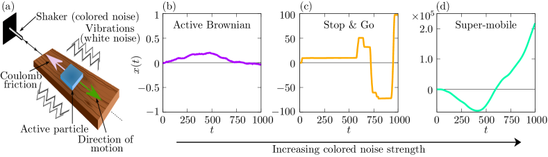
Figure 1: Coulomb friction-induced anomalous dynamical states. (a) Experimental realization of an active dynamics with Coulomb friction: The supporting plate is propelled by a shaker with a programmed protocol of colored noise, replicating the active force. Combined with the random vibrations of the supporting plate (white noise), it induces motion subjected to Coulomb friction. (b)-(d) Particle trajectories for different colored noise strength (activities), exploring the active Brownian state (b) for $f_{0}=0.1$, the Stop & Go state (c) for $f_{0}=1$, and the super-mobile dynamical state (d) for $f_{0}=10$. The other parameters of the simulations are $\tau_{0}=100$, $\Delta_{0}=1$, $v_{0}=0.1$.

Friction [1] has been studied by using empirical models starting from pioneering observations that date back to 350 A.D. (Themistius) “it is easier to further the motion of a moving body than to move a body at rest”. This qualitative discovery was systematically investigated by Coulomb in 1785 who noted that dry friction force depends only on the velocity direction. He developed the celebrated Coulomb’s friction law [2] which has proven to be fundamental on the macroscopic level [3, 4]. A huge further step in the study of dry friction at the molecular level was done by de Gennes, who explored its properties for Brownian motion [5] and suggested an experimental realization [6]. The research of de Gennes has prompted further theoretical [7, 8, 9, 10] and experimental investigations in the context of passive granular particles [11, 12], Brownian motors [13, 14, 15, 16], and the piston problem [17, 18].

Here, we consider active particles governed by Coulomb friction. The motion of these particles is self-sustained by an activity which acts as a non-equilibrium driving force with a stochastic evolution [19, 20, 21]. Thereby the active particles continuously inject energy into the system which is partially transformed into motion (kinetic energy) and partially irreversibly dissipated in the environment due to friction [22, 23]. For wet systems [24, 25], such as active colloids and bacteria, the friction is typically linear in the velocity [26, 27] due to the liquid solvent, originating from Stokes’ law [28]. By contrast, in dry systems, such as robots and active granular particles [29, 30, 31, 32, 33, 34, 35, 36], friction is generated by the contact with the ground. In this case, dynamics are governed by Coulomb friction which is almost insensitive to velocity [27]. We propose a minimal model of one-dimensional active motion with Coulomb friction, which shows intriguing features that have no counterpart in the case of Stokes friction. By increasing the amplitude of active force, we switch from the standard active Brownian motion dominated by white noise (Fig. 1 (b)) to a different dynamical “Stop & Go” regime (Fig. 1 (c)), which alternates diffusive behavior to running, accelerated motion. Further activity values induce an additional dynamical regime where the particle uniquely moves with an accelerated “super-mobile” motion (Fig. 1 (d)). A possible setup for studying active motion with Coulomb friction consists of an object (particle) resting on a horizontal, vibrating plate, connected to a shaker (Fig. 1(a)). The shaker is programmed to produce colored noise so that the active force acting on the particle is reproduced. This ingredient, combined with the random vibrations of the plate (white noise), induces the active motion of the particle, while the solid plate exerts on the particle a friction force that follows the Coulomb’s friction law.

Coulomb friction is modeled as a force which has a two components: A dynamic one, which decelerates an object already in motion, and a static one, which impedes the motion. The dynamic part does not depend on velocity, while the static part contributes for vanishing velocity $v$, making it more difficult to set the stationary object in motion. The friction force strength is set by two friction coefficients, which intrinsically depend on the material properties and are different for static and dynamic cases. Here, we consider the friction force, $\sigma(v)$ described by the Tustin empirical model [37]:

$$\sigma(v)=\Delta_{C}\operatorname*{sign}(v)\left[1+\frac{\Delta_{S}-\Delta_{C}}{\Delta_{C}}e^{-\frac{|v|}{v_{s}}}\right]\,,$$ (1)

where $\Delta_{C,S}$ are the Coulomb dynamic and static friction coefficients, respectively, with $\Delta_{S}\geq\Delta_{C}$. The term $v_{s}$ is the Stribeck velocity that sets the sharpness of $\sigma(v)$ for $v\to 0$ [38]. Expression (1) provides a minimal description for studying dynamic and static Coulomb friction in the particle equation of motion. Previously, theoretical analysis has mainly centered around the simpler scenario of purely dynamical friction $\Delta_{C}=\Delta_{S}$. In de Gennes’ original paper, emphasis was placed on velocity autocorrelation [5], while Touchette et al. provided the exact solution [7]. More recent studies have been obtained for colored noise with weak memory [39].

The dynamics of an inertial active particle with mass $m$ with friction force $\sigma(v)$, is minimally modeled as a one-dimensional Langevin equation for the particle velocity $v(t)=\dot{x}(t)$,

$$m\dot{v}(t)=-\sigma(v(t))+\sqrt{2K}\xi(t)+n(t)f\,.$$ (2)

Here, $t$ is time, and $K$ is the noise strength of the Gaussian white noise $\xi(t)$, characterized by zero average and unit variance. The time-dependent term $n(t)f$ represents the active force that drives the motion, where $f$ is the activity and the stochastic process $n(t)$ is chosen as an Ornstein-Uhlenbeck process with typical autocorrelation time $\tau$ and dynamics

$$\dot{n}(t)=-\frac{n(t)}{\tau}+\sqrt{\frac{2}{\tau}}\eta(t)\,.$$ (3)

In this equation, $\eta(t)$ is Gaussian white noise with zero average and unit variance. Such a choice for the active force corresponds to the active Ornstein-Uhlenbeck particle dynamics [40, 41, 42, 43, 44, 45, 46, 47].

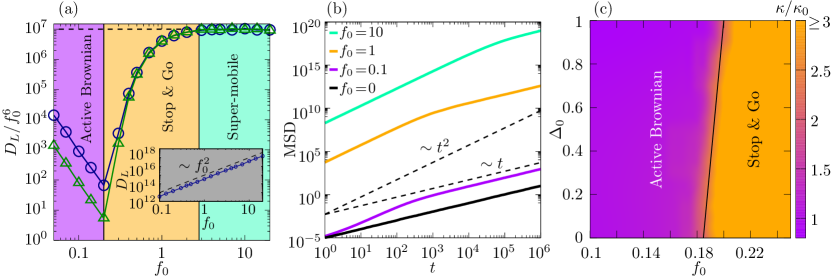
Figure 2: Stop & Go and super-mobile states. (a) Long-time time diffusion coefficient $D_{L}$ rescaled by $f_{0}^{6}$ as a function of $f_{0}$, with $\Delta_{0}=0$ (blue circles), and $\Delta_{0}=1$ (green triangles). The region of parameters corresponding to the Brownian regime, Stop & Go, and super-mobile regimes are colored in violet, yellow, and green, respectively, while the transitions are marked with vertical lines. In the inset, we show the diffusion coefficient in the absence of dry friction scaling as $\sim f_{0}^{2}$. (b) Mean squared displacement (MSD) $\langle((x(t)-(x(0))^{2}\rangle$, as a function of time, $t$, for different values of $f_{0}$ in the three dynamical states with $\Delta_{0}=0$. Here, dashed black lines denote the ballistic and diffusive time-scaling. Colors have the same ordering as the $\operatorname*{MSD}$ profiles. (c) State diagram in the plane of activity $f_{0}$ and relative friction coefficient $\Delta_{0}$. The color gradient shows the smoothed excess kurtosis, normalized with the value for the passive system. The black solid line indicates the crossover from active Brownian and Stop & Go dynamical states. The other parameters of the simulations are: $v_{0}=0.1,\;\tau_{0}=100$.

In what follows, we use $\Delta_{C}$, $\sqrt{\tau K}/\Delta_{C}$, $\tau K/m\Delta_{C}$ as units of force, time, and length, respectively. With this choice, the system is characterized by four dimensionless parameters (See Supplemental Material (SM) ): the reduced activity $f_{0}=f/\Delta_{C}$, which quantifies the active force effect compared to friction; the reduced noise strength $1/\tau_{0}=\sqrt{K/\tau}/\Delta_{C}$, which determines the impact of the noise kicks on the particle evolution; two friction parameters, i.e. the relative magnitude of the static and dynamic friction force $\Delta_{0}=\Delta_{S}/\Delta_{C}-1$ and the rescaled Stribeck velocity $v_{0}=mv_{s}/\sqrt{\tau K}$. We set $v_{0}=0.1$ since static friction has to affect the dynamics only for small velocity, and low noise strength $1/\tau_{0}=10^{-2}$, as usual in experimental active systems. In addition, the latter choice emphasizes the effect of activity and static friction which are mainly explored here.

For small activity, the active force $nf_{0}$ cannot exceed the friction force value on average and, thus, its dynamic effect is suppressed. The resulting motion is similar to the one shown by standard active particles. Indeed, intuitively, the active force induces an effective dry friction coefficient which is smaller (larger) than $\Delta_{C}$ if the active force and the velocity have the same (opposite) sign. Therefore, the characteristic trajectory of this Coulomb-driven active Brownian dynamical state is not qualitatively different from the usual regime displayed by an active particle (Fig. 1 (b)).

As the activity $f_{0}$ is increased, the active force $n\,f_{0}$ is more likely to exceed the friction force value in some time interval. When this happens, the trajectory displays fast acceleration in some time windows (here the particle “Goes”). These regimes are suppressed when, by fluctuations, the active force is smaller than the Coulomb friction: when this happens, the particle behaves as a Brownian particle as observed for small $f_{0}$ (here the particle “Stops”). This Stop & Go behavior can be directly observed in the particle trajectory (Fig. 1 (c)). A further increase of $f_{0}$ allows the active force to permanently exceed the friction force, except for the small time window when $nf_{0}$ reverses its direction. In this state, the friction mechanism is ineffective in hindering the motion except when the activity reverses. This results in a different regime characterized by super-mobile behavior, where the particle continuously accelerates and suddenly decelerates to reverse its motion (Fig. 1 (d)).

To characterize these three dynamical states, we investigate the long-time diffusion coefficient $D_{L}$ extracted from the mean-square displacement (MSD) $\langle\left(x(t)-x(0)\right)^{2}\rangle$. Independently of the activity and Coulomb friction coefficients, this observable shows a small-time ballistic regime $\langle\left(x(t)-x(0)\right)^{2}\rangle\sim t^{2}$ (Fig. 2 (a)), which is purely induced by the activity as usual for active particles [49, 50]. In the long-time regime, the $\operatorname*{MSD}$ approaches a diffusive behavior $\sim t$, which is due to the random change of the active force direction present in all the dynamical states. From here, we can extract the long-time diffusion coefficient $D_{L}$ that is reported as a function of $f_{0}$ for vanishing ($\Delta_{0}=0$) and non-vanishing static friction ($\Delta_{0}>0$). For small values of $f_{0}$ corresponding to the Brownian regime, $D_{L}$ scales as $f_{0}^{2}$, as expected for standard active Brownian particles (inset in Fig. 2 (a)). When the Stop & Go regime is approached, $D_{L}$ starts increasing faster with $f_{0}$. This anomalous scaling is due to the “Go” regimes which allows the particle to further explore the surrounding space. When “Stop” events are suppressed because of the large $f_{0}$ value, a scaling $D_{L}\sim f_{0}^{6}$ is reached in correspondence with the super-mobile state (Fig. 2 (a)).

The relative amplitude of static and dynamic friction $\Delta_{0}$ affects the diffusion properties only in the active Brownian regime by decreasing $D_{L}$, while it leaves almost unchanged Stop & Go and super-mobile states. This is because static friction plays a negligible role compared to dynamical friction during a Go state, since $|v|\gg v_{0}$ and thus $\sigma(v)\approx\Delta_{C}\operatorname*{sign}(v)$. However, we intuitively expect that an increase of the static friction, via $\Delta_{0}$, could affect the transition line from Brownian to the Stop & Go regime. To further characterize the role of $\Delta_{0}$, we focus on the steady-state velocity properties. Indeed, during “Go” states the velocity gains large values which is represented by the long tails of the velocity distribution which we quantify by studying its fourth moment. Specifically, we focus on the excess kurtosis, i.e. the deviation of the fourth velocity moment from the Gaussian value, $\kappa=\langle v^{4}\rangle/\langle v^{2}\rangle^{2}-3$. We normalize this observable with the excess kurtosis, $\kappa_{0}$, of a passive particle ($f_{0}=0$) so that $\kappa/\kappa_{0}$ reads $\approx 1$ in the active Brownian regime and assumes values $\gg 1$ in the Stop & Go state. Our analysis as a function of $f_{0}$ and $\Delta_{0}$ (Fig. 2 (c)) reveals that static friction $\Delta_{0}>0$ hinders the transition to the Stop & Go regime. Indeed, in this case, the active force needs to exceed a larger total dry friction to induce acceleration.

To further shed light on the effect of activity $f_{0}$ and static friction $\Delta_{0}$, we numerically and theoretically analyze the velocity distribution $p(v)$. As we expect from the kurtosis analysis, this observable does not show remarkable differences between the active Brownian regime and the passive case, where $p(v)$ decays exponentially as $\propto e^{-\tau_{0}|v|}$. By resorting to path-integrals techniques [51] (see SM for details), the expression for $p(v)$ can be generalized for small activity $f_{0}\ll 1$ (active Brownian state) where the main contribution occurs for $|v|\ll 1$ and reads

$$p(v)\sim e^{-\tau_{0}\left(|v|(\Delta_{0}+1)-\frac{\Delta_{0}}{2v_{0}}v^{2}-\frac{f_{0}^{2}|v|^{3}}{4(\Delta_{0}+1)}+\mathcal{O}(v^{4})\right)}\,.$$ (4)

Here, static friction and activity roughly have the same effect providing small deviations from the exponential tails (Fig. 3(a)-(b)). By contrast, in the Stop & Go state for larger values of $f_{0}$, the full shape of the distribution is distorted (Fig. 3(a)). In particular, in the Stop & Go regime, the tails slowly decay to zero, while in the super-mobile state the distribution is nearly flat with a small peak for vanishing velocity.

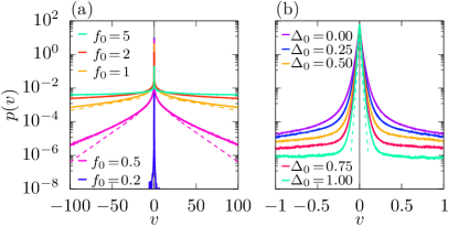
Figure 3: Velocity probability distribution. (a) probability distribution of the particle velocity $p(v)$ for $\Delta_{0}=0$ for various $f_{0}$; (b) $p(v)$ for $f=0.25$ for various $\Delta_{0}$. Dashed lines in panel (a) correspond to the analytical prediction given by Eq. (5), and dashed lines in panel (b) correspond to the analytical prediction given by Eq. (4) up to the first order. Colors have the same ordering as the density profiles. The other parameters of the simulations are: $v_{0}=0.1,\;\tau_{0}=100$.

Remarkably, our method is able to provide an analytical approximation for the velocity distribution $p(v)$ also for large activity $f_{0}$, where typically $|v|\gg 1$

$$p(v)\propto e^{-\frac{n_{\rm f}^{2}}{2}}\,.$$ (5a)

Here, $$n_{\rm f}$$ is set implicitly via the equation

$$2\tau_{0}\left[n_{\rm f}f_{0}-\ln(n_{\rm f}f_{0})-1\right]=v,\ n_{\rm f}>\frac{1}{f_{0}}\,.$$ (5b)

Equation (5) holds in the absence of static friction $\Delta_{0}=0$, while the full expression for $\Delta_{0}>0$ is reported in the SM. However, in agreement with the previous analysis, static friction provides a negligible contribution on $p(v)$ for $|v|\gg 1$.

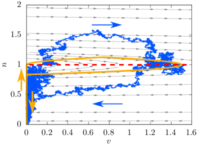
Figure 4: Typical trajectory in the Stop & Go regime. Escape-and-return particle trajectory in the plane of velocity $v$ and $n$. The blue line is obtained from numerical simulations, while the smooth orange one by integrating Eq. (6). Grey thin arrows are the force field given by Eqs. (2)-(3), while the red dashed horizontal line corresponds to the threshold activity level, such that $n=1/f_{0}$. The parameters of the simulation are: $f_{0}=1$, $\Delta_{0}=0$, $v_{0}=0.1,\;\tau_{0}=100$.

Our theoretical approach allows us to predict the typical escape particle trajectory, shown with a blue line in Fig. 4, by expressing $v$ as a function of $n$ (see SM for the details):

$$\frac{\differential v}{\differential n}=\mp\frac{\operatorname*{sign}(v)\tau_{0}}{n}\left[1+\Delta_{0}e^{-\frac{|v|}{v_{0}}}\right]\pm f_{0}\tau_{0}\,.$$ (6)

The two solutions imply that the particle displays a hysteresis-like trajectory in the $(n,v)$-plane, shown with an orange line in Fig. 4. An active particle, initially placed at $v=0$, $n=0$, maintains zero velocity until the active force exceeds the friction, i.e. at the threshold value such that $|v|=nf_{0}=1$.

From here, the particle starts accelerating (upper sign in Eq. (6)) and reaches a maximum velocity when the activity decreases below the threshold value. At this point, the particle slows down and relaxes to its initial state (lower sign in Eq. (6)). This hysteresis-like trajectory is a visualization of the Stop & Go regime and is purely induced by dry friction. Indeed, this behavior cannot be achieved by active dynamics governed by Stokes viscous forces for which $v\propto n$.

The fundamental emergence of the three dynamic states, rooted in the interplay between active and Coulomb friction force, suggests their existence in a broader range of experimental systems beyond the proposed setup. Good candidates are Hexbug particles [52, 53, 54, 55, 56] or sliding robots [57], which are activated by internal motors and placed on a surface whose material properties can be suitably tuned to enhance Coulomb friction. Alternatively, activity can be induced on any granular object via programmed shakers that produced colored noise [58, 59, 60, 36]. The emerging Stop & Go and super-mobile states can pave the way towards the development of intriguing applications in active granular matter. Super-mobile active granulates are applicable for efficient spatial exploration and food search, by taking advantage of the enhanced diffusion properties caused by the anomalous scaling of the long-time diffusion coefficient with the activity. The dynamical transitions shown here could lead to unprecedented collective phenomena for active systems giving rise to giant density fluctuations as well as density waves and pulsating clusters.

Acknowledgement. AA, CS and HL acknowledge the financial support by Deutsche Forschungsgemeinschaft (German Research Foundation), Project LO 418/25-1. LC acknowledges the European Union MSCA-IF fellowship for funding the project CHIAGRAM.

In this Supplemental Material, we provide details on the numerical study and the dimensionless parameters for the dynamics of an active particle subject to static and dynamic Coulomb friction. In addition, we derive the theoretical predictions (Eqs. (4)-(6)) reported in the main text and discuss the method employed and the approximation involved.

I Details of the numerical study

In this section, we provide additional details on the numerical implementation of the equation of motion for an active particle subject to static and dynamic Coulomb friction by specifically discussing its dimensionless form.

The dynamics of an active particle with Coulomb friction (Eqs. (2)-(3) of the main text), reads

$$m\dot{v}(t)= -\sigma(v(t))+\sqrt{2K}\xi(t)+n(t)f,$$ (S1a)

$$\dot{n}(t)= -\frac{n(t)}{\tau}+\sqrt{\frac{2}{\tau}}\eta(t)\,,$$ (S1b)

with

$$\sigma(v)=\Delta_{C}\operatorname*{sign}(v)\left[1+\frac{\Delta_{S}-\Delta_{C}}{\Delta_{C}}e^{-\frac{|v|}{v_{s}}}\right].$$ (S2)

We consider $\tau K/(m\Delta_{C})$ as a unit of length to rescale the particle position, $\sqrt{\tau K}/\Delta_{C}$ as a unit of time, and $\Delta_{C}$ as a unit of force, i.e.

$$x\rightarrow\tau K/(m\Delta_{C})x,$$ (S3a)

$$t\rightarrow\sqrt{\tau K}/\Delta_{C}t,$$ (S3b)

$$\sigma(v)\rightarrow\Delta_{C}\sigma(v)\,.$$ (S3c)

In this way, rescaled position, time and force are dimensionless and the corresponding dynamics read

$$\dot{v}(t)=-\sigma(v(t))+\sqrt{\frac{2}{\tau_{0}}}\xi(t)+n(t)f_{0},$$ (S4a)

$$\dot{n}(t)=-\frac{n(t)}{\tau_{0}}+\sqrt{\frac{2}{\tau_{0}}}\eta(t),$$ (S4b)

$$\sigma(v)=\operatorname*{sign}(v)\left[1+\Delta_{0}e^{-\frac{|v|}{v_{0}}}\right],$$ (S4c)

Here, the system is controlled by four dimensionless parameters:

1. the parameter $f_{0}=f/\Delta_{C}$, i.e. the rescaled activity, quantifies the effect of the active force compared to friction. For $f_{0}\gg 1$, the active force has a stronger impact compared to friction, while for $f_{0}\ll 1$ friction dominates over the active forces. In the numerical study, $f_{0}$ is systematically changed, exploring both small and large activity regimes.

2. the noise strength $1/\tau_{0}=\sqrt{K/\tau}/\Delta_{C}$, which determines the impact of the noise kick in the dynamics. This parameter is kept fixed in numerical simulations $1/\tau_{0}=10^{-2}$ because it is usually small in active systems. In addition, in the opposite regime, for $1/\tau_{0}\gg 1$, the role of the active force is hindered. We remark that $\tau_{0}$ plays the role of an inverse temperature.

3. $\Delta_{0}=\Delta_{S}/\Delta_{C}-1$ represents the relative magnitude of the static and dynamic friction force. For $\Delta_{0}=0$, the dynamics is only governed by dynamic friction, while for $\Delta_{0}>0$ also static friction takes place. In numerical simulations, we explore the effect of $\Delta_{0}$ to understand the impact of static friction of our results.

4. the rescaled Stribeck velocity $v_{0}=mv_{s}/\sqrt{\tau K}$ determines the shape of the friction curve near zero velocities. The limit $v_{0}\to 0$ implies that static friction is significant only at vanishing velocity when the particle does not move while increasing $v_{0}$ extends the relevance of the friction force to slowly moving particles. This parameter is chosen as $v_{0}=0.1$ in numerical simulations.

II Theoretical Prediction

In this section, we derive the theoretical predictions, Eq. (4) and Eqs. (5) of the main text, holding for small and large velocities, respectively. At first, we provide a general explanation of the method which is then applied to an active particle subject to Coulomb friction, considering both the system with vanishing and non-vanishing static friction.

The system dynamics, described by the dimensionless dynamics (S4), can be expressed in a compact form by defining the vector $q(t)$ with components $(v(t),n(t))$. In this way, for $i$ representing coordinates $v$ and $n$, we obtain

$$\dot{q}_{i}(t)=-f_{i}(q(t))+\sqrt{\frac{2}{\tau_{0}}}\xi_{i}(t)\,,$$ (S5)

where the general force fields $f_{i}$ read

$$f_{v}= \operatorname*{sign}(v)\left[1+\Delta_{0}e^{-\frac{|v|}{v_{0}}}\right]-nf_{0},$$ (S6a)

$$f_{n}= \frac{n}{\tau_{0}}\,.$$ (S6b)

To develop our theoretical argument, we consider the transition probability $\displaystyle\mathcal{P}(q_{f},T|q_{0},0)$ between the initial state $q(0)=(n(0),v(0))$ at time $t=0$ and the final state $q(T)=(n(T),v(T))$ at time $t=T$. This probability can be expressed by using the path integral formalism:

$$\mathcal{P}(q_{f},T|q_{0},0)=\int\limits_{q(0)=q_{0}}^{q(t)=q_{f}}\mathcal{D}q(t)e^{-\tau_{0}S[q(t)]},$$ (S7)

where

$$S[q(t)]=\frac{1}{4}\sum_{i}\int_{0}^{T}\left(\dot{q}_{i}(t)+f_{i}(q(t))\right)^{2}\differential t+\mathcal{O}(\tau_{0}^{-1})$$ (S8)

is the Onsager-Machlup functional [1].

Let us first fix only the final velocity $v(T)=v_{f}$ and leave $n(T)$ floating. In what follows we assume that $v_{f}>0$, however, this choice is optional due to translation symmetry $v\to-v$ of Eqs. (S4). Since the meaning of the Onsager-Machlup functional is similar to the Lagrangian of the classical system [2], by using analogy with the classical mechanics we can say that this functional sets the dynamical equation of motion that defines the manifold of escape paths, and the most probable escape path additionally obeys the global minimization over $n(T)$. The optimizing path that minimizes the functional satisfies the Euler-Lagrange equation,

$$\dot{q}_{i}(t)+f_{i}(q(t))=2p_{i}(t),$$ (S9a)

where we have introduced the analog of classical momentum as

$$\dot{p}_{i}(t)-p_{j}\partial_{i}f_{j}(q(t))=0\,.$$ (S9b)

The classical analog of the Hamiltonian corresponding to Eqs. (S9) is given by

$$H(p,q;t)=\sum_{i}\left[p_{i}^{2}(t)-f_{i}(q(t))p_{i}(t)\right]\,.$$ (S10)

We remark that Eqs. (S9) can be derived by implementing the Wentzel–Kramers–Brillouin (WKB) method to the Fokker-Planck equation corresponding to the Langevin dynamics [3].

The Hamilton equations (S9) have the first integral $\mathcal{E}=H(p,x;t)$. By combining (S9a), (S10), we can rewrite it as

$$\mathcal{E}=\frac{1}{4}\sum_{i}\left[\dot{q}_{i}^{2}(t)-f_{i}^{2}(q(t))\right]=\rm C\,,$$ (S11)

where $\rm C$ is a constant term. The probability in Eq. (S7) reads

$$\mathcal{P}(q_{f},T|q_{i},0)\Big{|}_{T\to\infty}=P(q_{f})\propto e^{-\tau_{0}S(q_{f})}\,,$$ (S12)

where $S$ is the analog of the classical action and can be calculated by applying the Maupertius principle [4],

$$S=\sum_{i}\int\limits_{0}^{T}p_{i}(t)\dot{q}_{i}(t)\differential t-\mathcal{E}t=\sum_{i}\int_{\rm traj}p_{i}\differential q_{i}-\mathcal{E}t\,,$$ (S13)

where $\int_{\rm traj}$ is the integral over the trajectory of $q$. Alternatively, if we are only interested in the shape of the trajectory, we can rewrite it as

$$S= \hskip 3.01385pt\mathcal{E}t+\frac{1}{2}\sum_{i}\int\limits_{0}^{T}\differential t(f_{i}^{2}(q(t))+f_{i}(q(t))\dot{q}_{i}(t))$$

$$= \hskip 3.01385pt\frac{1}{2}\int_{\rm traj}\left\{\sqrt{(4\mathcal{E}+\sum_{i}f_{i}^{2}(q(t)))\sum_{i}\differential q_{i}\differential q_{i}}+\sum_{i}\left[f_{i}(q(t))\differential q_{i}\right]\right\}.$$ (S14)

Since our interest is the steady-state distribution (S12), in what follows, we consider $T\to\infty$, corresponding to $\mathcal{E}=0$ [3].

II.1 Theoretical prediction for large v, with vanishing static dry friction

For a particle subject to static and dry friction with the force field (S6), Hamilton equations correspond to four equations, for velocity $v$, stochastic process $n$, and the corresponding conjugate momenta, $p_{v}$ and $p_{n}$, respectively:

$$\dot{v} = \frac{2p_{v}}{\tau_{0}}-\operatorname*{sign}(v)\left[1+\Delta_{0}e^{-\frac{|v|}{v_{0}}}\right]+nf_{0},$$ (S15a)

$$\dot{n} = 2p_{n}-\frac{n}{\tau_{0}},$$ (S15b)

$$\dot{p}_{v} = p_{v}\left[2\delta(v)(1+\Delta_{0})-\frac{\Delta_{0}}{v_{0}}e^{-\frac{|v|}{v_{0}}}\right],$$ (S15c)

$$\dot{p}_{n} = \frac{p_{n}}{\tau_{0}}-p_{v}f_{0}\,,$$ (S15d)

where $\delta(v)$ is a Dirac delta function obtained from the derivative of $\operatorname*{sign}(v)$. Those dynamical equations are not solvable in quadratures due to the discontinuity in the friction force profile so that this global minimization can be performed only numerically. We therefore reformulate the question about the velocity distributions: which factor, noise or activity, exerts greater impact when the object acquires velocity? In the considered case of low noise the answer is that for attaining small velocities near zero, noise plays the predominant role, similar to the passive case where noise is the sole mechanism initiating movement. For the larger velocities, this is no longer the case since activity emerges as the primary contributing factor. With this understanding, we can approximate global minimization through constrained minimization. The constraint is that the action gained along one of the axes is negligible, depending on which mechanism dominates in velocity gaining. For $v_{f}\gg 1$ the dominant mechanism is activity, so the action is zero along $v$-axis. Using the corresponding ansatz $p_{v}=0$, we obtain two solutions of Eqs. (S15d), one of which corresponds to the escape part of the trajectory path,

$$\dot{v} =-\operatorname*{sign}(v)\left[1+\Delta_{0}e^{-\frac{|v|}{v_{0}}}\right]+nf_{0},$$ (S16a)

$$\dot{n} =p_{n}=\frac{n}{\tau_{0}},$$ (S16b)

$$p_{v} =0\,,$$ (S16c)

and another corresponding to the relaxation part (gradient-path):

$$\dot{v} =-\operatorname*{sign}(v)\left[1+\Delta_{0}e^{-\frac{|v|}{v_{0}}}\right]+nf_{0},$$ (S17a)

$$\dot{n} =-\frac{n}{\tau_{0}},$$ (S17b)

$$p_{v} =p_{n}=0\,.$$ (S17c)

We note that the return part is always given by $p_{n}=p_{v}=0$, as this is the solution for the generic form of Hamilton equations (S9). At the same moment, this return part also does not contribute to probability Eqs. (S12), as the corresponding contribution in (S13) is equal to zero [3].

Since we are interested only in the trajectory shape, we rewrite Eqs. (S16), (S17) as

$$\frac{\differential v}{\differential n}=\mp\frac{\operatorname*{sign}(v)\tau_{0}}{n}\left[1+\Delta_{0}e^{-\frac{|v|}{v_{0}}}\right]\pm f_{0}\tau_{0},$$ (S18)

with upper sign corresponding to escape part (S16), and lower sign corresponding to return part (S17).

Let us first consider $\Delta_{0}=0$. The trajectory consists of 4 parts. Initially, in the first part, activity increases according to Eq. (S16b), while velocity remains constant at zero. Subsequently, during the second part, velocity begins to increase when $n>1/f_{0}$, driven by the positive acceleration $\dot{v}$ in Eq. (S16a). The switch to the third part occurs when the escape trajectory switches to the return trajectory at $n=n_{\rm f}$, where $n_{\rm f}$ is implicitly determined by the maximum velocity $v_{f}$ attained. During this part, activity starts to decline according to Eq. (S17b), yet the particle continues to accelerate until the point when $\dot{v}=0$ as described in Eq.(S17a) for $n=1/f_{0}$. Following this, the particle decelerates, eventually reaching zero velocity at $n=n_{\rm a}$. Following that, in the fourth part, velocity remains at 0 while activity relaxes to 0 as well. In summary:

$$v(n)=\begin{cases}0,\ n\in[0;\frac{1}{f_{0}}[,\\ \tau_{0}\left[nf_{0}-\ln(nf_{0})-1\right],\ n\in[\frac{1}{f_{0}};n_{\rm f}[,\\ v_{f}-\tau_{0}\left[nf_{0}-\ln(nf_{0})-1\right],\ n\in[n_{\rm f};n_{\rm a}[,\\ 0,\ n\in[n_{\rm a};0[.\end{cases}$$ (S19)

with

$$2\tau_{0}\left[n_{\rm f}f_{0}-\ln(n_{\rm f}f_{0})-1\right]=v_{f},\ n_{\rm f}>\frac{1}{f_{0}},$$ (S20)

$$\tau_{0}\left[n_{\rm a}f_{0}-\ln(n_{\rm a}f_{0})-1\right]=v_{f},\ n_{\rm a}<\frac{1}{f_{0}}\,.$$ (S21)

Combining (S12), (S13), (S16), (S17), we obtain

$$p(v_{f})\propto e^{-\frac{n_{\rm f}^{2}(v_{f})}{2}}\,.$$ (S22)

with $n_{\rm f}$ depending on $v_{f}$ implicitly via Eq. (S20). Equation (S22) corresponds to Eqs. (5) of the main text.

II.2 Theoretical prediction for large v, with static dry friction

Solving Eq. (S18) for $\Delta_{0}\neq 0$ is less trivial. Due to the nature of the static friction, here motion starts for activity $n=1/f_{0}(1+\Delta_{0})$. Since then friction decreases for higher velocity, this activity is a priori enough to reach a certain velocity (which can be also larger than $v_{f}$), even if the escape part switches to return immediately after the initiation of motion. The activity corresponding to the maximum velocity $v_{\rm max}$ is obtained from Eq. (S17a) for $\dot{v}=0$. Solving Eq. (S18) before these conditions, we obtain

$$v(n)=\begin{cases}0,&\text{if }n\in\left[0,\frac{1+\Delta_{0}}{f_{0}}\right[,\vspace{.4ex}\\ \vspace{.4ex}v_{e}(n),&\text{if }n\in\left[\frac{1+\Delta_{0}}{f_{0}},n_{\rm f}\right[,\ v_{e}\left(\frac{1+\Delta_{0}}{f_{0}}\right)=0,\\ v_{r}(n),&\text{if }n\in[n_{\rm f},n_{\rm a}[,\ v_{r}(n_{\rm a})=0,\ v_{r}\left(\frac{1+\Delta_{0}e^{-\frac{v_{f}}{v_{0}}}}{f_{0}}\right)=v_{\rm max},\\ 0,&\text{if }n\in[n_{\rm a},0[.\end{cases}$$ (S23)

where escape and return parts $v_{e,r}(n)$ read

Here, $E_{n}(x)=x^{n}\Gamma(1-n,x)$ is the exponential integral, with $\Gamma(a,x)=\int_{x}^{\infty}t^{a-1}e^{-t}\differential t$ being the incomplete Gamma-function.

As we have mentioned before, for static friction during the initiation of motion, the particle gains (at least) some velocity $v_{\rm min}$ in any case. It is derived from the condition of instantaneous transition from escape to return at the moment of initiation and is defined by the formula:

$$v_{\rm min}=-f_{0}\tau_{0}+\ v_{0}\ln\left[e^{\frac{\tau_{0}\left(f_{0}+\Delta_{0}f_{0}-\ln(1+\Delta_{0})\right)}{v_{0}}}+\frac{\Delta_{0}\tau_{0}\left(E_{1+\frac{\tau_{0}}{v_{0}}}\left(-\frac{f_{0}\tau_{0}}{v_{0}}\right)\right)-\left\{-\frac{\tau_{0}f_{0}}{v_{0}}\right\}^{\frac{\tau_{0}}{v_{0}}}\Gamma\left(-\frac{\tau_{0}}{v_{0}},\frac{-f_{0}\tau_{0}(1+\Delta_{0})}{v_{0}}\right)}{v_{0}}\right].$$ (S24)

Thus, the maximum velocity gained during the escape is the greater of $v_{\rm min}$ and the pre-set $v_{f}$:

$$v_{\rm max}=\max\left\{v_{\rm min},v_{f}\right\}$$ (S25)

The probability distribution is obtained identically to Eq. (S22), with $n_{\rm f}$ now depending implicitly on $v_{f}$ via Eq. (S23).

II.3 Theoretical prediction for small v

For noise-induced velocities $v_{f}\ll 1$, the analogous ansatz $p_{n}=0$ is not helpful for the solution for the escape part. Therefore, we make another assumption using a similar idea: we assume that $n_{\rm f}$ in the final state $q_{f}$ which minimizes the action is small, $n_{\rm f}\ll 1$, and that the trajectory connecting initial and final state is a line. As a consequence, this trajectory can be parameterized as $n=\alpha v$. The action is then minimized if the angle $\alpha_{0}$ fulfills the following minimization condition:

$$\frac{\partial S}{\partial\alpha}\Big{|}_{\alpha=\alpha_{0}}=0,$$ (S26)

so that Eq. (S14) then reads:

$$S=\frac{1}{2}\int\limits_{0}^{v_{f}}\left\{\sqrt{\left[(1+\Delta_{0}e^{-\frac{v}{v_{0}}}-\alpha vf_{0})^{2}+\frac{\alpha^{2}v^{2}}{\tau_{0}^{2}}\right](\alpha^{2}+1)}+(1-\alpha vf_{0})+\frac{\alpha^{2}v}{\tau_{0}}\right\}\differential v\,.$$ (S27)

As this integral cannot be integrated analytically, we calculate it as Maclaurin series for small $n_{\rm f},v_{f}$. In this limit, the angle $\alpha_{0}$ minimizing this action is

$$\alpha_{0}=\frac{v_{f}f_{0}}{1+\Delta_{0}}+\mathcal{O}(v_{f}^{2})\,.$$ (S28)

By calculating action for this $\alpha_{0}$ and substituting it to Eq. (S12), we obtain an expression for the velocity distribution $p(v)$ holding for $|v|\ll 1$:

$$p(v)\propto e^{-\tau_{0}\left(|v|(\Delta_{0}+1)-\frac{\Delta_{0}}{2v_{0}}v^{2}-\frac{f_{0}^{2}|v|^{3}}{4(\Delta_{0}+1)}+\mathcal{O}(v^{4})\right)}\,.$$ (S29)

Equation (S29) corresponds to the prediction (4) of the main text. In agreement with our intuition, we additionally observe that for small $v$, the expression for $p(v)$ differs from that of a passive particle subject to dry friction only for subdominant, third-order terms in power of $v$.

References

- Fall et al. [2014] A. Fall, B. Weber, M. Pakpour, N. Lenoir, N. Shahidzadeh, J. Fiscina, C. Wagner, and D. Bonn, Phys. Rev. Lett. 112, 175502 (2014).
- Coulomb [1821] C. A. Coulomb, Théorie des machines simples en ayant égard au frottement de leurs parties et à la roideur des cordages (Bachelier, 1821).
- Olsson et al. [1998] H. Olsson, K. J. Åström, C. C. De Wit, M. Gäfvert, and P. Lischinsky, Eur. J. Control 4, 176 (1998).
- Pennestrì et al. [2016] E. Pennestrì, V. Rossi, P. Salvini, and P. P. Valentini, Nonlinear Dyn. 83, 1785 (2016).
- de Gennes [2005] P.-G. de Gennes, J. Stat. Phys. 119, 953 (2005).
- Daniel et al. [2005] S. Daniel, M. K. Chaudhury, and P.-G. de Gennes, Langmuir 21, 4240 (2005).
- Touchette et al. [2010] H. Touchette, E. V. der Straeten, and W. Just, J. Phys. A: Math. Theor. 43, 445002 (2010).
- Chen and Just [2014a] Y. Chen and W. Just, Phys. Rev. E 89, 022103 (2014a).
- Lequy and Menzel [2023] T. Lequy and A. M. Menzel, Phys. Rev. E 108, 064606 (2023).
- Plati et al. [2023] A. Plati, A. Puglisi, and A. Sarracino, arXiv eprints (2023).
- Gnoli et al. [2013] A. Gnoli, A. Puglisi, and H. Touchette, Europhys. Lett. 102, 14002 (2013).
- Lemaître et al. [2021] A. Lemaître, C. Mondal, I. Procaccia, and S. Roy, Phys. Rev. B 103, 054110 (2021).
- Baule and Sollich [2012] A. Baule and P. Sollich, Europhys. Lett. 97, 20001 (2012).
- Chen and Just [2014b] Y. Chen and W. Just, Phys. Rev. E 90, 042102 (2014b).
- Manacorda et al. [2014] A. Manacorda, A. Puglisi, and A. Sarracino, Commun. Theor. Phys. 62, 505 (2014).
- Semeraro et al. [2023] M. Semeraro, G. Gonnella, E. Lippiello, and A. Sarracino, Symmetry 15, 200 (2023).
- Sarracino et al. [2013] A. Sarracino, A. Gnoli, and A. Puglisi, Phys. Rev. E 87, 040101 (2013).
- Sano and Hayakawa [2014] T. G. Sano and H. Hayakawa, Phys. Rev. E 89, 032104 (2014).
- Marchetti et al. [2013] M. Marchetti, J. Joanny, S. Ramaswamy, T. Liverpool, J. Prost, M. Rao, and R. A. Simha, Rev. Mod. Phys. 85, 1143 (2013).
- Elgeti et al. [2015a] J. Elgeti, R. G. Winkler, and G. Gompper, Rep. Prog. Phys. 78, 56601 (2015a).
- Bechinger et al. [2016] C. Bechinger, R. Di Leonardo, H. Löwen, C. Reichhardt, G. Volpe, and G. Volpe, Rev. Mod. Phys. 88, 045006 (2016).
- O’Byrne et al. [2022] J. O’Byrne, Y. Kafri, J. Tailleur, and F. van Wijland, Nat. Rev. Phys. 4, 167 (2022).
- Fodor et al. [2021] É. Fodor, R. L. Jack, and M. E. Cates, Annu. Rev. Condens. Matter Phys. 13, 215 (2021).
- Zöttl and Stark [2016] A. Zöttl and H. Stark, J. Phys.: Condens. Matter 28, 253001 (2016).
- Löwen [2020] H. Löwen, J. Chem. Phys. 152, 040901 (2020).
- Romanczuk and Schimansky-Geier [2011] P. Romanczuk and L. Schimansky-Geier, Phys. Rev. Lett. 106, 230601 (2011).
- Romanczuk et al. [2012] P. Romanczuk, M. Bär, W. Ebeling, B. Lindner, and L. Schimansky-Geier, Eur. Phys. J. Spec. Top. 202, 1 (2012).
- Elgeti et al. [2015b] J. Elgeti, R. G. Winkler, and G. Gompper, Rep. Prog. Phys. 78, 056601 (2015b).
- Aranson et al. [2007] I. S. Aranson, D. Volfson, and L. S. Tsimring, Phys. Rev. E 75, 051301 (2007).
- Kudrolli et al. [2008] A. Kudrolli, G. Lumay, D. Volfson, and L. S. Tsimring, Phys. Rev. Lett. 100, 058001 (2008).
- Kumar et al. [2014] N. Kumar, H. Soni, S. Ramaswamy, and A. Sood, Nat. Commun. 5, 4688 (2014).
- Koumakis et al. [2016] N. Koumakis, A. Gnoli, C. Maggi, A. Puglisi, and R. Di Leonardo, New J. Phys. 18, 113046 (2016).
- Agrawal and Glotzer [2020] M. Agrawal and S. C. Glotzer, Proc. Natl. Acad. Sci. U.S.A. 117, 8700 (2020).
- Walsh et al. [2017] L. Walsh, C. G. Wagner, S. Schlossberg, C. Olson, A. Baskaran, and N. Menon, Soft Matter 13, 8964 (2017).
- Baconnier et al. [2022] P. Baconnier, D. Shohat, C. H. López, C. Coulais, V. Démery, G. Düring, and O. Dauchot, Nat. Phys. 18, 1234 (2022).
- Caprini et al. [2024] L. Caprini, A. Ldov, R. K. Gupta, H. Ellenberg, R. Wittmann, H. Löwen, and C. Scholz, Commun. Phys. 7, 52 (2024).
- Marton and Lantos [2007] L. Marton and B. Lantos, IEEE Trans. Ind. Electron. 54, 511 (2007).
- Stribeck [1902] R. Stribeck, Zeitschrift des Vereines Deutscher Ingenieure 46, 1341 (1902).
- Geffert and Just [2017] P. M. Geffert and W. Just, Phys. Rev. E 95, 062111 (2017).
- Szamel [2014] G. Szamel, Phys. Rev. E 90, 012111 (2014).
- Maggi et al. [2014] C. Maggi, M. Paoluzzi, N. Pellicciotta, A. Lepore, L. Angelani, and R. Di Leonardo, Phys. Rev. Lett. 113, 238303 (2014).
- Wittmann et al. [2017] R. Wittmann, C. Maggi, A. Sharma, A. Scacchi, J. M. Brader, and U. M. B. Marconi, J. Stat. Mech.: Theory Exp. 2017 (11), 113207.
- Caprini and Marconi [2018] L. Caprini and U. M. B. Marconi, Soft matter 14, 9044 (2018).
- Fily [2019] Y. Fily, J. Chem. Phys. 150, 174906 (2019).
- Woillez et al. [2020] E. Woillez, Y. Kafri, and N. S. Gov, Phys. Rev. Lett. 124, 118002 (2020).
- Martin et al. [2021] D. Martin, J. O’Byrne, M. E. Cates, É. Fodor, C. Nardini, J. Tailleur, and F. Van Wijland, Phys. Rev. E 103, 032607 (2021).
- Keta et al. [2022] Y.-E. Keta, R. L. Jack, and L. Berthier, Phys. Rev. Lett. 129, 048002 (2022).
- Note [1] See Supplemental Material [url] for details of analytical calculations, which includes Refs. [51, 61, 62, 63].
- ten Hagen et al. [2011] B. ten Hagen, S. van Teeffelen, and H. Löwen, J. Phys.: Condens. Matter 23, 194119 (2011).
- Caprini and Marini Bettolo Marconi [2021] L. Caprini and U. Marini Bettolo Marconi, J. Chem. Phys. 154, 024902 (2021).
- Caroli et al. [1981] B. Caroli, C. Caroli, and B. Roulet, J. Stat. Phys. 26, 83 (1981).
- Dauchot and Démery [2019] O. Dauchot and V. Démery, Phys. Rev. Lett. 122, 068002 (2019).
- Tapia-Ignacio et al. [2021] C. Tapia-Ignacio, L. L. Gutierrez-Martinez, and M. Sandoval, J. Stat. Mech.: Theory Exp. 2021 (5), 053404.
- Leoni et al. [2020] M. Leoni, M. Paoluzzi, S. Eldeen, A. Estrada, L. Nguyen, M. Alexandrescu, K. Sherb, and W. W. Ahmed, Phys. Rev. Res. 2, 043299 (2020).
- Horvath et al. [2023] D. Horvath, C. Slabỳ, Z. Tomori, A. Hovan, P. Miskovsky, and G. Bánó, Phys. Rev. E 107, 024603 (2023).
- Chen et al. [2023] L. Chen, K. J. Welch, P. Leishangthem, D. Ghosh, B. Zhang, T.-P. Sun, J. Klukas, Z. Tu, X. Cheng, and X. Xu, arXiv e-prints (2023).
- Hamon et al. [2010] P. Hamon, M. Gautier, and P. Garrec, in 2010 IEEE/RSJ International Conference on Intelligent Robots and Systems (2010) pp. 6187–6193.
- Kudrolli [2010] A. Kudrolli, Phys. Rev. Lett. 104, 088001 (2010).
- Deseigne et al. [2010] J. Deseigne, O. Dauchot, and H. Chaté, Phys. Rev. Lett. 105, 098001 (2010).
- Soni et al. [2020] H. Soni, N. Kumar, J. Nambisan, R. K. Gupta, A. Sood, and S. Ramaswamy, Soft Matter 16, 7210 (2020).
- Maslov and Fedoriuk [1981] V. P. Maslov and M. V. Fedoriuk, Semiclassical Approximation in Quantum Mechanics (Reidel, Dordrecht, 1981).
- Antonov et al. [2023] A. Antonov, A. Leonidov, and A. Semenov, Phys. Rev. E 108, 024134 (2023).
- Landau and Lifshitz [1976] L. D. Landau and E. M. Lifshitz, Mechanics. Vol. 1 (Butterworth-Heinemann, 1976).
Supplemental Material for

References

- Caroli et al. [1981] B. Caroli, C. Caroli, and B. Roulet, J. Stat. Phys. 26, 83 (1981).
- Maslov and Fedoriuk [1981] V. P. Maslov and M. V. Fedoriuk, Semiclassical Approximation in Quantum Mechanics (Reidel, Dordrecht, 1981).
- Antonov et al. [2023] A. Antonov, A. Leonidov, and A. Semenov, Phys. Rev. E 108, 024134 (2023).
- Landau and Lifshitz [1976] L. D. Landau and E. M. Lifshitz, Mechanics. Vol. 1 (Butterworth-Heinemann, 1976).