Uncovering Tidal Treasures: Automated Classification of Faint Tidal Features in DECaLS Data

Abstract

Tidal features are a key observable prediction of the hierarchical model of galaxy formation and contain a wealth of information about the properties and history of a galaxy. Modern wide-field surveys such as LSST and Euclid will revolutionise the study of tidal features. However, the volume of data will far surpass the capacity to inspect each galaxy to identify the feature visually, thereby motivating an urgent need to develop automated detection methods. This paper presents a visual classification of $\sim 2,000$ galaxies from the DECaLS survey into different tidal feature categories: arms, streams, shells, and diffuse. Using these labels, we trained a Convolutional Neural Network (CNN) to reproduce the assigned visual classifications. Overall our network performed well and retrieved a median $81.1^{+5.8}_{-6.5}$, $65.7^{+5.0}_{-8.4}$, $91.3^{+6.0}_{-5.9}$, and $82.3^{+1.4}_{-7.9}$ per cent of the actual instances of arm, stream, shell, and diffuse features respectively for just 20 per cent contamination. We verified that the network was classifying the images correctly by using a Gradient-weighted Class Activation Mapping analysis to highlight important regions on the images for a given classification. This is the first demonstration of using CNNs to classify tidal features into sub-categories, and it will pave the way for the identification of different categories of tidal features in the vast samples of galaxies that forthcoming wide-field surveys will deliver.

1 Introduction

Faint tidal features are a crucial observational tracer of hierarchical galaxy formation and evolution in the $\Lambda$CDM Universe. In this framework, galaxies grow in size and mass by accreting or merging with other galaxies (e.g. White & Rees, 1978; White & Frenk, 1991), these mergers are often described as being major (mass ratio of $\sim 0.1$ – 1) or minor (mass ratio $\lesssim 0.1$) (e.g. Davies et al., 2015; Hendel & Johnston, 2015). A significant proportion of a galaxy’s mass can originate from material accreted from other galaxies and, in particular, from minor mergers (e.g. Oser et al., 2010; Ownsworth et al., 2014) which are expected to be more common than major mergers (e.g. Fakhouri et al., 2010). Tidal features are the debris left behind by these interactions (e.g. Toomre & Toomre, 1972) either from recently accreted material from minor mergers or late-stage relics of majors. These features have various morphologies (e.g. Quinn, 1982) but are typically long-lived (e.g. Mancillas et al., 2019) and low surface brightness, with fewer features visible in shallower images (e.g. Johnston et al., 2008; Vera-Casanova et al., 2022).

Tidal features contain a wealth of information about a galaxy’s past. As tidal features are direct byproducts of galaxy mergers, it is possible to reconstruct the merger history of a galaxy by studying its tidal features (e.g. Johnston et al., 1999, 2008). In particular, the morphology of the tidal features can be connected to the stellar kinematics and formation history of the galaxy (e.g. Valenzuela & Remus, 2022) and can probe the orbital distribution of progenitor galaxies (e.g. Hendel & Johnston, 2015). Hence, there is interest in constraining the morphology of the tidal features, over and above generating a large sample where some kind of feature is present. Mergers and interactions have significant impacts on the stellar kinematics of galaxies (e.g. Yoon et al., 2022), and tidal stripping could be a considerable source of star formation suppression (e.g. Spilker et al., 2022). Tidal features can also be studied to give deeper insights into dark matter (e.g. Sanderson et al., 2015; Bovy et al., 2016; Pearson et al., 2022) and as tests of the cosmological model (e.g. Johnston et al., 2001; Conselice et al., 2014). However, to better understand this, it is necessary to build up a significant sample of identified tidal features, which requires probing deeper limiting surface brightnesses.

Forthcoming wide-field surveys, such as the Legacy Survey of Space and Time (LSST; Ivezić et al., 2019) at the Vera C. Rubin Observatory and the European Space Agency’s Euclid (Laureijs et al., 2011), will revolutionise the study of the low surface brightness Universe, including tidal features. These surveys will probe deep limiting surface brightnesses over a vast sky area and uncover many galaxies with tidal features. For example, Euclid will image around 15000 deg² to a limit of $\mu_{\text{VIS}}=29.5$ mag arcsec^-2 (Borlaff et al., 2022) and LSST almost 18000 deg² to $\mu_{r}=30.3$ mag arcsec^-2 after 10 years (Yoachim, 2022). LSST alone is predicted to discover millions of tidal features (Martin et al., 2022). However, the scientific potential of this data will only be realised if methods are developed to manage the vast volume of data.

Most of the effort to classify or characterise tidal features has involved one or more experts spending extensive amounts of time visually inspecting each image of a galaxy to identify whether or not a tidal feature is present (see e.g. Atkinson et al., 2013; Bílek et al., 2020; Martin et al., 2022; Sola et al., 2022; Desmons et al., 2023a), even where there were some automated aspects to the process (e.g. Kado-Fong et al., 2018). This is all very well for a relatively small number of samples; however, this process will only scale to a small volume of data from forthcoming surveys. It is, therefore, necessary to develop an automated process to classify galaxies.

This issue of too much data is not isolated to tidal feature detection. Many researchers are turning to machine learning (ML) to automate and accelerate analysis with data from these modern surveys. There has been a significant amount of effort to use ML to automate the classification of overall morphology of a galaxy into spirals and ellipticals (see e.g. González et al., 2018; Barchi et al., 2020; Fielding et al., 2021; Reza, 2021; Zhang et al., 2022; Xu et al., 2023). Several different ML approaches can work for this task; however, Cheng et al. (2020) demonstrated that Convolutional Neural Networks (CNNs) were often the best performing. CNNs are a popular and state-of-the-art method in computer vision problems and perform remarkably well at image classification tasks; because of this, they have become widely used in astronomy (see, e.g. Fluke & Jacobs, 2020, for a review). Some researchers have attempted to use unsupervised ML to address the scalability issue (e.g. Hocking et al., 2018; Martin et al., 2020; Spindler et al., 2021; Fielding et al., 2022), which has the benefit of not requiring pre-labelled training data and hence much less effort by inspectors. However, it is not always straightforward or guaranteed that the representation clusters will match astrophysical phenomena.

In a related task to identifying tidal features, some researchers have attempted different ML approaches to classify instances of galaxy mergers with several using CNNs (see, e.g. Ackermann et al., 2018; Pearson et al., 2019; Ćiprijanović et al., 2020; Ferreira et al., 2020). Most of these approaches obtained similar, if not better, results than more traditional numerical markers such as concentration, asymmetry, or a combination of markers (see, e.g. Nevin et al., 2019, for an example of a more conventional approach). Furthermore, ML has been used to identify strong gravitational lenses in images (e.g. Jacobs et al., 2017; Petrillo et al., 2017; Lanusse et al., 2018; Petrillo et al., 2019), which is a similar problem to that of tidal feature detection with extended regions of low surface brightness material. Thus, ML and CNNs are highly useful – and, arguably, essential – tools for researchers to extract meaningful science with the volume of data from modern surveys and are likely suitable tools to classify tidal features.

There have been some attempts in the literature to perform binary classification of tidal features using supervised ML (e.g. Walmsley et al., 2019; Domínguez Sánchez et al., 2023; Desmons et al., 2023b). A binary classifier aims only to decide whether or not a tidal feature is present without then attempting to categorise those features. While binary classifications can indicate the frequency of minor mergers and accretions, insights into galaxy assembly come from more detailed analyses, such as the nature of the different features and their exact morphologies (e.g. Varghese et al., 2011; Hendel & Johnston, 2015; Nibauer et al., 2023).

A particularly relevant study is that of Walmsley et al. (2019, hereinafter W19) who trained three binary classifiers to detect tidal features in Canada-France-Hawaii Telescope Legacy Survey (CFHTLS; Gwyn, 2012) data. This data covered around 170 deg² to a depth of $\mu_{r}\sim 27.1$ mag arcsec^-2 and the galaxy sample had previously been visually inspected by Atkinson et al. (2013) for the presence of tidal features. W19 used those labels to train their classifiers, with just 305 galaxies showing evidence of a tidal feature. The first of their classifiers was a single CNN, with the other two being five single classifiers combined into an ensemble with different configurations. They found that the performance was better for the ensembles than a single CNN and was similar for both configurations. The ensembles recovered an average of $75\pm 2$ per cent of the true instances of galaxies with tidal features (true positive rate) for a contamination of only 20 per cent. Contamination here refers to galaxies without tidal features classified as having tidal features (false positive rate).

Similarly Domínguez Sánchez et al. (2023, hereinafter DS23) used 5,835 mock images of Hyper Suprime-Cam Subaru Strategic Program (HSC-SSP; Aihara et al., 2018) galaxies, generated from NewHorizon (Dubois et al., 2021). These mock images were previously visually inspected by Martin et al. (2022). The images were generated from just 36 parent galaxies with noise added to simulate different limiting surface brightnesses and then separated into two training sets: the original sample of $\mu_{r}=28-35$ mag arcsec^-2 and a shallower set with additional low depth images, $\mu_{r}=26-35$ mag arcsec^-2. These two training sets were then used to train CNNs with the deeper dataset, which we estimate to have a TPR of $0.875\pm 0.005$, performing better than the shallower set with TPR = $0.815\pm 0.005$, at the same level of 20 per cent contamination. The authors attempted to transfer their network to real HSC-SSP data but reported that the results were significantly degraded compared to their simulated counterparts, and no performance statistics were provided.

Desmons et al. (2023b, hereinafter DBL23) used HSC-SSP Ultra-Deep data, covering only 3.5 deg² of the sky but with a much greater limiting surface brightness of $\mu_{r}\sim 29.82$ mag arcsec^-2, to train a binary classifier. The sample was also small at just 380 galaxies with tidal features. Still, it was significantly improved in depth for low surface brightness detection. Instead of a purely supervised or unsupervised approach, DBL23 used a self-supervised process that is somewhat of a hybrid between supervised and unsupervised. Overall this allowed the network to be trained with fewer labelled data, saving inspectors significant time and effort. DBL23 trained their network to identify important parts of the images using an unsupervised approach that compared augmented – e.g. rotated, translated, etc – versions of the same image. They then trained the final part of the network, which identified whether or not a tidal feature was present, using the already trained part to extract important image features and a small number of labelled data. DBL23 report that their network achieved a TPR of $94\pm 1$ per cent for FPR=0.2.

In this paper, we go beyond simply the detection of tidal features in galaxies and conduct the first exploration of Convolutional Neural Networks to classify tidal features into appropriate sub-categories. Section 2 details the data and the selection criteria we applied to produce a training set. Section 3 discusses how we used visual inspection to generate a label for each galaxy representing its tidal features. Section 4 presents the network we used and the results of applying that to recreate our labels. Section 5 discusses some suggested improvements and the issues we encountered, and we conclude in Section 6.

2 The Data

To train a CNN to achieve a satisfactory level of accuracy, we needed an extensive dataset comprising identified and labelled tidal features. Despite the depth being notably shallower than the expectations for forthcoming imaging surveys, we chose to use data from the Dark Energy Camera Legacy Survey (DECaLS; Dey et al., 2019). This was motivated by the fact that it is one of the largest uniform datasets currently available, and a significant portion of it has previously undergone morphological study by Walmsley et al. (2022, hereinafter W22), which we could build upon for our work on tidal feature identification. This prior work provided an initial indication of the presence of a tidal disturbance, enabling us to prune down the sample to contain only those sources most deserving of visual inspection. Furthermore, this dataset served as an excellent testbed for developing our concepts and allowed us to compare with previous works on the subject.

2.1 DECaLS

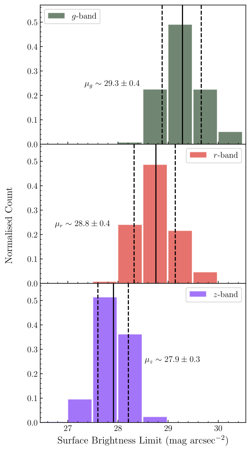
Figure 1: Histogram of the $3\sigma$ limiting surface brightness magnitudes for DECaLS images in the $g$ (top), $r$ (middle), and $z$ (bottom) bands. The median (solid line) and 68.2 per cent confidence interval (dashed lines) were estimated by determining the limit in $\sim$2,000 images. For each image, we followed the method set out in Román et al. (2020) and used randomly sampled $10\times 10$ arcsec² boxes.

DECaLS aimed to identify targets for the Dark Energy Spectroscopic Instrument (DESI) survey and used the 4m Blanco telescope at the Cerro Tololo Inter-American Observatory in Chile. Around 9000 deg² of the sky was imaged using a three-pass tiling system, where each pass was slightly offset from the others. The survey was kept as uniform as possible by using dynamic observation to automatically select targets and exposure times based on observing conditions. The result of this was around 835 million objects imaged in the g, r, and z bands with a native pixel scale of 0.262 arcsec² px^-1. The limiting point source depth in the g band is 23.95 (AB) for a median 5$\sigma$ detection. We estimated the 3$\sigma$ limiting surface brightness magnitude in $10\arcsec\times 10\arcsec$ boxes to be $\mu_{r}\sim 28.8$ mag arcsec^-2, by following the procedure set out in Román et al. (2020). Figure 1 presents normalised histograms and median estimates of the limiting surface brightness magnitudes across $\sim 2000$ images of galaxies for each DECaLS band. Our estimates of the DECaLS surface brightness limited depth are similar to those quoted in other studies (e.g. Román et al., 2021; Martínez-Delgado et al., 2021).

2.2 Galaxy Zoo DECaLS

We made use of publicly available data products produced by W22 in the form of both galaxy images and classifications. In W22, the authors used DECaLS data to construct RGB Portable Network Graphics (PNG) images of the subset of galaxies that were included in the NASA Sloan Atlas (NSA). The NSA contains a catalogue of various parameters for local galaxies imaged mostly in SDSS and GALEX. Basing the sample on the NSA introduced two selection cuts: most selected galaxies are brighter than $m_{r}=17.77$ unless they were imaged in deeper SDSS fields, and the sample has a maximum redshift of $z=0.15$. Additionally, W22 added two further cuts limiting the selection to galaxies with a Petrosian radius of at least 3 arcsec – such that the galaxies were sufficiently resolved for classification – and discarding any incomplete images where more than 20 per cent of the pixels in any band were missing. In total, the remaining sample comprised almost 314,000 galaxies.

W22 constructed their PNG images to be $424\times 424$ pixels by downloading the FITS files from the Legacy Survey Cutout service. They ensured that the whole galaxy was suitably visible on the image by resizing the image to an appropriate interpolated arcsec per pixel scale. They then multiplied the g, r, and z band fluxes by 125.0, 71.43, and 52.63, respectively, such that the false colour images had an appropriate range of colours in RGB; W22 chose these values by hand. The pixels with low fluxes were then desaturated to avoid a speckled effect in the images. Finally, the fluxes were scaled by $\sinh^{-1}(x)$ to compensate for the wide range of pixel values, linearly rescaled to be in the range $(-0.5,300)$ to remove the brightest pixels, and then clipped to the usual $(0,255)$ range for PNG files.

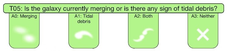
(a) Merger question for DR1&2 campaigns.

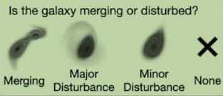
(b) Merger question for DR5 campaigns.

Figure 2: Galaxy Zoo DECaLS decision tree merger question presented to volunteers. The question was aimed to establish if galaxies were merging or disturbed in some manner and changed between the DR1&2 (2(a)) and DR5 campaigns (2(b)). Both figures were adapted from Walmsley et al. (2022, W22).

W22 used three Galaxy Zoo: DECaLS (hereinafter GZD) campaigns to obtain volunteer classifications for all galaxy images; each campaign corresponded to a different DECaLS data release – DR1, DR2, and DR5. Volunteers were asked a series of questions in a decision-tree structure to classify the bulk morphology of the galaxy, such as identifying if the galaxy was early- or late-type, how many spiral arms there were, and if a bar or bulge was present. Between DR1&2 and DR5, the decision tree questions were changed to improve clarity and direct classifications towards more specific scientific goals. For the DR1&2 campaigns, a median of 38 volunteers responded for each galaxy. However, the significantly larger DR5 campaign had a median of just five volunteers per galaxy.

As part of both decision trees, the volunteers were asked to indicate if the galaxy was merging or disturbed in some manner, the latter of which we took as a proxy for the potential to have a tidal feature. Figure 2 provides the options for indicating a disturbance presented to volunteers in both the DR1&2 (2(a)) and DR5 (2(b)) decision trees. W22 changed the possible answers for the merger question between DR1&2 and DR5 to reflect what the volunteers would see in the image more directly. In particular, major and minor disturbance labels referred to the extent and size of the debris, not necessarily the origin of the disturbance as a major or minor event. Hence, galaxies indicated as either a major or a minor disturbance were likely to have tidal features.

The classifications from the GZD campaigns were then processed and used to train a machine-learning classifier. The classifier constructed by W22 was a Bayesian Convolutional Neural Network based on the EfficientNetB0 architecture (Tan & Le, 2019). It was trained to predict how volunteers would have responded to the DR5 decision tree, and its accuracy varied from 77 to 99 per cent compared to the volunteer responses depending on the question being considered. We used the catalogue of predictions and the corresponding images as a starting point for our analysis.

2.3 Sample Selection

From the GZD data, we generated a sample of galaxies with a high likelihood of having tidal features by imposing three selection criteria in addition to the cuts introduced in W22. We first limited the sample to have an absolute magnitude in the range $-19\geq M_{r}\geq-22$. Removing the faintest galaxies restricted the number of contaminating intrinsically irregular galaxies, most of which are fainter than $M_{r}\leq-19$ in the local universe (Ann et al., 2015). At the surface brightness depth of DECaLS, faint irregular galaxies were often difficult to distinguish from tidally-disturbed galaxies. To avoid generating necessarily uncertain classification labels for them, they were removed.

The remaining two selection criteria were based on the machine-learning predictions for questions in the catalogue. Images predicted to have a greater than 0.1 chance of having an image artefact were removed. Finally, the last criterion selected the galaxies most likely to have some tidal feature, allowing us to reduce the number of galaxies to a manageable amount. Any galaxy with a prediction of greater than 0.4 in either the merging_major-disturbance_fraction (hereinafter major) or merging_minor-disturbance_fraction (hereinafter minor) columns in the catalogue was assumed to potentially include a tidal feature and was thus retained. W22 recommended using major greater than 0.6 and minor greater than 0.4 to identify post-merger and low surface brightness galaxies. We randomly sampled and inspected a small number of galaxies with varying values of both major and minor, and from this extended our threshold to include both major and minor values greater than 0.4.

Of the roughly 314,000 galaxies, 1,935 passed the above selection criteria and were assumed to be tidally disturbed. Images for seven of these were not included in the data set produced by W22, giving a set of 1,928 galaxies to visually inspect for tidal features. Furthermore, we generated a complementary sample of 1,928 galaxies assumed not to have tidal features by randomly sampling those with minor, major, and merging_merger_fraction predictions of less than 0.08. We did not visually inspect this undisturbed sample, but it was included in the training set for the convolutional neural network.

3 Initial Visual Inspection

3.1 Preparation for Inspection

We began by regenerating the thumbnails of the tidal feature sample using a more optimal stretch that enhanced the low surface brightness regions. FITS images of $500\times 500$ pixels centred on each galaxy were downloaded from the Legacy Survey cut-out service at the same interpolated pixel scale as in W22. We then stacked the images by summing the g, r, and z bands, ensuring sensitivity to tidal features regardless of their colour.

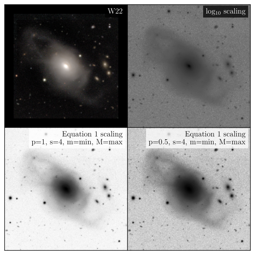
Figure 3: The galaxy J094036.39+033436.9 as an example of the images presented to the inspector during the visual inspection process. The top left shows the image produced by W22, the top right shows the logarithmically scaled image, and the bottom row shows the novel pixel scaling algorithm introduced in this work and described by Equation 1 with the parameters $M=\max({\text{pixel values}})$, $m=0$, $s=4$, and $p=1$ (left) or $p=0.5$ (right).

We tested various pixel stretch algorithms and selected the three best at enhancing the appearance of the tidal features. These were a logarithmic scaling and two novel arcsinh-based algorithms. The pixel-wise output, $x^{\prime}_{ijk}$, of the novel algorithm depended on the input pixel value $x_{ijk}$ and four other controllable parameters: the maximum $M$, minimum $m$, stretch $s$, and power $p$. The output was then

$$x^{\prime}_{ijk}=\begin{cases}0&x_{ijk}<m\\ \frac{\sinh^{-1}\left[\alpha(x_{ijk};\;s,m,p)\right]}{\sinh^{-1}\left[\alpha(M;\;s,m,p)\right]}&m\leq x_{ijk}\leq M\\ 1&x_{ijk}>M\end{cases}\\$$ (1a)

where

$$\alpha(x;s,m,p)=\left(\frac{s|x-m|}{1+s|x-m|}\right)^{p}$$ (1b)

and was inherently constrained to be in the range $\left[0,1\right]$ due to the normalisation. During the visual inspection, we presented the inspector with these three scaled images alongside the original produced by W22. An example of the images presented during the visual inspection is provided in Figure 3.

3.2 Inspection Process

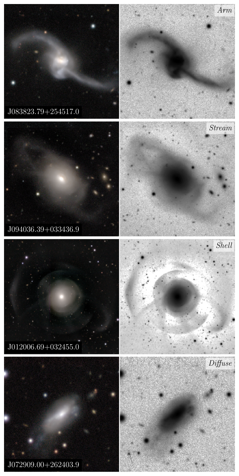
Figure 4: Examples of each of the four categories of tidal features that we visually searched for in the DECaLS sample: arm, stream, shell, and diffuse. Each inspector would identify which features were present on the image, selecting all that were visible. Left-hand images were created by W22 and were used to train the network described in Section 4.1, right-hand images show the same galaxy using the Equation 1 pixel scaling.

We used the Zooniverse.org platform to make and record classifications for each of the 1,928 galaxies likely to show tidal features. Zooniverse has become a valuable tool for detection and classification studies, most notably including citizen scientists (Lintott et al., 2008) such as the volunteers in W22. In our case, each of the inspectors (the authors) was presented with the four associated images for each galaxy, as described above and shown in Figure 3. The inspector was then asked to classify the galaxy into five non-exclusive categories: arm, stream, shell, diffuse, or uncertain. Where there were multiple features of different kinds, the inspector selected all that applied, and where there were several of the same features, the appropriate category was selected only once. Each of the three inspectors provided separate classifications, which were then combined to produce a label for every galaxy.

The choice of these categories was motivated in part to follow similar works in the literature and to have some connection to the potential astrophysical origin of the feature, thus allowing the classification to be driven towards specific science cases. Figure 4 provides an example of each type of tidal feature we chose, and a brief description of their characteristics is provided below:

Arm: arms form from material that originates in the host galaxy, so the surface brightness of these features is generally higher close to the galaxy’s main body and tails off with increasing radial distance. They have colours similar to the host galaxy and should be clearly connected to it. We follow the nomenclature of Atkinson et al. (2013) and call these features arms but note that they are also referred to as tails in the literature (see e.g. Bílek et al., 2020; Martin et al., 2020; Sola et al., 2022; Desmons et al., 2023a).

Stream: streams have similar morphologies to arm features; however, they are not connected to the parent galaxy. They are often brightest near the remaining core of the progenitor, with surface brightness falling off as one moves away from this. They are usually far fainter than the parent galaxy. These features could be short, linear, or wrapped around the parent galaxy, depending on the type and inclination of the orbit. Most other literature works include a stream class (Kado-Fong et al., 2018; Bílek et al., 2020; Martin et al., 2020; Sola et al., 2022; Desmons et al., 2023a) and we note that this class contains the linear class from Atkinson et al. (2013).

Shell: shells generally have some symmetry to the shape, such as a shell or fan-like body around the host galaxy and have well-defined, often brighter, edges or caustics. We combine the shell and fan classes from Atkinson et al. (2013), and similarly to streams, the same literature works include a shell class.

Diffuse: diffuse features lack any well-defined symmetry to the feature or do not fit well into any of the other categories. They have reasonably irregular or asymmetric shapes; however, there can be some ambiguity between genuinely low surface brightness irregular galaxies and diffuse debris. A critical diagnostic is the contrast between the galaxy’s central region and the debris. When this is small, the systems are likely to be genuinely low surface brightness or irregular galaxies, whereas significant contrast is probably more reflective of debris. The diffuse class is similar to those from Atkinson et al. (2013), Martin et al. (2020), and Desmons et al. (2023a) with the same name.

Uncertain: when a galaxy could not be reliably classified into one of the above categories, it was labelled uncertain. Most of these galaxies consisted of those too faint or small to reliably say any feature was present or those insufficiently distinct from intrinsically irregular galaxies.

We chose not to include some classes from other works such as bridges, merger remnants, or double nuclei (Martin et al., 2020; Desmons et al., 2023a) as our focus concentrates on post-merger features, and these classes likely represent a mid-merger phase.

3.3 Classification Demographics

We combined the inspector classifications for every galaxy by considering where the majority (at least 2 out of 3) agreed that a particular feature was present. For example, if one inspector said arm + stream, another said arm, and the last indicated stream + shell, the resulting label would be arm + stream. We follow this process for uncertain labels, but where a galaxy was given an uncertain designation, it was not given any other label regardless of whether it would have received a label corresponding to a tidal feature. Where the individual classifications did not agree on any label, the galaxy was classified as none. Thus, we end up with seventeen possible labels based on the various combinations of features. Those being none; uncertain; arm; stream; shell; diffuse; arm and stream; arm and shell; arm and diffuse; stream and shell; stream and diffuse; shell and diffuse; arm, stream and shell; arm, stream and diffuse; arm, shell and diffuse; stream, shell and diffuse; and arm, stream, shell and diffuse.

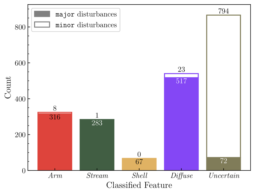
(a) Categories of tidal features.

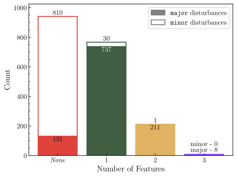
(b) Number of tidal features.

Figure 5: Demographics of the visual inspection of galaxies for the presence of tidal features. Each galaxy was labelled by considering where two out of three inspectors agreed a given feature was present. (5(a)) provides the number of galaxies that have arm, stream, shell, diffuse, and uncertain labels. Galaxies labelled with multiple features are counted multiple times in this Figure. (5(b)) indicates how many galaxies contained multiple features. Galaxies where no label was agreed on or labelled as uncertain are included here as none. In both (5(a)) and (5(b)), the histograms are split by whether the W22 classifier rater the galaxy highly in the merging minor-disturbance fraction or merging major-disturbance fraction columns. Finally, (5(c)) shows the overlap between the classifications made. In all three, the numbers shown indicate the number of galaxies in that category.

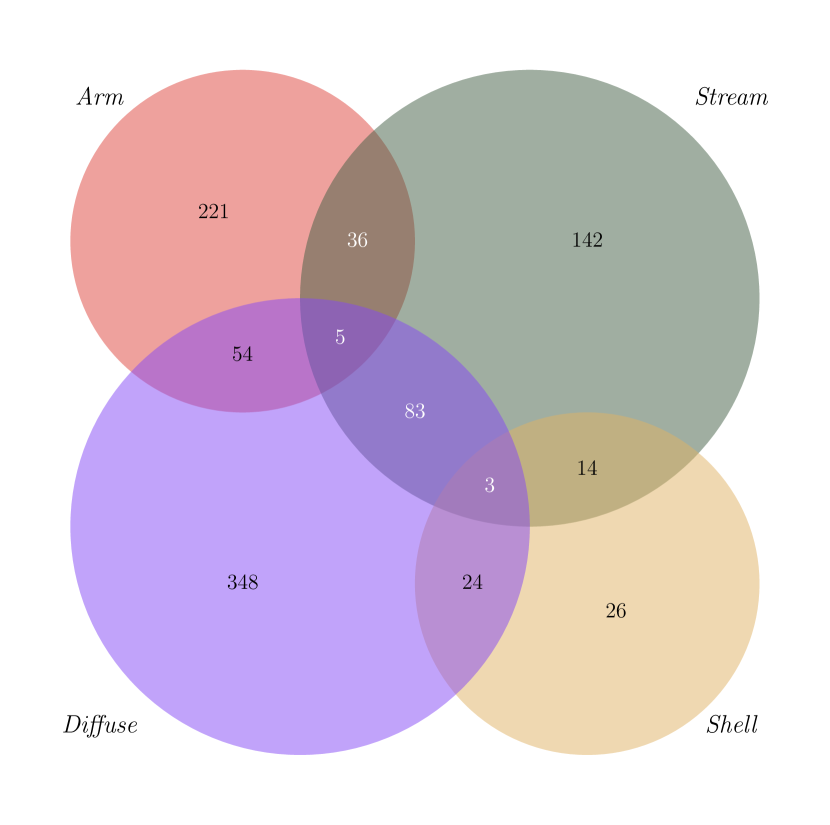
(c) Overlap in classifications of feature categories.

Figure 5: continued

Demographics of the visual inspection of galaxies for the presence of tidal features. Each galaxy was labelled by considering where two out of three inspectors agreed a given feature was present. (5(a)) provides the number of galaxies that have arm, stream, shell, diffuse, and uncertain labels. Galaxies labelled with multiple features are counted multiple times in this Figure. (5(b)) indicates how many galaxies contained multiple features. Galaxies where no label was agreed on or labelled as uncertain are included here as none. In both (5(a)) and (5(b)), the histograms are split by whether the W22 classifier rater the galaxy highly in the merging minor-disturbance fraction or merging major-disturbance fraction columns. Finally, (5(c)) shows the overlap between the classifications made. In all three, the numbers shown indicate the number of galaxies in that category.

While the ultimate goal of the visual inspection was to generate labels to train a CNN, it is also of some interest to explore the properties of the classifications. Hence, in Figure 5, we present the demographics of our classifications, split based on whether the prediction of the galaxy was from the major (solid) or minor (outline with a hollow centre) columns in W22. In both (5(a)) and (5(b)), the numbers provided represent the number of galaxies in each category, again divided based on the W22 prediction.

Figure 5(5(a)) provides the number of galaxies with each feature class, noting that this figure will count galaxies with more than one feature multiple times. Both stream and arm features appear to be roughly as common as each other (16.8 and 14.7 per cent of the inspected galaxies, respectively), diffuse features appear to be the most common (28.0 per cent), and shells the least (only 3.5 per cent).

Figure 5(5(b)) shows the number of features present for each galaxy; uncertain galaxies have been included in the none category as there was no useable feature present. Most galaxies exhibit a single tidal feature at the surface brightness depth of DECaLS. For some galaxies, all the authors agreed that there was a feature (i.e. not labelled uncertain), but no consensus on the type was reached. Hence, more galaxies show no feature than those labelled uncertain. Figure 5(5(c)) provides the Venn diagram of the classification demographics. We observe that no galaxy contains all four features, and no combination includes both an arm and a shell feature.

What is of particular note is the minor galaxies. As shown in Figure 5, most of the uncertain and none feature categories are occupied by those indicated as minor in W22. Of the 841 galaxies labelled by W22 as a minor disturbance (43.6 per cent of the inspected sample), less than 4 per cent had a label that was not uncertain. We, therefore, decided to entirely remove all minor galaxies and instead create our training sample from the major disturbance galaxies only. To maintain a roughly balanced weighting between the disturbed and undisturbed samples, we removed an equal number of undisturbed galaxies from the complementary set, reducing it to 1,087.

We believe this discrepancy between the predictions from the W22 classifier and our inspection results from a mixture of effects. In most cases, the volunteers rated the galaxy as highly likely to have a minor disturbance and the automated classifier followed these labels. However, in some cases, the automated classifier overestimated the fraction of votes for the minor disturbance such that it was above our threshold even though the volunteers had rated it unlikely. As a curiosity, we also note that a significant proportion ($\sim$20 per cent) of the minor galaxies we remove received fewer than five votes from the volunteers. In addition to removing all of the minor galaxies, we excluded those that received an uncertain or none label. Thus, our final training sample included 956 galaxies with tidal features (about one-half of the 1,928 we initially classified) and 1,087 without.

4 Automated Classification

In total, the visual inspection process took $\sim 77$ hours for just 1,928 galaxies. This was in part due to the need to identify faint and subtle structures, which may have increased the inspection time compared to other inspection problems (e.g., spiral vs. elliptical). Regardless, this was a significant amount of effort on a relatively small data set, especially compared to the volume of data expected from forthcoming surveys. Therefore, we used our set of visually inspected galaxies to provide a training set to develop an automated process for classifying tidal features with the intention of applying the process to future data later.

4.1 Architecture

In essence, a CNN is a model comprising a series of different computations or operations and how these are organised is known as the architecture. The architecture can be considered a series of connected nodes grouped into layers. All the nodes in a layer perform the same operation, each representing where a given operation occurs. The outputs from previous nodes are used as inputs to the next layer of nodes. In a typical CNN used for classification, the layers can be grouped into two parts: a feature extraction part and a classification part. The feature extraction part aims to generate a suitable representation of the image and any features where similar images cluster together in a multi-dimensional space, known as the latent space (e.g. Alzubaidi et al., 2021). The network’s classification part takes the latent space representation of the image and applies a series of linear combinations with weights and biases to generate a prediction. Overall, the goal is for the network to optimise its parameters such that the output matches the target for the given task as well as possible.

Table 1: The architecture of the convolutional neural network. The architecture sets out the sequential (top to bottom) order of the layers of different operations, the number of nodes in each layer, the activation functions used, and the number of trainable parameters in that layer. Bracketed numbers show the number of nodes or parameters for the case of the binary network (see Section 5.2.1). See text for details of the operations performed in each layer.

Layer	Nodes	Kernel Size	Activation	Parameters
Conv2D	32	$3\times 3$	ReLU	896
MaxPool2D	–	$2\times 2$	–	–
Conv2D	48	$3\times 3$	ReLU	13,872
MaxPool2D	–	$2\times 2$	–	–
Conv2D	64	$3\times 3$	ReLU	27,712
MaxPool2D	–	$2\times 2$	–	–
Flatten	–	–	–	–
Dense	64	–	ReLU	3,686,464
Dropout (0.5)	–	–	–	–
Dense	4 (or 1)	–	Sigmoid	260 (or 65)
Total parameters			3,729,204 (or …,009)

We used a modified version of the network architecture used by W19 and subsequently adopted by DS23. The architecture is provided in Table 1, along with the number of trainable parameters associated with that layer, and is described in more detail below. Our aim for this work was not to provide a definitive solution to this problem but rather to demonstrate that it was possible to use CNNs to classify different kinds of tidal features, so we did not further optimise the hyperparameters of the network beyond that of W19. Instead, we focused on testing the applicability of the already optimised network to our slightly different task.

The extraction part of the network was composed of three convolutional blocks: a 2D convolution layer with a $3\times 3$ kernel, a Rectified Linear Unit (ReLU) activation function, and a $2\times 2$ shaped max pooling. The blocks consisted of 32, 48, and 64 nodes, respectively. The convolutional layer works by convolving each channel of the input image (e.g. survey bands) with a kernel. The resulting outputs are then summed over the number of input channels. This process is repeated for all m nodes of the convolutional layer. The network often comprises a series of convolutional layers that apply this process to transform the m nodes of the previous layer to the n of the next (e.g. Goodfellow et al., 2016). Pooling layers reduce the size and training time of the network by replacing values over a specified region with a summary value, such as the maximum or average (e.g. Alzubaidi et al., 2021). This also induces the network to be invariant to small translations in the input image (e.g. Goodfellow et al., 2016).

The classification part consisted of two fully-connected (or dense) linear layers of 64 nodes and the appropriate number of output nodes depending on the task, with dropout applied between these layers. Each node in the fully-connected layer applies a linear combination of weights and biases to all of the outputs from the previous layer (e.g. Goodfellow et al., 2016).

During training, a portion of the data is reserved for validation; this validation data effectively serves as unseen data to test the generalisation of the network. When the metrics used to monitor training performance begin to diverge from those evaluated on the validation data, this can indicate that the network is overfitting the training data. We employed both dropout – between the fully-connected layers – and early stopping to prevent the network from overfitting to the training data, which would negatively impact the generalisation of the network to unseen (or testing) data. Dropout randomly removes neurons at each step during training with a specified rate (Srivastava et al., 2014), which we chose to be 50 per cent in line with W19. This prevented particular parts of the network from being overly crucial for a given classification and meant the network had to learn many independent features (Alzubaidi et al., 2021). Early stopping monitors the validation loss metric. It determines whether an improvement has been made based on the minimum value of the loss and the loss from the current epoch. After a specified number of epochs – the patience period – with no improvement, the network stops training and restores the network parameters that obtained the best value of the validation loss. We chose this patience period to be 40 epochs.

4.2 Augmentation

We can see from Table 1 that there were $\sim 10^{6}$ parameters that needed to be constrained through training. This meant we required a large and diverse training set to avoid overfitting the data. Unfortunately, we could not expand our training set beyond the galaxies we had already inspected for tidal features. However, data augmentation allowed us to artificially expand the training set (see, e.g. Goodfellow et al., 2016; Shorten & Khoshgoftaar, 2019; Alzubaidi et al., 2021) without visually classifying further galaxies. The presence or absence of a feature was independent of transformations or augmentations of the input image, such that instances of the same image can be used repeatedly during training. W19 took this approach when they were training their network on the 305 galaxies inspected by Atkinson et al. (2013). We applied the following augmentations to the data randomly, noting a slight modification from W19 in the rotation augmentation:

1. horizontal or vertical flip or both

2. rotation in the range $\left[-\frac{\pi}{2},+\frac{\pi}{2}\right]$

3. translation up to $\pm$5 per cent along both axes

4. zoom in or out up to 10 per cent

After these augmentations, we downsized by rebinning the images to $256\times 256$ pixels. We found that resizing the images improved the network performance on the order of a few per cent and chose $256\times 256$ as the optimal.

4.3 Multi-Label Results

As with the other works on the subject (e.g. ; ; ), we employ the true positive rate (TPR), false positive rate (FPR), and area under the curve (AUC) metrics to measure the performance of our classifier. Each metric compares some combination of the number of true positives, true negatives, false positives, and false negatives, abbreviated as TP, TN, FP, and FN, respectively. The predictions from the network were separated into positive and negative based on some predictive threshold $P$, and a binary label was assigned for each class based on whether the prediction was greater or lesser than the threshold. These were then compared to labels assigned during the visual inspection to determine whether the predictions were true or false. The FPR

$$\text{FPR}=\frac{\text{FP}}{\text{FP}+\text{TN}}$$ (2)

is a measure of the amount of contamination in the predicted positive samples or the probability a predicted positive example is negative. Conversely, the TPR

$$\text{TPR}=\frac{\text{TP}}{\text{TP}+\text{FN}}$$ (3)

provides the probability that positive examples will be predicted as positive, or equivalent, the fraction predicted during testing. The AUC score measures the area underneath the curve created by the FPR and TPR values

$$\text{AUC}=\int^{1}_{0}\text{TPR}\left(\text{FPR}\right)\text{d}\text{FPR}$$ (4)

for each value of $P$. An AUC of 0 means that the predictions were completely wrong, whereas an AUC of 1 means that the predictions were entirely correct.

We used our training set of 2,043 galaxies (discussed in Section 3) to train trials of the network. For each trial, 20 per cent of the data were randomly selected as unseen data to test the network’s performance. The remaining data was split 9:1 for training and validation, respectively. At each step in training, the images were loaded in and randomly augmented. We applied a weighting

$$w_{i}=\frac{n_{\text{samples}}}{n_{\text{classes}}n_{i}}$$ (5)

to the training for each class to compensate for the imbalance between the different classes. The weighting was based on the total number of training samples in the set, $n_{\text{samples}}$, divided by the product of the number of classes, $n_{\text{classes}}$, and the number of examples for that class, $n_{i}$. This prioritised training on the higher weighted classes to compensate for the fewer numbers.

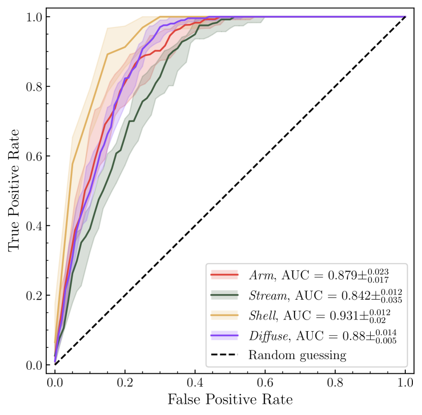
(a) ROC curves for each class

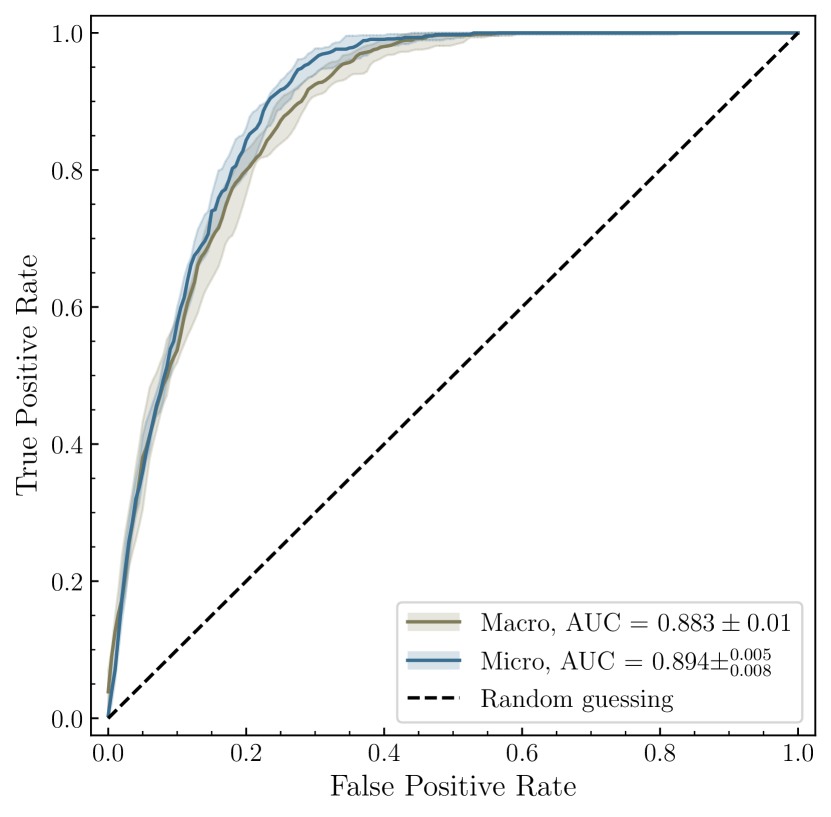
(b) Averaged ROC curves micro (label-wise) and macro (class-wise)

Figure 6: Median Receiver Operating Characteristic (ROC) curves for each of the categories of tidal features (6(a)) and the micro- and macro-averages (6(b)). The median is calculated by averaging over ten independent trial runs of the network, and the shaded regions indicate the 68.2 per cent confidence interval. The ROC curve indicates how the fraction of correctly identified galaxies (true positive rate) and the fraction of incorrectly identified galaxies (false positive rate) change with respect to the predictive threshold – that being the value above which the output of the classifier would be taken to indicate a prediction the feature was present. The macro-average averages each of the classes’ ROC curves, and the micro-average treats each label independently.

Figure 6 shows the median receiver operating characteristic (ROC) curve for ten trial runs of the network with the shaded region showing $\pm 1\sigma$. The ROC curve shows the relationship between FPR ($x$-axis) and TPR ($y$-axis) for different predictive thresholds, where lower thresholds result in more completeness but also more contamination. As mentioned, each trial network was trained for between 40 and 300 epochs, with the median number of epochs being $204.5_{-58.4}^{+63.7}$. It is expected that random guessing would yield an equal TPR and FPR across all thresholds, and hence we hope and do indeed observe in Figure 6 that the ROC curve is well separated from the random guessing line. Figure 6(6(a)) shows the ROC curve for each class – where each class is treated independently – and (6(b)) provides the micro- and macro-averages. The macro-average averages over each of the classes’ ROC curves with an equal weighting, and the micro-average determines the ROC curve, considering each label as independent. As the diffuse class is the most populous, it makes sense that the micro-average (which weights each galaxy equally) should coincide closely with this.

Table 2: Median true positive rates and 68.2 per cent confidence intervals for a fiducial false positive rate of 0.2 for each category of tidal feature and the micro- and macro-averages. The median is determined by averaging over ten trial runs of the network.

Feature	Median	$+1\sigma$	$-1\sigma$
Arm	0.811	0.058	0.065
Stream	0.657	0.050	0.084
Shell	0.913	0.060	0.059
Diffuse	0.823	0.014	0.079
Micro-average	0.844	0.018	0.049
Macro-average	0.802	0.027	0.047

Although the performance is very encouraging across all classes, some variations can be seen. In particular, Stream features were recovered at a lower rate than other classes, with the network obtaining a median TPR of $0.657^{+0.050}_{-0.084}$ for a fiducial contamination of 20 per cent (i.e. at an FPR of 0.2). In contrast, shell features were recovered well with a median TPR of $0.913^{+0.060}_{-0.059}$ for the same degree of contamination. Table 2 provides the median TPR values for each class and the micro- and macro-averages at the reference 20 per cent contamination.

5 Discussion

Our results are the first demonstration of using deep learning to classify different types of tidal features. This presents an excellent opportunity for forthcoming imaging surveys such as LSST (Ivezić et al., 2019) and Euclid (Laureijs et al., 2011) to investigate the occurrences of the different species of tidal feature and thus, hopefully, shed light on the formation mechanisms and provide substantial data for population studies. As our primary focus for this work was to demonstrate the application of CNNs to classifying different categories of tidal features, we leave investigations of the properties and populations of these features to subsequent works. Although we observed a good performance for our network, we do note that there are imperfections, some of which are discussed below. In particular, we observed that the output predictions from the network do not always necessarily reach a value of 1 (i.e. the label value for present). If this output is thought to be a probability that a feature is present, then the network is not confident that a feature is there. However, it is always possible to select some value of the predictive threshold to separate positive and negative predictions between the minimum and maximum output from the network. Thus, the performances seen in the ROC curves remain unchanged by reducing the range of predictive thresholds.

5.1 Variations in class performance

It is evident from Figure 6(6(a)) and from Table 2 that the network was best performing at recovering shell features. We suspect this may be due to the characteristic hard edges or caustics in shells, which the network might find relatively easy to detect. Additionally, applying the class weighting during training should counter the effects of the class imbalance, and shells would have received a significantly higher weighting than the other classes as there were only 67 galaxies in the sample with shell features.

Furthermore, we suspect that the arm and stream classes are the least well-performing due to the similarities between the classes. We often found it difficult during the visual inspection process to separate instances of the two classes as the defining features of the classes are very similar, often with the inspector having to make some estimation of the likely origin of the feature. In particular, we note that inspectors frequently disagreed on whether a feature was a stream or arm. This suggests that these classes could be combined or the visual inspection process improved to ensure a clearer distinction between the classes, such as more explicit instructions on the differences. We suspect, then, that the network is susceptible to this uncertainty in the actual label of the feature and similarly struggles to separate the two similar classes. We investigate later the impact of improving the classification scheme to reduce label noise (Section 5.4).

5.2 Comparison to the Literature

In this Section, we compare our results to those from the literature. First, we default back to comparing a binary classification to match the work already undertaken. We then compare our multi-label results to the binary classifications of the literature. Finally, we identify whether streams in the DECaLS area identified by Martínez-Delgado et al. (2023) were identified by our network.

5.2.1 Binary Results

To begin the comparison of our work to that of W19, DS23, and DBL23, we performed a binary classification. That is, where we cared only to identify if a tidal feature was present on the image rather than what that tidal feature was. We constructed a binary training set by taking those galaxies where the majority of inspectors had identified some tidal feature in the visual inspection process, including those where no consensus was reached as to the exact category of the feature. The resulting binary training set consisted of 1,062 galaxies with a tidal feature and a complementary set of 1,087 galaxies without a feature, the same galaxies used previously.

As before, we preprocess the data by applying random augmentations and resizing the images to be $256\times 256$. We trained ten different trial runs of the network for a maximum of 300 and a minimum of 40 epochs. Twenty per cent of the training set was reserved as entirely unseen for testing, and the rest was split between training and validation. We evaluated the network’s performance using the testing set. Similarly, where before we weighted the training to compensate for the imbalance between the categories of tidal features, we now applied a weighting to the tidal and non-tidal categories. This weighting was used such that the network was not trained to be biased towards the more populous class.

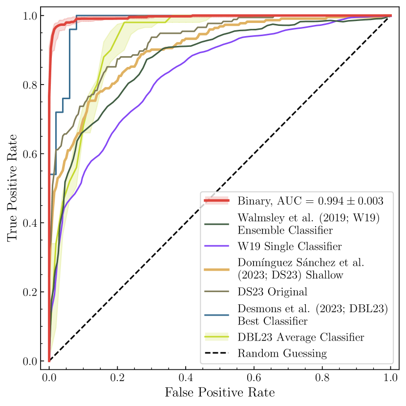
Figure 7: Median ROC curve for the binary classification with comparative literature results. The binary classification considers only positive and negative incidences of any tidal feature, unlike the multi-label classification, which aims to identify the type of tidal feature. Shaded regions indicate the 68.2 per cent confidence interval; again, the median is determined over ten network trials. We include both the single and best-performing ensemble classifiers from W19, both shallow and original samples from DS23, and the best-performing classifier and our determination of the median of other classifiers from DBL23.

Figure 7 shows the median ROC curve for the binary classification; again, the shaded area shows the 68.2 per cent confidence interval. It is evident from the Figure that our classifier has an outstanding performance, reaching an AUC score of $99.4\pm 0.3$ per cent. ROC curves from W19, DS23, and DBL23 are also shown in the Figure.

However, we note that our binary sample is likely to be a highly idealised scenario. The sample has already been split according to a binary classification schema during the sample selection process, where we selected only galaxies where the W22 classifier indicated that there may be a potential tidal feature. Thus, we expect images where the network may struggle to predict whether a tidal feature is present to have been excluded from the binary classification set. Therefore, the performance on unbiased data is likely to be worse than this. Our multi-label set represents a new classification schema, so we expect this problem to be a lesser issue as those images have not necessarily been selected as good or bad at identifying categories of tidal features.

5.2.2 Multi-Label Comparison

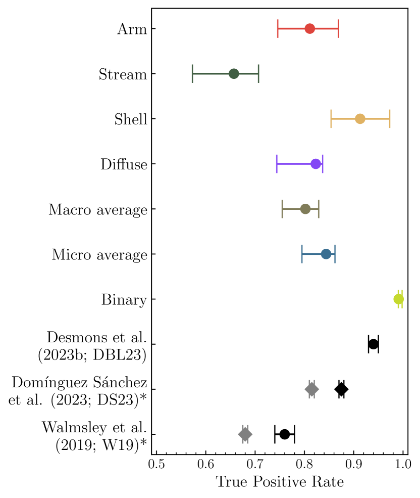
Figure 8: Median true positive rates (TPR) at a specified false postive rate of 0.2 for each class, micro- and macro-average, and a binary classification identifying any tidal feature. The median is calculated by averaging over ten trial runs of the network, and the error bar represents the 68.2 per cent confidence interval. Additionally shown are corresponding values from the binary classifiers of DBL23, DS23 for both the network trained with (grey) and without (black) shallower data, and W19 for both a single CNN (grey) and the average of two ensembles of CNNs (black). See text for details. *Diamond markers show points where the error comes from plot estimation error; the respective authors report all others.

Figure 8 presents the median TPR values for each category of tidal feature, the macro- and micro-averages, and the binary classification (from Section 5.2.1) for an FPR of 0.2, as well as the equivalent for W19, DS23, and DBL23. All values are included with an associated error either reported by the relevant authors, shown as circle markers, or estimated by us in the reading of appropriate plots, which are provided as diamond markers.

We see in Figure 8 that the performance of our networks at identifying the arm and diffuse classes are comparable to both the ensemble classifiers of W19 and to the shallow training sample of DS23, the micro- and macro-averages are similarly comparable to those works. We further note that we can obtain performances similar to that of DBL23 for our shell class using our supervised approach, which is perhaps surprising given that the shell class only has a few training examples. Finally, although not as good as the other classes, the stream class is approximately on par with the single classifier from W19. It may be possible then to improve the performance of the stream class by using an ensemble of classifiers similar to the work of W19 for binary tidal feature detection.

It is important to recall, however, that detections of tidal features depend heavily on the limiting surface brightness magnitude of the survey (e.g. Johnston et al., 2008; Vera-Casanova et al., 2022). Thus, we expect that the tidal features are more clearly visible in deeper data, and as such, comparing network performances on varying depth data should take this into account, with our expectation being that networks trained using deeper data will have better performance. We do somewhat observe this trend for the three works we have compared to when considering the limiting surface brightness ($\mu_{r}\sim 28.8$ this work; $\mu_{r}\sim 27.1$ W19; $\mu_{r}=26-35$ DS23; $\mu_{r}\sim 29.82$ DBL23; in mag arcsec^-2 ). We believe this may also be the case for class-wise performances with the brightest features, the bright edges of the shell features, performing better than the slightly fainter diffuse and arm features, which perform better than the faintest stream features. Overall, we conclude that our work is consistent with the literature and that, given a suitably large training set, detecting different types of tidal features is possible.

5.2.3 Stellar Stream Legacy Survey

Martínez-Delgado et al. (2023) introduced the Stellar Stream Legacy Survey to identify stellar streams in the local universe. They use data from the DESI Legacy Imaging Survey DR8, which includes DECaLS, as well as the Beijing-Arizona Sky Survey and Mayall z-band Legacy Survey (BASS and MzLS, respectively; Dey et al., 2019). They re-reduced the raw Legacy Surveys data using a bespoke sky subtraction algorithm (see Martínez-Delgado et al., 2023, for details) and then visually inspected a sample of 689 galaxies. From this, they selected 24 galaxies with stellar streams – explicitly chosen to cover a range of morphologies, surface brightnesses, and distances – and used noisechisel (Akhlaghi & Ichikawa, 2015) to confirm the detections.

We investigated the overlap between the 24 galaxies with stellar streams they identified and our sample. Of the 24 galaxies in their sample, we find only 18 of these were imaged in DECaLS DR5. Furthermore, 4 of these galaxies were not imaged with SDSS and, as such, were excluded from our sample due to the W22 selection criteria. None of the 14 remaining streams identified by Martínez-Delgado et al. (2023) were included in the galaxies we visually inspected. Again, this stems from the W22 analysis, which yielded a major disturbance prediction from the GZD automated classifier that was somewhere between 0.08 and 0.4, and hence below our selection threshold for visual inspection. The reasons for this could either be a result of the volunteers being uncertain if the galaxy was disturbed or not or due to the inaccuracies in the classifier. Although none of these 14 galaxies were inspected by us, they had high enough prediction scores to be excluded from our assumed undisturbed sample.

In lieu of our own visual inspection of these systems, we could at least use our network to generate predictions for each of these galaxies to discover if our classifier agrees that they are tidally disturbed. Encouragingly, all 14 galaxies were identified by our network to be disturbed in some manner. This is quite a remarkable success given that our network operates on the standard imaging pipeline output without any advanced or bespoke processing to enhance the appearance of low surface brightness features beyond the work of W22. That said, at the surface brightness depth of the standard pipeline-processed DECaLS data, the tidal features were very faint. As such, the specific classification of tidal features was slightly ambiguous. Regardless, the ability of our network to confidently recover all of the Martínez-Delgado et al. (2023) streams as tidally disturbed without the need for advanced image processing is seen as very promising.

5.3 Grad-CAM Analysis

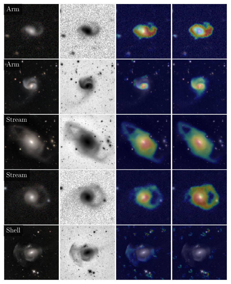
Figure 9: Outputs of a gradient-weighted class activation mapping (Grad-CAM) analysis. The analysis generated a heat map indicating where on the image the network considered important for making a particular classification (blue least to yellow/red most important). The classification being considered is written in text on each row. The left-most column shows the image of the galaxy produced by W22, and the second from the left shows the image with the low surface brightness regions highlighted according to the novel algorithm (Equation 1). The two right-hand columns show the output of the Grad-CAM analysis for the two selected best-performing models: the model that reached the lowest validation loss during training and that with the greatest testing AUC score.

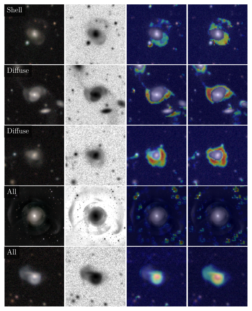
Figure 10: continued

Outputs of a gradient-weighted class activation mapping (Grad-CAM) analysis. The analysis generated a heat map indicating where on the image the network considered important for making a particular classification (blue least to yellow/red most important). The classification being considered is written in text on each row. The left-most column shows the image of the galaxy produced by W22, and the second from the left shows the image with the low surface brightness regions highlighted according to the novel algorithm (Equation 1). The two right-hand columns show the output of the Grad-CAM analysis for the two selected best-performing models: the model that reached the lowest validation loss during training and that with the greatest testing AUC score.

CNNs are prone to suffering from shortcut learning, where they can learn spurious connections between parts of the data and the desired output (see, e.g. Geirhos et al., 2020). This problem is an important issue, particularly for the generalisation of the network to unseen data, and verifying that this has not impacted the network should be a crucial part of any model development process. It is, therefore, vital to establish whether or not the network does indeed use the correct information to produce a prediction. In the context of this work, we must verify that for a given image, the network uses the galaxy and surrounding tidal features to adopt the prediction for that class.

We verified that the network was classifying the images as intended by performing a Gradient-weighted Class Activation Mapping (Grad-CAM; Selvaraju et al., 2017) analysis. In general, the analysis determines the gradient of a class score with respect to the feature map (the latent space representation) in the final convolutional layer. Then, it averages over this to assign an importance value to a particular neuron. The final heat map showing the regions of importance is generated by taking a linear combination of the importance values.

We selected the two best-performing models to analyse: the model with the lowest final validation loss and the model with the highest AUC score. Figure 9 provides some examples of the original images of the galaxies (left-most column) and a version of the image scaled using Equation 1 (middle-left) alongside the Grad-CAM heatmaps for the two models tested (two right-hand columns). Red regions on the heatmap indicate areas of high importance, yellow and green lesser, and blue with little importance.

Figure 9 demonstrates that the model identified the disturbed regions in the manner intended but shows an interesting effect where there appear to be regions of importance around background stars and galaxies. This effect can be attributed to the outer areas appearing fuzzy and faint due to limited resolution and seeing, thus resembling a diffuse feature. This effect highlights slight imperfections in how the network reaches predictions. It may be possible to counter this effect by masking background sources. Still, we emphasise the need to strike a balance between masking unimportant background sources and maintaining the faint structure of the feature. Overall, then, the network appears to be identifying tidal features in the same manner that an expert would.

5.4 Improving Classification

During the visual inspection process, reaching a complete consensus on the type of tidal feature was often challenging due to different interpretations of the instructions and characteristics that defined each feature or due to inconsistencies in individual inspectors. We also found considerable noise when considering the classifications for a particular galaxy; all three authors only agreed on every feature in 145 galaxies. As the network was trained to recreate our labels, which we only assumed to be the ground truth, we thus hypothesise that if our classifications can be improved and the noise reduced, the network performance may improve. To that end, we investigated the impact of re-classifying some galaxies with more precise instructions and enhanced images on the consensus between authors and how this, in turn, impacted CNN performance.

5.4.1 Reinspection

We improved the classification process by updating and clarifying the instructions in our decision tree. We included an initial question asking if any feature was present; if the inspector answered yes, they were then asked to identify what features. The choice of features was the same as the original inspection, however we clarified the characteristics of each feature and allowed the inspector to select whether they were confident or less confident the feature was present.

We randomly selected 50 galaxies from our training sample to test the new classification decision tree. As before, each galaxy was given a label based on the responses from the three authors. Of the 50 galaxies, 36 per cent had no change to their label, 44 per cent had a minor change, 12 per cent had a significant change, and 4 per cent had a critical change where the label was completely different from the original.

We found that the reclassification led to no overall improvement in the agreement between the authors with an equal number of labels with the same or fewer votes as the number with more votes. However, we found an impact on the confidence in the label, mainly through the addition of a less confident option. We based the confidence of the new label on the confidence options provided by the decision tree and the old confidence in part on the agreement between the authors and the selection of uncertain. Fewer labels increased in confidence than suffered a drop in confidence.

5.4.2 Retraining

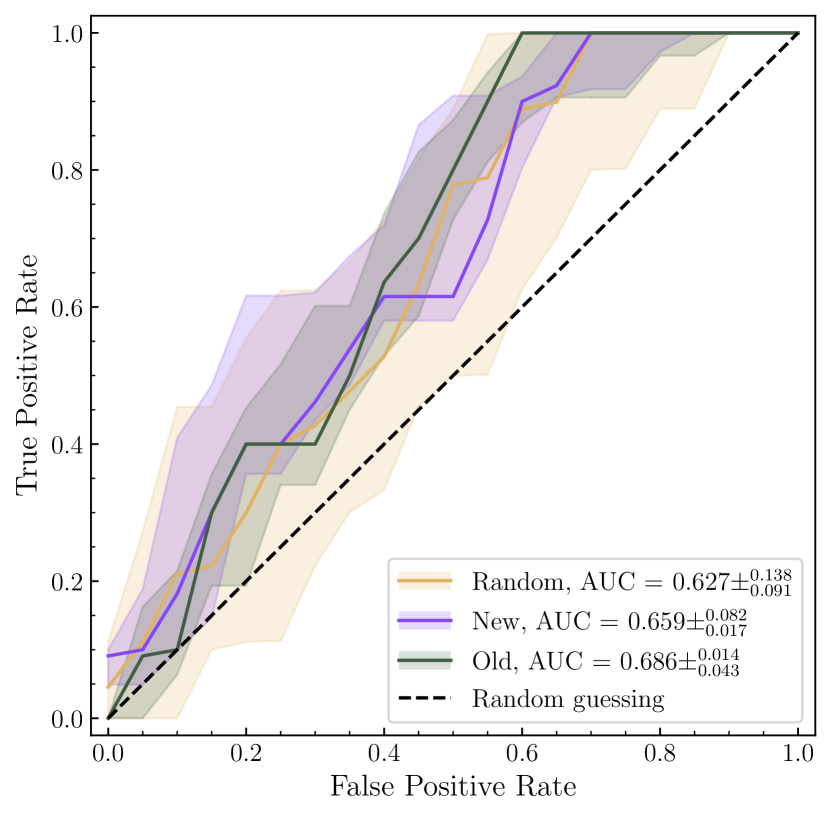
Figure 11: ROC curves from retraining the classifier on the new classifications. Each of the models in this plot was trained using $\sim$30 galaxies with the rest left for testing, the same ratios as when the classifier was trained using the full sample. The green curve provides the median of 5 trial runs of training the classifier on the original classifications of the reclassified galaxies, and the blue provides the same using the new classifications. Finally, the yellow curve is the median of classifiers trained using 20 randomly sampled sets of the full original classifications of galaxies to serve as a baseline for improved performance. Shaded regions provide the 68.2 per cent confidence interval.

We tested the impact those reclassifications had on the performance of the CNN. For the original and new classifications of the 50 galaxies, we trained five trial runs of the network and compared the median ROC curves for these two sets. As this is such a small number of galaxies, we expect the performance to be relatively poor, so we also randomly sampled 20 groups of 50 galaxies to have a baseline comparison to the network performance at that level. Figure 11 shows the median ROC curves for the original classifications, the new classifications, and the random sampling with the respective 68.2 per cent confidence interval shaded. We see evidence of a marginal improvement in the ROC curve based on moving from the original classifications to the new classifications. However, there is no improvement from the randomly sampled baseline.

We suggest that other strategies, such as masking background sources, further hyper-parameter optimisation, deeper data, or transfer learning pre-trained networks, may be better suited to improving the performance of the network. Given the satisfactory performance of the network trained on the entire sample of original classifications (Section 4.3) and the time commitment to reclassifying all 956 galaxies, we decided not to continue with reclassifying all of the galaxies.

6 Conclusions

Tidal features are a crucial probe of the hierarchical formation of galaxies, and these features contain a wealth of information that could advance our understanding of galaxy evolution. Forthcoming wide-field surveys, such as LSST and Euclid, will provide ample data to study these features at much greater limiting surface brightness depths than before. However, the volume of data from these surveys will vastly outpace the current standard of classifying tidal features using visual inspection.

In this paper, we presented our attempts to counter this problem and demonstrate that it is possible to apply machine learning to classify faint tidal features. We used images of galaxies from the Dark Energy Camera Legacy Survey (DECaLS) to test if a Convolutional Neural Network (CNN) could classify different categories of tidal features. The images were compiled by Walmsley et al. (2022) and used to train an algorithm to reproduce volunteers’ responses to questions designed to extract various morphological characteristics of the galaxy. We imposed several selection criteria using these predictions to generate a sample of 1,928 galaxies likely to have tidal features.

We visually inspected each galaxy in the sample to identify what tidal features were present, placing them into the non-exclusive categories of arm, stream, shell, diffuse, and uncertain. Of the 1,928 galaxies, 316 showed evidence of an arm feature, 283 a stream, 67 a shell, and 517 evidence of a diffuse feature. Furthermore, 219 galaxies showed more than one distinct type of feature. We note that a significant proportion of the galaxies could not reliably be said to have a tidal feature (labelled uncertain) due to the potential to be confused with intrinsically irregular galaxies – we excluded these from any further training set.

Using this labelled set, we trained a CNN to predict what tidal features were present around the galaxy. Overall, the performance was very good but depended on the feature in question, with the network appearing to be best performing for shell features and worst for streams. At a level of 20 per cent contamination, our classifier retrieved a median $81.1^{+5.8}_{-6.5}$, $65.7^{+5.0}_{-8.4}$, $91.3^{+6.0}_{-5.9}$, and $82.3^{+1.4}_{-7.9}$ per cent of the true arm, stream, shell, and diffuse debris features respectively. These results were consistent with other works in the literature that used machine learning to identify if any tidal feature was present (i.e. binary detection, Walmsley et al., 2019; Domínguez Sánchez et al., 2023; Desmons et al., 2023b). Furthermore, we investigated if our network was able to recover stream features in the overlap between our galaxy sample and that of the Stellar Stream Legacy Survey (Martínez-Delgado et al., 2023). All the galaxies in the overlap were identified by our network to be disturbed in some manner without the need for any advanced or bespoke processing.

We then used a grad-CAM analysis to verify that the network was indeed classifying the images as expected and there were no spurious connections in the data. Overall, then, it is possible to apply convolutional neural networks to classify different categories of tidal features around galaxies. With new data – regrettably, there is no overlap between early Euclid data releases and the galaxies used in this work – and further improvements to the classification process, we hope to shed light on the low surface brightness universe and build up a large sample of identified tidal features.

Data Availability

The Galaxy Zoo: DECaLS catalogue and images originate from Walmsley et al. (2022) and are readily available at https://zenodo.org/record/4573248#.ZBsa83bP2Uk.

Other images from the Legacy Survey are available at https://www.legacysurvey.org/.

The network code will be made available upon publication. All further code and data for this article will be shared upon a reasonable request to the corresponding author.

References

- Abadi et al. (2015) Abadi M., et al., 2015, TensorFlow: Large-Scale Machine Learning on Heterogeneous Distributed Systems, https://www.tensorflow.org/
- Ackermann et al. (2018) Ackermann S., Schawinski K., Zhang C., Weigel A. K., Dennis Turp M., 2018, MNRAS, 479, 415
- Aihara et al. (2018) Aihara H., et al., 2018, PASJ, 70
- Akhlaghi & Ichikawa (2015) Akhlaghi M., Ichikawa T., 2015, ApJS, 220
- Alzubaidi et al. (2021) Alzubaidi L., et al., 2021, Journal of Big Data, 8
- Ann et al. (2015) Ann H. B., Seo M., Ha D. K., 2015, ApJS, 217, 27
- Astropy Collaboration et al. (2022) Astropy Collaboration et al., 2022, ApJ, 935, 167
- Atkinson et al. (2013) Atkinson A. M., Abraham R. G., Ferguson A. M. N., 2013, ApJ, 765, 28
- Barchi et al. (2020) Barchi P. H., et al., 2020, Astronomy and Computing, 30
- Borlaff et al. (2022) Borlaff A. S., et al., 2022, A&A, 657, A92
- Bovy et al. (2016) Bovy J., Bahmanyar A., Fritz T. K., Kallivayalil N., 2016, ApJ, 833, 31
- Bradley et al. (2024) Bradley L., et al., 2024, astropy/photutils: 1.11.0, doi:10.5281/zenodo.10671725, https://doi.org/10.5281/zenodo.10671725
- Bílek et al. (2020) Bílek M., et al., 2020, MNRAS, 498, 2138
- Cheng et al. (2020) Cheng T. Y., et al., 2020, MNRAS, 493, 4209
- Ćiprijanović et al. (2020) Ćiprijanović Á., Snyder G. F., Nord B., Peek J. E. G., 2020, Astronomy and Computing, 32, 100390
- Conselice et al. (2014) Conselice C. J., Bluck A. F., Mortlock A., Palamara D., Benson A. J., 2014, MNRAS, 444, 1125
- Davies et al. (2015) Davies L. J. M., et al., 2015, MNRAS, 452, 616
- Desmons et al. (2023a) Desmons A., Brough S., Martínez-Lombilla C., De Propris R., Holwerda B., López-Sánchez Á. R., 2023a, MNRAS, 523, 4381
- Desmons et al. (2023b) Desmons A., Brough S., Lanusse F., 2023b, arXiv eprints, 2308.07962
- Dey et al. (2019) Dey A., et al., 2019, AJ, 157, 168
- Domínguez Sánchez et al. (2023) Domínguez Sánchez H., et al., 2023, MNRAS, 521, 3861
- Dubois et al. (2021) Dubois Y., et al., 2021, A&A, 651, A109
- Fakhouri et al. (2010) Fakhouri O., Ma C. P., Boylan-Kolchin M., 2010, MNRAS, 406, 2267
- Ferreira et al. (2020) Ferreira L., Conselice C. J., Duncan K., Cheng T.-Y., Griffiths A., Whitney A., 2020, ApJ, 895, 115
- Fielding et al. (2021) Fielding E., Nyirenda C. N., Vaccari M., 2021, in 2021 International Conference on Electrical, Computer and Energy Technologies (ICECET). pp 1–5, doi:10.1109/ICECET52533.2021.9698414
- Fielding et al. (2022) Fielding E., Nyirenda C. N., Vaccari M., 2022, in 2022 International Conference on Electrical, Computer and Energy Technologies (ICECET). pp 1–6, doi:10.1109/ICECET55527.2022.9872611
- Fluke & Jacobs (2020) Fluke C. J., Jacobs C., 2020, WIREs Data Mining and Knowledge Discovery, 10, e1349
- Geirhos et al. (2020) Geirhos R., Jacobsen J. H., Michaelis C., Zemel R., Brendel W., Bethge M., Wichmann F. A., 2020, Nature Machine Intelligence, 2, 665
- González et al. (2018) González R. E., Muñoz R. P., Hernández C. A., 2018, Astronomy and Computing, 25, 103
- Goodfellow et al. (2016) Goodfellow I., Bengio Y., Courville A., 2016, Deep Learning. MIT Press, Cambridge, Massachusetts
- Gwyn (2012) Gwyn S. D., 2012, AJ, 143, 38
- Harris et al. (2020) Harris C. R., et al., 2020, Nature, 585, 357
- Hendel & Johnston (2015) Hendel D., Johnston K. V., 2015, MNRAS, 454, 2472
- Hocking et al. (2018) Hocking A., Geach J. E., Sun Y., Davey N., 2018, MNRAS, 473, 1108
- Hunter (2007) Hunter J. D., 2007, Computing in Science & Engineering, 9, 90
- Ivezić et al. (2019) Ivezić Ž., et al., 2019, ApJ, 873, 111
- Jacobs et al. (2017) Jacobs C., Glazebrook K., Collett T., More A., McCarthy C., 2017, MNRAS, 471, 167
- Johnston et al. (1999) Johnston K. V., Majewski S. R., Siegel M. H., Reid I. N., Kunkel W. E., 1999, AJ, 118, 1719
- Johnston et al. (2001) Johnston K. V., Sackett P. D., Bullock J. S., 2001, ApJ, 557, 137
- Johnston et al. (2008) Johnston K. V., Bullock J. S., Sharma S., Font A., Robertson B. E., Leitner S. N., 2008, ApJ, 689, 936
- Kado-Fong et al. (2018) Kado-Fong E., et al., 2018, ApJ, 866, 103
- Lanusse et al. (2018) Lanusse F., Ma Q., Li N., Collett T. E., Li C. L., Ravanbakhsh S., Mandelbaum R., Póczos B., 2018, MNRAS, 473, 3895
- Laureijs et al. (2011) Laureijs R., et al., 2011, Euclid Consortium
- Lintott et al. (2008) Lintott C. J., et al., 2008, MNRAS, 389, 1179
- Mancillas et al. (2019) Mancillas B., Duc P.-A., Combes F., Bournaud F., Emsellem E., Martig M., Michel-Dansac L., 2019, A&A, 632, A122
- Martin et al. (2020) Martin G., Kaviraj S., Hocking A., Read S. C., Geach J. E., 2020, MNRAS, 491, 1408
- Martin et al. (2022) Martin G., et al., 2022, MNRAS, 513, 1459