GO4Align: Group Optimization for
Multi-Task Alignment

Abstract

This paper proposes GO4Align, a multi-task optimization approach that tackles task imbalance by explicitly aligning the optimization across tasks. To achieve this, we design an adaptive group risk minimization strategy, compromising two crucial techniques in implementation: (i) dynamical group assignment, which clusters similar tasks based on task interactions; (ii) risk-guided group indicators, which exploit consistent task correlations with risk information from previous iterations. Comprehensive experimental results on diverse typical benchmarks demonstrate our method’s performance superiority with even lower computational costs.  

1 Introduction

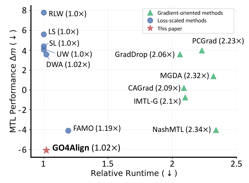
Figure 1: Performance and computational efficiency evaluation for MTO methods evaluated on NYUv2. Each method’s runtime is relative to a baseline method, which minimizes the sum of task-specific empirical risks. Left-down marks the comprehensive optimal results.

Multi-task learning is a promising paradigm for handling several tasks simultaneously using a unified architecture. It can achieve data efficiency, improve generalization, and bring a reduction in computation cost compared with addressing each task individually [48]. Due to these benefits, there is a growing surge of applications with multi-task learning in several domains, e.g., natural language processing [4, 38, 26], computer vision [48, 15, 27] and reinforcement learning [8, 42]. The crux of multi-task learning is to enable positive transfer among tasks while avoiding negative transfer, which usually exists among irrelevant tasks [49, 28, 44].

Existing Challenges: In avoiding the negative transfer, numerous multi-task optimization (MTO) methods [51, 15, 36, 49, 24] have emerged and attracted rising attention in recent years. A lasting concern in MTO is the task imbalance issue. It describes a phenomenon where some tasks are severely under-optimized [48], which can lead to worse overall performance with larger convergence differences across tasks.

To deal with the task imbalance issue, scaling methods are proposed for MTO. According to differences in scaling manipulations, we roughly divide MTO methods into gradient-oriented [51, 40, 23, 6, 39] and loss-oriented [15, 27, 20, 22]. The former tends to exhibit impressive results at the expense of higher computational or memory requirements during training time, due to the assessment of per-task gradients. In contrast, the latter preserves training-time efficiency but usually suffers from unsatisfactory overall performance. As shown in Fig. 1, most existing methods cannot simultaneously achieve superior performance and computational efficiency.

Proposed Solution: To improve the overall performance and maintain computational and memory efficiency, we propose Group Optimization for multi-task Alignment (GO4Align), a novel and effective loss-oriented method in MTO. As shown in Fig. 2, this work identifies multi-task alignment as a crucial factor in solving task imbalance, which means learning progress across tasks should synchronously achieve superior performance over all tasks. GO4Align dynamically aligns learning progress across tasks by exploiting group-based task interactions for multi-task empirical risk minimization. The rationale behind this idea is that groupings can implicitly capture task correlations for more effective multi-task alignment and thus help multi-task optimizers benefit from positive interactions among relevant tasks. The primary contribution is two-fold:

• As a new member of the loss-oriented branch, GO4Align recasts the task imbalance issue to a bi-level optimization problem, yielding an adaptive group risk minimization principle for MTO. Such a principle allocates weights over task losses at a group level to achieve learning progress alignment among relevant tasks.

• We develop a heuristic optimization pipeline in GO4Align to tractably achieve the principle, involving dynamical group assignment and risk-guided group indicators. The pipeline incorporates beneficial task interactions into the group assignments and exploits task correlations for multi-task alignment, improving the overall multi-task performance.

Experimental results show that our approach can outperform most existing state-of-the-art baselines in extensive benchmarks. Moreover, it does not sacrifice computational efficiency.

2 Preliminary

Notations. This work considers a multi-task problem over an input space $\mathcal{X}$ and a collection of task target spaces $\{\mathcal{Y}^{m}\}_{m=1}^{M}$, where $M\geq 2$ denotes the number of tasks. A composite dataset for multi-task learning is $\{({\bm{x}}_{n},y_{n}^{1},...,y_{n}^{M})\}_{n=1}^{N}$, where $N$ is the number of training samples. Let $\bm{\theta}^{s}$ and $\bm{\theta}^{m}$ respectively be the shared and task-specific parameters in a given multi-task model, thus we have a parametric hypothesis class for the $m$-th task as $f({\bm{x}}_{n};\bm{\theta}^{s},\bm{\theta}^{m}):\mathcal{X}\rightarrow\mathcal{Y}^{m}$. Then the empirical risk for the $m$-th task can be written as $\hat{\mathcal{L}}^{m}(\bm{\theta}^{s},\bm{\theta}^{m})=\frac{1}{N}\sum_{n=1}^{N}\ell^{m}(f({\bm{x}}_{n};\bm{\theta}^{s},\bm{\theta}^{m}),y_{n}^{m})$ , where $\ell^{m}(\cdot,\cdot):\mathcal{Y}^{m}\times\mathcal{Y}^{m}\rightarrow\mathbb{R}_{+}$ denotes the task-specific loss function. The ultimate goal of MTO is to achieve superior performance over all tasks.

Scale Empirical Risk Minimization (Scale-ERM). As preliminary, we recap a representative and related strategy in MTO, Scale-ERM, through the lens of risk minimization. Scale-ERM introduces a task-specific weight $\lambda^{m}\geq 0$ to scale the corresponding empirical risk. For conciseness, this principle is formulated using vector notations. Here, $\bm{\lambda}=\left[\lambda^{1},\lambda^{2},\cdots,\lambda^{M}\right]^{\top}\in\mathbb{R}^{M}$ represents a $M$-dimensional vector comprising all task-specific weights. And $\hat{\bm{L}}(\bm{\theta})=\left[\hat{\mathcal{L}}^{1}(\bm{\theta}^{s},\bm{\theta}^{1}),\hat{\mathcal{L}}^{2}(\bm{\theta}^{s},\bm{\theta}^{2}),\cdots,\hat{\mathcal{L}}^{M}(\bm{\theta}^{s},\bm{\theta}^{M})\right]^{\top}\in\mathbb{R}^{M}$ denotes the corresponding vector of empirical risks, where $\bm{\theta}=\{\bm{\theta}^{s},\bm{\theta}^{1},\bm{\theta}^{2},\cdots,\bm{\theta}^{M}\}$ represents all learnable parameters in a multi-task backbone network. Thus, we obtain the objective of Scale-ERM as follows:

$$\operatorname*{min}_{\bm{\theta},\bm{\lambda}}{\bm{\lambda}}^{\top}\hat{\bm{L}}({\bm{\theta}})+{\Omega}(\bm{\lambda}),$$ (1)

where ${\Omega}(\rm{\lambda})$ is a regularization term over task weights, designed to prevent the rapid collapse of these weights to zero, as discussed in Kendall et al. [15]. When all task weights are the same in scale, Scale-ERM will degenerate to the most simple strategy in MTO, where each task is treated equally during the joint training.

In Scale-ERM, each task weight controls task-specific learning progress, either by adapting the task-specific weights with loss information (loss-oriented) or by operating on task-specific gradients (gradient-oriented). As previously indicated, there still remains a research gap in MTO to improve multi-task performance without affecting computational efficiency.

3 Methodology

In resolving the task imbalance issue effectively and efficiently, we develop GO4Align in this section. Such an approach relies on grouping-based task interactions to align learning progress across tasks, which are specific to the loss-oriented branch to hold the advantage of computational efficiency.

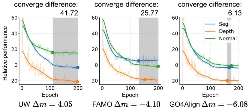
Figure 2: Multi-Task alignment and effects on performance. We visualize relative task performance curves (lower is better) over training epochs. Better overall performance usually occurs with lower convergence differences. Our method effectively reduces the convergence difference and achieves a better overall performance.

Motivation of Multi-Task Alignment. Empirically, we can observe that the overall performance is worse when there is a larger convergence difference. The convergence difference is measured by the standard deviation of the task-specific epoch numbers to arrive at convergence. As shown in Figure 2, UW [15] underperforms FAMO [24] in terms of a overall MTL metric $\Delta m\%$ (lower is better); while UW has a larger convergence difference than FAMO. Intuitively, a larger convergence difference means that per-task training dynamics are more asynchronous, usually leading to worse overall performance.

To perform MTO, we consider aligning tasks with group information in the multi-task risk minimization. We first present an adaptive group risk minimization principle for MTO, which targets the alignment of tasks’ learning progress from grouping-based task interactions. Then, in tractable problem-solving, we decompose the whole optimization process into two entangled phases: (i) dynamical group assignment and (ii) risk-guided group indicators. The pseudo-code of GO4Align is provided in Appendix B.

3.1 Adaptive Group Risk Minimization Principle

Recent advances [10, 14] have explored incorporating multi-task grouping in feature sharing and revealed its benefit of aligning the learning progress through task interactions. Nevertheless, their grouping mechanisms ignore monitoring the learning progress, e.g., failure to capture variations in loss scales among tasks, weakening the effectiveness of multi-task alignment.

As a result, we propose taking task-specific learning dynamics, which directly impact the convergence behaviors in optimization, into grouping mechanism design. This induces the adaptive group risk minimization principle suitable for multi-task alignment. The hypothesis is that the dynamical grouping tends to implicitly exploit task correlations [10] and encourages beneficial task interactions from empirical risk information along the learning progress. Meanwhile, such a principle retains computational efficiency as it avoids the computations of per-task gradients.

Adaptive Group Risk Minimization (AGRM). We achieve beneficial task interactions by producing task weights with a grouping mechanism, which is adaptive to various loss scales and their learning dynamics over time. Then, we recast the task imbalance issue with the grouping mechanism into a bi-level optimization problem: (i) In the lower-level optimization, the model aims to cluster $M$ tasks of interest into $K$ groups. This implicitly exploits task correlations, where similar tasks should be clustered into one group, yielding more beneficial task interactions. With group assignments, group weights are designed to conduct learning progress alignment at the group level. (ii) In the upper-level optimization, the proposed principle updates model parameters from the grouped empirical risks, which implicitly relies on the lower-level optimized results. We illustrate such a bi-level optimization with grouping-based task interactions in Fig. 3.

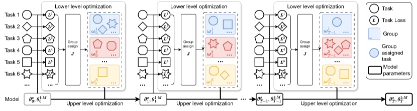
Figure 3: GO4Align using adaptive group risk minimization in the bi-level optimization framework. In the lower-level optimization, the model assigns tasks to groups with different group weights, encouraging task interactions and aligning learning progress. Such group information is nested into the upper-level optimization for updating the multi-task model’s parameters.

Given $K$ as the number of groups, we denote the assignment matrix as $\bm{\mathcal{G}}_{t}\in\mathbb{R}^{K\times M}$, where $\mathcal{G}_{t}(k,m)$ equals $1$ if the $k$-th group contains the $m$-th task and $0$ otherwise. Note that $\bm{\mathcal{G}}_{t}$ is updated in the optimization, with $t$-th indexing iteration step. The group number generally is smaller than the task number, e.g., $1<K\leq M$. To balance different groups, we place weights over groups $\bm{\omega}_{t}=\left[\omega_{t}^{1},\omega_{t}^{2},\cdots,\omega_{t}^{K}\right]^{\top}\in\mathbb{R}^{K}$, where $\omega_{t}^{k}\geq 0$ is specific to the $k$-th group at the $t$-th iteration. Formally, we formulate the bi-level optimization problem as:

$$\operatorname*{min}_{\bm{\theta}}{{{\bm{\omega}}_{t}}^{\top}}{\bm{\mathcal{G}}}_{t}\hat{\bm{L}}(\bm{\theta})~{}~{}~{}~{}\textit{s.t.}~{}\{{{\bm{\omega}}_{t}},{\bm{\mathcal{G}}}_{t}\}=\arg\operatorname*{min}_{\bm{\omega},\bm{\mathcal{G}}}\bm{J}(\bm{\omega},\bm{\mathcal{G}};\bm{\theta}_{t}),$$ (2)

where $\bm{\omega}_{t}$ and $\bm{\mathcal{G}}_{t}$ reflect adaptive group information in the lower-level optimization. $\bm{J}(\bm{\omega},\bm{\mathcal{G}};\bm{\theta}_{t})$ is the corresponding optimization objective for aligning the learning progress across tasks at the group levels, which is further explained in Sec. 3.2.

To be specific, we perform the bi-level optimization in Eq.(2) as the following steps. For the $t$-th iteration, we first compute the group information $\bm{\omega}_{t}$ and $\bm{\mathcal{G}}_{t}$ in the lower-level optimization; and then we update the model’s parameter in the upper-level optimization. As a result, we obtain the updated parameter $\bm{\theta}_{t+1}$, which is used to compute task-specific risk information at the next iteration. In the proposed principle, intra-group tasks share the same scaling weight $\omega^{k}\geq 0$ to prevent similar tasks from inconsistent learning progress, improving knowledge sharing among similar tasks.

Important in AGRM is to accommodate the grouping during training dynamically. In practice, the proposed principle is compatible with any gradient-based optimizer, such as SGD and Adam [16], yielding dynamical training for each task. As a new member of the loss-oriented branch, the grouping assignment matrix and group weights in GO4Align can sufficiently utilize the loss information over time to adaptively assign tasks and weight groups.

Unlike prior works on multi-task grouping [10, 14], which require group-specific architectures, our proposed principle focuses on group-specific scaling and adaptively executing grouping operations. These insights are: (i) the criteria for grouping tasks should take both learning dynamics and loss scales into consideration so that similar tasks can benefit from each other’s intermediate feature information and boost performance; (ii) adaptive grouping aligns learning progress across tasks and provides a more effective way for across-task information transfer.

3.2 Dynamical Group Assignment

In solving the optimization problem in Eq. (2), the main challenge lies in the involvement of discrete and continuous variables, which are implicitly entangled in the objective. In detail, the lower-level optimization requires adaptively adjusting the discrete variable $\bm{\mathcal{G}}_{t}$ and the continuous variable $\bm{\omega}_{t}$ for the learning progress alignment such that the model’s parameter $\bm{\theta}$ updates from the lastest grouping information.

Before executing the lower-level optimization, we need to introduce task-specific group indicators $\bm{\gamma}_{t}(\bm{\theta}_{t})=\left[\gamma^{1}_{t}({\bm{\theta}}_{t}^{s},{\bm{\theta}}_{t}^{1}),\gamma^{2}_{t}({\bm{\theta}}_{t}^{s},{\bm{\theta}}_{t}^{2}),\cdots,\gamma^{M}_{t}({\bm{\theta}}_{t}^{s},{\bm{\theta}}_{t}^{M})\right]^{\top}\in\mathbb{R}^{M}$. In general, this involves the entanglement of the model’s parameters, which is obtained from high-level optimization. These group indicators work for exploiting cross-task correlations along the learning progress and provide group information to enable task interactions in the lower-level optimization. We will further discuss the design of the group indicator in Sec. 3.3.

Intuitively, we conduct the group assignment as a clustering process based on these group indicators $\bm{\gamma}_{t}(\bm{\theta}_{t})$. In this case, each cluster represents a group, and the cluster center corresponds to the corresponding group weight. There exist numerous clustering algorithms available to achieve this, and this work takes the K-means clustering algorithm [19, 17, 1] as a practical clustering implementation. Next, we can specify the optimization objective of the dynamical group assignment as:

$$\min_{\bm{\omega},\bm{\mathcal{G}}}J(\bm{\omega},\bm{\mathcal{G}};\bm{\theta}_{t}):={||{\bm{\gamma}_{t}^{\top}}(\bm{\theta}_{t})-{\bm{\omega}^{\top}{\bm{\mathcal{G}}}}||}^{2},$$ (3)

where $\bm{\omega}_{t}^{\top}={\bm{\gamma}_{t}^{\top}}(\bm{\theta}_{t})\bm{\mathcal{G}}_{t}^{-1}$ indicates that the cluster center closely relates to the group assignment matrix. The designed dynamical group assignment plays an important role in the lower-level optimization of the proposed AGRM, and it tends to cluster similar tasks into the same group while scattering dissimilar ones in clusters.

By integrating the dynamical group assignment in Eq. (3) and the group indicators into Eq. (2), we can provide an instantiation for the AGRM’s optimization objective:

$$\operatorname*{min}_{\bm{\theta}}{{{\bm{\omega}}_{t}}^{\top}}{\bm{\mathcal{G}}}_{t}\hat{\bm{L}}(\bm{\theta})~{}\textit{s.t.}~{}\{{{\bm{\omega}}_{t}},{\bm{\mathcal{G}}}_{t}\}=\operatorname*{arg~{}min}_{{\bm{\omega}},\bm{\mathcal{G}}}{||{\bm{\gamma}_{t}^{\top}}(\bm{\theta}_{t})-{\bm{\omega}^{\top}{\bm{\mathcal{G}}}}||}^{2}.$$ (4)

Moreover, the dynamic group assignment heuristically clusters tasks from the group indicators, which avoids the exhausted search of appropriate task combinations for performance gains like previous works  [10].

3.3 Risk-guided Group Indicators

This subsection discusses the appropriate design of the group indicators for dynamic group assignment introduced in Sec. 3.2.

The misalignment of learning across tasks can usually be attributed to various risk scales and asynchronous learning dynamics among tasks over time. To address this, we take two operations, scale-balance and smooth-alignment, into consideration and then obtain the risk-guided group indicators by combining them.

Scale-balance. To alleviate the misalignment caused by differences in per-task risk scales, we introduce scale-balance, which enlarges the importance of tasks with smaller risks in optimization. Given task-specific risks at iteration $t$, we normalize them to their average risk for efficient scale balancing. In each iteration, the scale vector for all tasks is denoted as $\mathcal{P}_{t}(\bm{\theta}_{t})=\left[p_{t}^{1}(\bm{\theta}_{t}),p_{t}^{2}(\bm{\theta}_{t}),\dots,p_{t}^{M}(\bm{\theta}_{t})\right]^{\top}\in\mathbb{R}^{M}$, which can be calculated as:

$${\mathcal{P}_{t}(\bm{\theta}_{t})={\rm{diag}}(\hat{\bm{L}}(\bm{\theta}_{t}))^{-1}\Big{[}\bar{\hat{\bm{L}}}(\bm{\theta}_{t})\Big{]}_{M},}$$ (5)

where $\rm{diag}(\cdot)$ constructs a diagonal matrix with the elements of the vector placed on the diagonal. $\bar{\hat{\bm{L}}}(\bm{\theta}_{t})$ is a scalar to represent the average risk, and $[\cdot]_{M}$ represents the construction of an $M$-dimentional vector whose elements are all equal to the average risk. To avoid the upper-level optimization degenerating into a fixed scalar, the gradients of empirical risks in the lower-level optimization are not being computed through them. However, in practice, the learning dynamics over time tend to make the scale vector inconsistent over iterations [23, 51], which is not conducive to aligning learning progress. We therefore introduce smooth-alignment to update the scale vector with historical information from previous iterations.

Smooth-alignment. To avoid sudden fluctuations of scale vectors over iterations, we introduce the smoothness vector $\mathcal{Q}_{t}(\bm{\theta}_{1:t})=\left[q_{t}^{1}(\bm{\theta}_{1:t}),q_{t}^{2}(\bm{\theta}_{1:t}),\dots,q_{t}^{M}(\bm{\theta}_{1:t})\right]^{\top}\in\mathbb{R}^{M}$, which smooths the updating of the scale vector with previous risk information. Thus, the smoothness vector can deal with asynchronous learning dynamics over time, which helps the model to reduce the imbalance of training across tasks. To be specific, we compute the smoothness vector by a normalized exponential moving average as follows:

$$\mathcal{Q}_{t}(\bm{\theta}_{1:t}) =\sigma\Big{[}\bm{\mathcal{Q}}_{t-1}(\bm{\theta}_{1:t-1})\odot\exp(-\beta\hat{\bm{L}}(\bm{\theta}_{t}))\Big{]},$$ (6)

where $\odot$ denotes the element-wise multiplication and $\sigma[\cdot]$ normalizes the sum of all smoothness elements to be $1$. $\beta$ is a temperature hyperparameter to control the influence of previous grouping information. Note that when $\beta$ is close to zero, each element in the smoothness vector will degrade to a fixed value $\frac{1}{M}$, which does not capture any historical information to group indicators.

Risk-guided Group indicators. By integrating Eq. (5) and (6), we obtain the group indicators by:

$$\bm{\gamma}_{t}(\bm{\theta}_{t})={\mathcal{P}_{t}(\bm{\theta}_{t})\odot\mathcal{Q}_{t}(\bm{\theta}_{1:t})}.$$ (7)

Then, based on the group indicators $\bm{\gamma}_{t}(\bm{\theta}_{t})$ with scale-balance and smooth-alignment from risk information, we optimize the dynamical group assignment as Eq.(3) to assign tasks into groups in the lower-level optimization.

For each group indicator, the role of $\mathcal{P}_{t}(\bm{\theta}_{t})$ in Eq. (5) and $\mathcal{Q}_{t}(\bm{\theta}_{1:t})$ in Eq. (6) differs in optimization: the smoothness vector requires the accumulated loss information from previous iterations, while the scale vector are independent of iterations. Thus, the smoothness vector can iteratively exploit more consistent task correlations to better align learning progress across tasks. The experimental section will show that the risk-guided group indicators empirically boost the proposed adaptive group risk minimization in aligning learning tasks.

4 Related Work

Multi-Task Optimization. Multi-task optimization aims to address the task imbalance issue in multi-task learning, where each task usually has a different influence on a shared network. According to different inductive biases, we can roughly divide multi-task optimization methods into two branches: (i) Gradient-oriented methods, which solve the task balancing problem by fully utilizing the gradient information of the shared network from different tasks. Some studies report impressive performance based on Pareto optimal solutions [39], gradient normalization [5], gradient conflicting [51], gradient sign Dropout [6], conflict-averse gradient [23], Nash bargaining solution [36]. However, most gradient manipulation methods usually suffer from high computational cost [20]. (ii) Loss-oriented methods, which reweight task-specific losses with the help of inductive biases from the loss space, e.g., using homoscedastic uncertainty [15], task prioritization [12], self-paced learning [34], similar learning paces [27, 24], random loss weight [22]. Although loss-oriented methods are more computationally efficient, they often underperform gradient-oriented ones in most multi-task benchmarks. GO4Align in this work tries to trade off the overall performance and computational efficiency.

Recent work [37] weights tasks under the meta-learning setup but has lower training-time efficiency for large-scale systems with high dimensional parameter space, such as deep neural networks, limiting their applications for dense prediction tasks in MTL. The closest method to ours is the recent work FAMO [24], which balances task-specific losses by decreasing task loss approximately at an equal rate. However, GO4Align proposes a new MTL optimizer that dynamically aligns learning progress across tasks by introducing group-based task interactions.

Multi-Task Grouping. Multi-task grouping [44, 43, 10] assigns tasks into different groups and trains intra-group tasks together in a shared multi-task network. Previous work [44] first evaluates the transferring gains for $2^{M}-1$ candidate multi-task networks ($M$ is the number of tasks) and then conducts the brute-force search for the best grouping. Some works follow high-order approximation (HOA) [44] to reduce the prohibitive computational cost. However, they also suffer from inaccurate estimations due to non-linear relationships between high-order gains and corresponding pairwise gains [43]. Meanwhile, Yao et al. [50] represents a clustered multi-task learning method, which clusters tasks into several groups by learning the representative tasks. The benefit of multi-task grouping is performance gains by training similar tasks together, and this inspires us to capture helpful group information in multi-task optimization. Also, rather than employing different multi-task networks, GO4Align introduce group-based task interactions in scaling for multi-task alignment. Moreover, we share a high-level idea of task clustering with  [46]. However, task clustering in  [46] is limited to pairwise relationships among tasks. However, our work allows grouping-based task interactions, thus capturing more complex relationships among tasks.

5 Experiment

5.1 Multi-Task Supervised Learning

Datasets and Settings. We conduct experiments on four benchmarks commonly used in multi-task optimization literature [24, 23, 27, 36]. These include NYUv2 [35], CityScapes [7], QM9 [3], and CelebA [29]. For all benchmarks, we follow the training and evaluation protocol in [36, 24]. Detailed information about experimental results and baselines is in Appendix C.

Baselines. We compare GO4Align with a single-task learning baseline, $6$ gradient-oriented methods, and $6$ loss-oriented methods. Note that single-task learning (STL) trains an independent deep network for each task. The gradient-oriented methods include MGDA [39], PCGrad [51], CAGrad [23], IMTL-G [25], GradDrop [6], and NashMTL [36]. As for the loss-oriented methods, they are Linear scalarization (LS), Scale-invariant (SI), Dynamic Weight Average (DWA) [27], Uncertainty Weighting (UW) [15], Random Loss Weighting (RLW) [21], and FAMO [24].

	Segmentation		Depth		Surface Normal
Method	mIoU $\uparrow$	Pix Acc $\uparrow$	Abs Err $\downarrow$	Rel Err $\downarrow$	Angle Dist $\downarrow$		Within $t^{\circ}$ $\uparrow$			MR $\downarrow$	$\Delta m\%$ $\downarrow$
					Mean	Median	11.25	22.5	30
STL	38.30	63.76	0.6754	0.2780	25.01	19.21	30.14	57.20	69.15	-	-
MGDA	30.47	59.90	0.6070	0.2555	24.88	19.45	29.18	56.88	69.36	7.00	1.38
PCGrad	38.06	64.64	0.5550	0.2325	27.41	22.80	23.86	49.83	63.14	9.00	3.97
GradDrop	39.39	65.12	0.5455	0.2279	27.48	22.96	23.38	49.44	62.87	7.89	3.58
CAGrad	39.79	65.49	0.5486	0.2250	26.31	21.58	25.61	52.36	65.58	5.33	0.20
IMTL-G	39.35	65.60	0.5426	0.2256	26.02	21.19	26.20	53.13	66.24	4.56	-0.76
NashMTL	40.13	65.93	0.5261	0.2171	25.26	20.08	28.40	55.47	68.15	2.89	-4.04
LS	39.29	65.33	0.5493	0.2263	28.15	23.96	22.09	47.50	61.08	9.89	5.59
SI	38.45	64.27	0.5354	0.2201	27.60	23.37	22.53	48.57	62.32	8.78	4.39
RLW	37.17	63.77	0.5759	0.2410	28.27	24.18	22.26	47.05	60.62	12.22	7.78
DWA	39.11	65.31	0.5510	0.2285	27.61	23.18	24.17	50.18	62.39	8.67	3.57
UW	36.87	63.17	0.5446	0.2260	27.04	22.61	23.54	49.05	63.65	8.33	4.05
FAMO	38.88	64.90	0.5474	0.2194	25.06	19.57	29.21	56.61	68.98	4.33	-4.10
GO4Align	40.42	65.37	0.5492	0.2167	24.76	18.94	30.54	57.87	69.84	2.11	-6.08

Table 1: Results on NYUv2 dataset (3 tasks). The upper and lower tables categorize baseline methods into gradient-oriented and loss-oriented types, respectively. Each experiment is repeated over 3 random seeds and the mean is reported. The best average result is marked in bold. MR and $\Delta m\%$ are the main metrics for MTL performance.

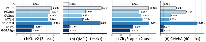
Figure 4: Efficiency comparisons on training time. Each method’s runtime is relative to a baseline method with Eq.(1), which minimizes the sum of task-specific empirical risks.

Evaluations. Following previous works [36, 32, 23], we report two MTL metrics that demonstrate the overall performance over various task-specific metrics: (1) $\Delta m\%$ is the average per-task performance drop relative to STL. We assume there are $S$ metrics for all tasks. $\mathcal{M}^{s}$ denote the $s$-th metric value of a multi-task method, while $\mathcal{B}^{s}$ is the corresponding metric value of the STL baseline. Thus, we formulate the average relative performance drop as:${\bm{\Delta m}}\%=\frac{1}{S}\sum_{s=1}^{S}(-1)^{\delta^{s}}\frac{(\mathcal{M}^{s}-\mathcal{B}^{s})}{\mathcal{B}^{s}}$, where ${\delta^{s}}=1$ if higher values for the $s$-th metric are better and $0$ otherwise. (2) ${\textbf{MR}}{}=\frac{1}{S}\sum_{s=1}^{S}\text{rank}(\mathcal{M}^{s})$ is the average rank of all task-specific metrics, where $\text{rank}(\mathcal{M}^{s})$ denotes the ranking of the $s$-th metric value of the model among all comparison methods. Note that in practice the lower $\Delta m\%$ and MR, the better overall performance.

Method	QM9		CityScapes		CelebA
	MR $\downarrow$	$\Delta m\%$ $\downarrow$	MR $\downarrow$	$\Delta m\%$ $\downarrow$	MR $\downarrow$	$\Delta m\%$ $\downarrow$
MGDA	7.73	120.5	10.00	44.14	10.05	14.85
PCGrad	6.09	125.7	6.25	18.29	6.05	3.17
CAGrad	7.09	112.8	5.00	11.64	5.65	2.48
IMTL-G	5.91	77.2	4.00	11.10	4.08	0.84
NashMTL	3.64	62.0	2.50	4.28	4.53	2.84
LS	8.00	177.6	8.50	14.11	5.55	4.15
SI	5.09	77.8	8.50	14.11	7.10	7.20
RLW	9.36	203.8	7.75	24.38	4.60	1.46
DWA	7.64	175.3	6.00	21.45	6.25	3.20
UW	6.64	108.0	5.75	5.50	5.18	3.23
FAMO	4.73	58.5	5.50	8.13	4.10	1.21
GO4Align	4.55	52.7	7.00	8.11	3.10	0.88

Table 2: Comparisons on QM9 (11 tasks), CityScapes (2 tasks) and CelebA (40 tasks). Detailed results are in Appendix D.

Effectiveness Comparisons. We provide performance comparisons on NYUv2 in Table 1. In this benchmark, our method achieves the best performance, in terms of the average performance drop, among both gradient-oriented and loss-oriented methods. Especially we find that our work is the only one that improves each task’s performance relative to the corresponding STL performance. This suggests that grouping-based task interactions can adequately alleviate the imbalance of learning progress across tasks.

The experimental results on QM9, CityScapes and CelebA are reported in Table 2. GO4Align obtains the lowest $\Delta m\%$ on QM9. It also shows comparable performance with FAMO on CityScapes, one possible reason could be that this dataset only contains $2$ tasks, which limits the potential of the grouping mechanism in our method. In CelebA, even though our work does not achieve the lowest average performance drop, it outperforms all loss-oriented methods, which further verifies the effectiveness of the proposed method.

Efficiency Comparisons. To show the computational efficiency, in Fig. 4, we report the average training time per epoch over 5 random epochs of the proposed methods and baseline methods. We note that we run all experiments on an NVIDIA A100 and the code of baseline methods comes from  Liu et al. [24] and  Navon et al. [36]. As shown in this figure, the proposed method GO4Align, as a new member of the loss-oriented branch, can perform more efficiently than most gradient-oriented methods. Moreover, we observe that the training time of gradient-oriented methods is proportional to the number of tasks, but our work can avoid this.

5.2 Ablation Studies

The effectiveness and efficiency of the proposed method are shown in Sec. 5.1. Next, the goal of our ablation study is to answer the following questions: (1) Can we quantify the contributions of each phrase? (2) Can we disentangle the roles of the group assignment and group weights? (3) Are there practical ways to appropriately configure hyperparameters, e.g., group number $K$?

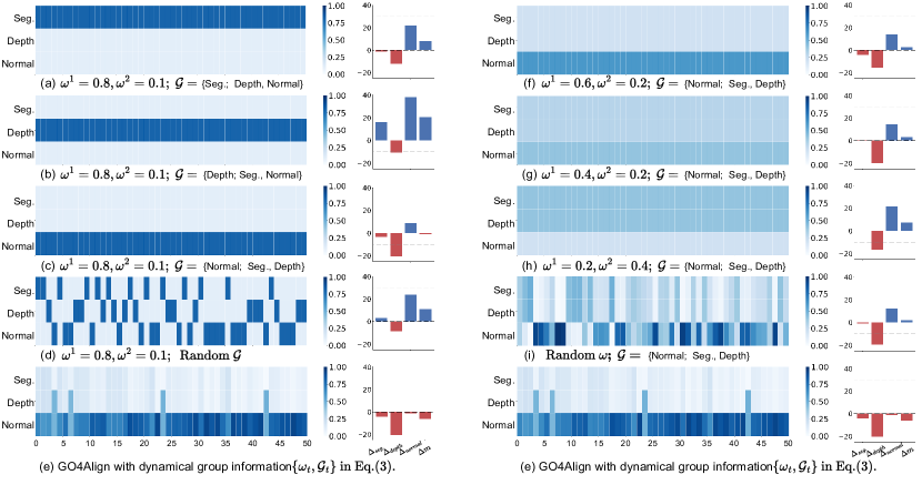
Figure 5: Comparative analysis of the influence of group assignment and weights in the proposed AGRM principle on NYUv2. The number of groups is $2$. (a-d) have a fixed group weight $\bm{\omega}=[\omega^{1},\omega^{2}]$ but various group assignments $\mathcal{G}$ to show the influence of group assignment. (f-i) have various group weights $\bm{\omega}$ but a fixed group assignment $\mathcal{G}$ to show the influence of group weights. (e) is our method, that exploits dynamical group information from bi-level optimization. The right side of each method shows relative performance drops on each task and the average performance drop.

Eq.(5)	Eq.(6)	Eq.(4)	$\bm{\Delta}_{seg.}\%$ $\downarrow$	$\bm{\Delta}_{depth}\%$ $\downarrow$	$\bm{\Delta}_{normal}\%$ $\downarrow$	$\Delta m\%$ $\downarrow$
✓			-0.02	-21.76	13.14	2.46
✓	✓		14.22	-15.27	2.52	1.16
✓	✓	✓	-4.03	-20.37	-1.18	-6.08

Table 3: Effectiveness of each phase in GO4Align on NYUv2. ✓ denote whether the component joins the pipeline.

Contributions of Each Phase. To quantify the contributions of each phase in achieving the proposed AGRM principle on NYUv2, we report the detailed performance of our method in each phase. As shown in Table 3, compared with the scale vector in Eq. (5), the smoothness vector in Eq. (6) can compromise the performance of the “normal” and “depth” tasks, however, scarifying that of “seg.”. Based on the scale and smoothness vectors, the proposed method employs dynamical group assignment in Eq.(4) to exploit the grouping-based task interactions, thus well aligning the learning progress of similar tasks “depth” and “seg.”. We also observe that our method with both phases can improve the task-specific performance relative to STL. This demonstrates that each phase in the method complements each other, resulting in more balanced performance across tasks.

Influence of Group Assignment. To explore the influence of the group assignment matrix in the proposed AGRM principle, we assume $K=2$ on NYUv2 and make comparisons with several variants, which have various group assignments with fixed group weights. In Fig. 5, (a-c) are three fixed grouping options, e.g., (a) groups “depth" and “normal" tasks and set the group weight as $0.1$.

As shown in this figure, even with fixed group weights, the appropriate group assignment shows impressive performance. In particular, grouping “Seg." and “Depth" outperforms other options. The main reason could be these two tasks are very similar to each other and far away from the “normal” task [10]. We observe that variant (d) with a random grouping strategy shows lower performance than the fixed grouping options (a) and (c), which further implies the importance of appropriate group assignment in AGRM. It is worth mentioning that the proposed method in (e) without the prior information of the appropriate group assignment also captures such task correlations and each task can get performance gains compared with STL. This demonstrates that group assignment plays an important role in exploring task correlations over time in the proposed AGRM principle.

Influence of Group Weights. To study the influence of group weights in AGRM, we conduct another visualization in Fig. 5 (f-i), where we focus on various group weights with the “optimal" group assignment. (f-h) are three fixed grouping weights, e.g., (f) weight the “Normal" task in the first group with $0.6$ and weight the “Seg.” and “Depth" tasks in the second group with $0.2$. For a clear comparison, we normalize the sum of all weights to $1$.

We observe that with the fixed grouping option, group weights have effects on the extent of compromising among different groups. On the NYUv2 dataset, lower weights for the first groups obtain better overall performance. The variant method (i) with random group weights achieves surprising performance, $1.75\%$, in terms of the average relative performance drop. (e) shows that our method also tends to dynamically weight the first group with a high value. This demonstrates that group weights are necessary to align the learning progress of different groups over time in the proposed AGRM principle.

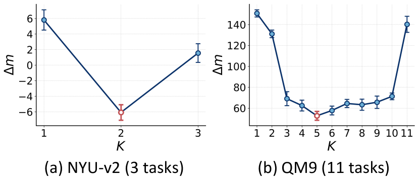
Figure 6: Identification of “elbow” points on NYUv2 (a) and QM9 (b). According to the conventional elbow method, we set the group number of the two datasets as 2 and 5, respectively.

Influence of Group Number. In the proposed method, group number $K$ is an important hyper-parameter, especially when we instantiate the clustering process in dynamical group assignment with $K$-means. In this case, there are many different techniques for choosing the right $K$. To be visualizable, here we apply the conventional elbow method. As shown in Fig. 6, the overall performance (lower is better) of our method in (a) and (b) drops at $2$ and $5$, respectively, after that both reach a plateau when the group numbers increase. Thus, in this paper we set $K=2$ and $K=5$ for NYUv2 and QM9.

6 Conclusion

Technical Discussion. This paper focuses on the task imbalance issue in MTO. Previous MTO methods suffer from either intensive computations or non-competitive performance. Our proposed GO4Align addresses the issue by aligning learning progress across tasks with the help of the AGRM principle. In problem-solving, we present a tractable optimization pipeline, which incorporates grouping-based task interactions into the loss scaling of MTO.

Limitation. The main limitation of this work is the heuristic configuration of the group numbers. Although the search space is significantly smaller than some grouping multi-task methods [43], it still needs maximum $M$ runs to find the best number. Some related techniques [41] automatically set the group number can be added to avoid this limitation in future work.

Broader Impact. This paper is the first to consider task grouping in multi-task optimization with deep multi-task models. We propose a simple and principled way to fasten multi-task optimization with lower training-time efficiency, which has many potential societal impacts, especially in dense prediction tasks.

Appendix A Related Work on Deep Multi-task Architecture

In this section, we group multi-task learning methods into three categories: multi-task optimization, multi-task grouping, and deep multi-task architecture. The first two categories are most related to this paper and are mentioned in the main paper. To be self-contained, here we provide detailed discussions about deep multi-task architecture.

Our method GO4Align builds on multi-task grouping and multi-task optimization, inheriting advantages from both to balance different tasks in joint learning. In the following, we discuss each category of multi-task learning methods and explain how it relates to our proposed method.

Deep Multi-Task Architecture. Multi-task architecture design can be roughly categorized into either a hard-parameter sharing design [18, 31] or a soft-parameter sharing design [33, 11, 27]. The hard-parameter sharing design generally contains a shared encoder and several task-specific decoders. Branching points between the shared encoder and decoders are determined in an ad-hoc way [48, 47], resulting in a suboptimal solution. Some work [13, 31, 45] automatically learns where to share or branch with a network. The soft-parameter sharing design considers all parameters task-specific and instead learns feature-sharing mechanisms to handle the cross-task interactions [33, 30]. Soft-parameter sharing methods usually struggle with model scalability as the model size grows linearly with the number of tasks. GO4Align focuses on the optimization of multi-task learning, which adopts a simple hard-parameter sharing architecture as the backbone and subsequently reduces task interference in the gradient space of the shared encoder or the loss space.

Appendix B Algorithm

The pseudo-code of GO4Align is provided in Algorithm 1. For the sake of clarity, we also illustrate the optimization process in Fig. 7.

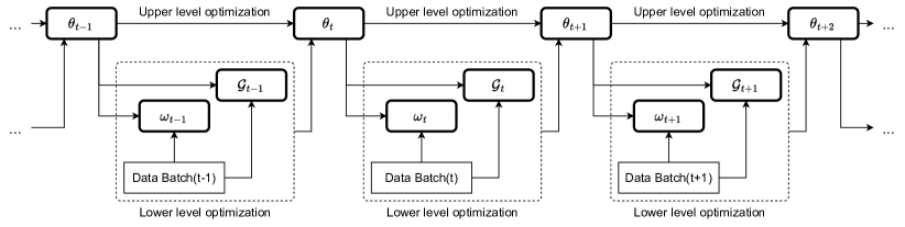
Figure 7: Optimization process of the proposed adaptive group risk minimization principle. At each iteration, given the randomly sampled mini-batch data, we first compute the group information $\bm{\omega}$ and $\bm{\mathcal{G}}$ in the lower-level optimization and then update the model’s parameter in the upper-level optimization.

Algorithm 1 Group Optimization for Multi-Task Alignment (GO4Align)

1:  Input: Maximum iteration number $T$; Batch size $N_{\rm{bz}}$; Learning rate $\alpha$; Temperature hyperparameter $\beta$; Task number $M$; Group number $(1<K\leq M)$; Calibration vector $\bm{\mathcal{Q}}(\bm{\theta})$.

2:  Initialize model parameters $\bm{\theta}_{0}=\{\bm{\theta}^{s}_{0},\bm{\theta}^{1}_{0},\bm{\theta}^{2}_{0},\cdots,\bm{\theta}^{M}_{0}\}$;

3:  Initialize each calibration value $q^{m}_{0}\leftarrow{\frac{1}{M}}$;

4:  for $t=0:T$ do

5:     Randomly sample a batch of training samples: $\{({\bm{x}}_{n},y_{n}^{1},...,y_{n}^{M})\}_{n=1}^{N_{\rm{bz}}},\text{where}~{}\bm{x}_{n}\in\mathcal{X},y_{n}^{m}\in\mathcal{Y}^{m};$

6:     Compute the empirical risk for each task at the $t$-th iteration: $\hat{\mathcal{L}}^{m}(\bm{\theta}^{s}_{t},\bm{\theta}^{m}_{t})=\frac{1}{N_{\rm{bz}}}\sum_{n=1}^{N_{\rm{bz}}}\ell^{m}(f({\bm{x}}_{n};\bm{\theta}^{s}_{t},\bm{\theta}^{m}_{t}),y_{n}^{m});$ // Lower-level optimization for grouping-based task interactions.

7:     Compute the scale vector ${{\mathcal{P}}_{t}(\bm{\theta}_{t})}$ in Eq. (5);

8:     Compute the smoothness vector ${{\mathcal{Q}}_{t}(\bm{\theta}_{1:t})}$ in Eq. (6);

9:     Obtain the group indicators ${\gamma}_{t}(\bm{\theta}_{1:t})$ with Eq.(7);

10:     Update the group information $\bm{\omega}_{t}$ and $\bm{\mathcal{G}}_{t}$ with Eq. (3) and the obtained ${\gamma}_{t}(\bm{\theta}_{1:t})$. // Upper-level optimization for model parameters.

11:     Update the model parameters $\bm{\theta}$ with Eq. (4): $\bm{\theta}_{t+1}\leftarrow\operatorname*{argmin}_{\bm{\theta}}{{{\bm{\omega}}_{t}}^{\top}}{\bm{\mathcal{G}}}_{t}\hat{\bm{L}}(\bm{\theta}).$

12:  end for

Appendix C Experimental Set-Up & Implementation Details

C.1 Benchmark Descriptions

NYUv2 [35] is an indoor scene dataset consisting of 1449 RGBD images and dense per-pixel labeling with 13 classes. The learning objectives include $3$ different dense prediction tasks: image segmentation, depth prediction, and surface normal prediction based on any scene image.

CityScapes [7] contains 5000 street-view RGBD images with per-pixel annotations. It needs to predict $2$ dense prediction tasks: image segmentation and depth prediction.

QM9 [3] is a benchmark for group neural networks to predict $11$ properties of molecules. It consists of $>$130K molecules represented as graphs annotated with node and edge features. We use $110K$ molecules from the QM9 example in PyTorch Geometric [9], $10K$ molecules for validation, and the rest of $10K$ molecules as a test set.

CelebA [29] contains 200K face images of 10K different celebrities, and each face image is provided with 40 facial binary attributes. As the protocol provided in previous work [24], each attribute corresponds to one task. Thus, we consider CelebA as a 40-task MTL problem.

C.2 Compared Multi-task Learning Baselines

From the gradient manipulation branch, (1) MGDA [39] that finds the equal descent direction for each task; (2) PCGrad [51] proposes to project each task gradient to the normal plan of that of other tasks and combining them together in the end; (3) CAGrad [23] optimizes the average loss while explicitly controls the minimum decrease across tasks; (4) IMTL-G [25] finds the update direction with equal projections on task gradients; (5) GradDrop [6] that randomly dropout certain dimensions of the task gradients based on how much they conflict; (6) NashMTL [36] formulates MTL as a bargaining game and finds the solution to the game that benefits all tasks.

From the loss scaling branch, (1) Linear scalarization (LS) is the sum of empirical risk minimization; (2) Scale-invariant (SI) is invariant to any scalar multiplication of task losses; (3) Dynamic Weight Average (DWA) [27], a heuristic for adjusting task weights based on rates of loss changes; (4) Uncertainty Weighting (UW) [15] uses task uncertainty as a proxy to adjust task weights; (5) Random Loss Weighting (RLW) [21] that samples task weighting whose log-probabilities follow the normal distribution; (6) FAMO [24] decreases task losses approximately at equal rates.

C.3 Neural Architectures & Training Details

For NYUv2 and CityScapes, we follow the training and evaluation protocol in [36], which adds data augmentations during training for all compared methods. We train each method for 200 epochs with an initial learning rate of $1e-4$ and reduce the learning rate to $5e-5$ after 100 epochs. The architecture is Multi-Task Attention Network (MTAN) [27] built upon SegNet [2]. Batch sizes for NYUv2 and CityScapes are set as 2 and 8 respectively. To make a fair comparison with previous works [27, 23, 24, 51], we report the test performance averaged over the last 10 epochs.

We follow the protocol in  Navon et al. [36] to normalize each task target at the same scale for fairness. We train each method for 300 epochs with a batch size of 120 and search for the best learning rate in ${\{1e-3,5e-4,1e-4\}}$. We take ReduceOnPlateau [36] as the learning-rate scheduler to decrease the lr once the validation overall performance stops improving. The validation set is also used for early stopping.

Following [24], we use a neural network with five convolutional and two fully connected layers as the shared encoder. The decoder of each task is implemented by another fully connected layer. We train the model for 15 epochs with a batch size of 256. We adopt Adam as the optimizer with a fixed learning rate of $1e-3$. Similar to QM9, we use the validation set for early stopping and hyperparameter selection, such as the number of groups $K$ and the step size of smoothness value $\beta$. We conduct all experiments on a single NVIDIA A100 GPU.

Appendix D Additional Experimental Results

D.1 Detailed results on QM9 and CityScapes

We provide task-specific performance on QM9 in Table 4. The proposed GO4Align obtains the best performance in terms of the average performance drop $\Delta m\%$. And its average rank MR is lower than all loss-oriented methods, which demonstrates the proposed method can get a more balanced performance for each task.

As shown in Table 5, our method achieves competitive performance on CityScapes with other alternatives except for NashMTL and UW. The main reason can be that there are only two tasks in the datasets, which constrains the effectiveness of the grouping mechanism in our method.

Method	$\mu$	$\alpha$	$\epsilon_{\text{HOMO}}$	$\epsilon_{\text{LUMO}}$	$\langle R^{2}\rangle$	ZPVE	$U_{0}$	$U$	$H$	$G$	$c_{v}$	MR $\downarrow$	$\Delta m\%$ $\downarrow$
	MAE $\downarrow$
STL	0.07	0.18	60.6	53.9	0.50	4.53	58.8	64.2	63.8	66.2	0.07	-	-
MGDA	0.22	0.37	126.8	104.6	3.23	5.69	88.4	89.4	89.3	88.0	0.12	7.73	120.5
PCGrad	0.11	0.29	75.9	88.3	3.94	9.15	116.4	116.8	117.2	114.5	0.11	6.09	125.7
CAGrad	0.12	0.32	83.5	94.8	3.22	6.93	114.0	114.3	114.5	112.3	0.12	7.09	112.8
IMTL-G	0.14	0.29	98.3	93.9	1.75	5.70	101.4	102.4	102.0	100.1	0.10	5.91	77.2
NashMTL	0.10	0.25	82.9	81.9	2.43	5.38	74.5	75.0	75.1	74.2	0.09	3.64	62.0
LS	0.11	0.33	73.6	89.7	5.20	14.06	143.4	144.2	144.6	140.3	0.13	8.00	177.6
SI	0.31	0.35	149.8	135.7	1.00	4.51	55.3	55.8	55.8	55.3	0.11	5.09	77.8
RLW	0.11	0.34	76.9	92.8	5.87	15.47	156.3	157.1	157.6	153.0	0.14	9.36	203.8
DWA	0.11	0.33	74.1	90.6	5.09	13.99	142.3	143.0	143.4	139.3	0.13	7.64	175.3
UW	0.39	0.43	166.2	155.8	1.07	4.99	66.4	66.8	66.8	66.2	0.12	6.64	108.0
FAMO	0.15	0.30	94.0	95.2	1.63	4.95	70.82	71.2	71.2	70.3	0.10	4.73	58.5
GO4Align	0.17	0.35	102.4	119.0	1.22	4.94	53.9	54.3	54.3	53.9	0.11	4.55	52.7

Table 4: Detailed results on  QM9. Each experiment is repeated over 3 random seeds and the mean is reported. The best average result is marked in bold. MR and $\Delta m\%$ are the main metrics for MTL performance.

Method	Segmentation		Depth		MR $\downarrow$	$\Delta m\%$ $\downarrow$
	mIoU $\uparrow$	Pix Acc $\uparrow$	Abs Err $\downarrow$	Rel Err $\downarrow$
STL	74.01	93.16	0.0125	27.77
MGDA	68.84	91.54	0.0309	33.50	10.00	44.14
PCGrad	75.13	93.48	0.0154	42.07	6.25	18.29
CAGrad	75.16	93.48	0.0141	37.60	5.00	11.64
IMTL-G	75.33	93.49	0.0135	38.41	4.00	11.10
NashMTL	75.41	93.66	0.0129	35.02	2.50	6.82
LS	70.95	91.73	0.0161	33.83	8.50	14.11
SI	70.95	91.73	0.0161	33.83	8.50	14.11
RLW	74.57	93.41	0.0158	47.79	7.75	24.38
DWA	75.24	93.52	0.0160	44.37	6.00	21.45
UW	72.02	92.85	0.0140	30.13	5.75	5.50
FAMO	74.54	93.29	0.0145	32.59	5.50	8.13
GO4Align	72.63	93.03	0.0164	27.58	7.00	8.11

Table 5: Detailed results on  CityScapes. Each experiment is repeated over 3 random seeds and the mean is reported. The best average result is marked in bold. MR and $\Delta m\%$ are the main metrics for MTL performance.

D.2 Training time comparisons

In Fig. 4, we show the training time of MTO methods relative to a baseline method (LS). Here we provide real training time (seconds) in Table 6, where we compute the average training time of randomly 5 epochs. From this table, we observe that loss-oriented methods in general use less time for one epoch than gradient-oriented methods. GO4Align requires the second lowest time cost during training on all four datasets, demonstrating its good computational efficiency.

Method	NYU-v2	QM9	CityScapes	CelebA
MGDA	199.73	601.52	136.69	902.53
PCGrad	192.41	352.05	100.21	1486.71
CAGrad	180.37	296.36	107.84	590.05
IMTL-G	180.67	306.11	113.51	522.22
NashMTL	201.30	585.37	138.26	2134.75
LS	86.21	88.95	66.63	170.81
FAMO	102.87	100.40	78.70	183.46
GO4Align	87.78	93.50	67.30	171.69

Table 6: Detailed training time (seconds) for one epoch of different methods. In addition to LS, our method requires the lowest time cost during training on all 4 datasets.

D.3 Visualizations on risk ratios

To investigate the influence of different scaling methods on the training of tasks, we illustrate the ratios between task-specific empirical risk and the sum of all empirical risks before and after scaling on NYUv2. In each small figure, the three shadows from top to down represent the ratios of “normal”, “seg.” and “depth”, respectively. The x-axis represents epochs ranging from $1$ to $200$. Note that MGDA and NashMTL scale task-specific gradients. For direct comparisons, here we provide the scaled loss ratios, which are equivalent to gradient scaling for the shared network.

As shown in Fig. 8, all methods have similar ratios over epochs on the unscaled risks but perform differently on the scaled risks. We observe that MGDA have a significantly larger ratio on the “normal” task, which means MGDA prefers to optimize the “normal” task. Compared with related works, our method has more stable ratios of different tasks. The possible reason could be that our method benefits from historical information, which avoids training instability among tasks.

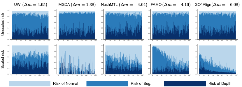
Figure 8: Analysis on risk ratios. Compared with other works, the proposed GO4Align shows more stable ratios among tasks over epochs, indicating that GO4Align can maintain better alignment throughout the training process.

D.4 Dynamical group assignment with different group indicators

To tractably solve the bi-level problem in the introduced adaptive group risk minimization principle, we decompose the whole optimization process into two entangled phases: (i) dynamical group assignment and (ii) risk-guided group indicator. In addition to the designed group indicator, the adaptive group risk minimization can also be plug-and-play in previous methods by utilizing their learnable task weights as the group indicators.

The results of previous methods (MGDA [39], NashMTL [36], and FAMO [24]) with the proposed adaptive group risk minimization are reported in Table 7. The experiments are conducted on NYU-v2. As shown in the table, when combined with the adaptive group risk minimization, the previous methods further improve the overall performance. MGDA with adaptive group risk minimization achieves the most obvious improvement. Moreover, our method still outperforms the other methods. The reason can be our group indicator considers both the inter-task and historical information, whereas the task scales of other methods do not.

Methods	$\bm{\Delta}_{seg.}\%$ $\downarrow$	$\bm{\Delta}_{depth}\%$ $\downarrow$	$\bm{\Delta}_{normal}\%$ $\downarrow$	$\bm{\Delta}_{m}\%$ $\downarrow$
MGDA	13.25	-9.11	0.83	1.38
MGDA+Sec.3.2(Ours)	6.06	-11.69	-1.14	-1.89
NashMTL	-4.09	-22.01	3.15	-4.04
NashMTL+Sec.3.2(Ours)	-7.75	-20.14	3.60	-4.20
FAMO	-1.65	-20.02	1.29	-4.10
FAMO +Sec.3.2(Ours)	1.76	-21.17	-0.03	-4.32
Sec.3.3(Ours)+Sec.3.2(Ours)	-4.03	-20.37	-1.18	-6.08

Table 7: Adaptive group risk minimization with different group indicators. With the adaptive group risk minimization, previous methods perform better on the overall results. Moreover, our method still performs the best compared with the others.

References

- Ahmed et al. [2020] Ahmed, M., Seraj, R., and Islam, S. M. S. The k-means algorithm: A comprehensive survey and performance evaluation. Electronics, 9(8):1295, 2020.
- Badrinarayanan et al. [2017] Badrinarayanan, V., Kendall, A., and Cipolla, R. Segnet: A deep convolutional encoder-decoder architecture for image segmentation. IEEE transactions on pattern analysis and machine intelligence, 39(12):2481–2495, 2017.
- Blum & Reymond [2009] Blum, L. C. and Reymond, J.-L. 970 million druglike small molecules for virtual screening in the chemical universe database GDB-13. J. Am. Chem. Soc., 131:8732, 2009.
- Chen et al. [2021] Chen, S., Zhang, Y., and Yang, Q. Multi-task learning in natural language processing: An overview. arXiv preprint arXiv:2109.09138, 2021.
- Chen et al. [2018] Chen, Z., Badrinarayanan, V., Lee, C.-Y., and Rabinovich, A. Gradnorm: Gradient normalization for adaptive loss balancing in deep multitask networks. In International Conference on Machine Learning, pp. 794–803. PMLR, 2018.
- Chen et al. [2020] Chen, Z., Ngiam, J., Huang, Y., Luong, T., Kretzschmar, H., Chai, Y., and Anguelov, D. Just pick a sign: Optimizing deep multitask models with gradient sign dropout. arXiv preprint arXiv:2010.06808, 2020.
- Cordts et al. [2016] Cordts, M., Omran, M., Ramos, S., Rehfeld, T., Enzweiler, M., Benenson, R., Franke, U., Roth, S., and Schiele, B. The cityscapes dataset for semantic urban scene understanding. In Proceedings of the IEEE conference on computer vision and pattern recognition, pp. 3213–3223, 2016.
- Espeholt et al. [2018] Espeholt, L., Soyer, H., Munos, R., Simonyan, K., Mnih, V., Ward, T., Doron, Y., Firoiu, V., Harley, T., Dunning, I., et al. Impala: Scalable distributed deep-rl with importance weighted actor-learner architectures. In International conference on machine learning, pp. 1407–1416. PMLR, 2018.
- Fey & Lenssen [2019] Fey, M. and Lenssen, J. E. Fast graph representation learning with pytorch geometric. arXiv preprint arXiv:1903.02428, 2019.
- Fifty et al. [2021] Fifty, C., Amid, E., Zhao, Z., Yu, T., Anil, R., and Finn, C. Efficiently identifying task groupings for multi-task learning. Advances in Neural Information Processing Systems, 34:27503–27516, 2021.
- Gao et al. [2019] Gao, Y., Ma, J., Zhao, M., Liu, W., and Yuille, A. L. Nddr-cnn: Layerwise feature fusing in multi-task cnns by neural discriminative dimensionality reduction. In Proceedings of the IEEE/CVF conference on computer vision and pattern recognition, pp. 3205–3214, 2019.
- Guo et al. [2018] Guo, M., Haque, A., Huang, D.-A., Yeung, S., and Fei-Fei, L. Dynamic task prioritization for multitask learning. In Proceedings of the European conference on computer vision (ECCV), pp. 270–287, 2018.
- Guo et al. [2020] Guo, P., Lee, C.-Y., and Ulbricht, D. Learning to branch for multi-task learning. In International Conference on Machine Learning, pp. 3854–3863. PMLR, 2020.
- Kang et al. [2011] Kang, Z., Grauman, K., and Sha, F. Learning with whom to share in multi-task feature learning. In Proceedings of the 28th International Conference on Machine Learning (ICML-11), pp. 521–528, 2011.
- Kendall et al. [2018] Kendall, A., Gal, Y., and Cipolla, R. Multi-task learning using uncertainty to weigh losses for scene geometry and semantics. In Proceedings of the IEEE conference on computer vision and pattern recognition, pp. 7482–7491, 2018.
- Kingma & Ba [2014] Kingma, D. P. and Ba, J. Adam: A method for stochastic optimization. arXiv preprint arXiv:1412.6980, 2014.
- Kodinariya et al. [2013] Kodinariya, T. M., Makwana, P. R., et al. Review on determining number of cluster in k-means clustering. International Journal, 1(6):90–95, 2013.
- Kokkinos [2017] Kokkinos, I. Ubernet: Training a universal convolutional neural network for low-, mid-, and high-level vision using diverse datasets and limited memory. In Proceedings of the IEEE conference on computer vision and pattern recognition, pp. 6129–6138, 2017.
- Krishna & Murty [1999] Krishna, K. and Murty, M. N. Genetic k-means algorithm. IEEE Transactions on Systems, Man, and Cybernetics, Part B (Cybernetics), 29(3):433–439, 1999.
- Kurin et al. [2022] Kurin, V., De Palma, A., Kostrikov, I., Whiteson, S., and Mudigonda, P. K. In defense of the unitary scalarization for deep multi-task learning. Advances in Neural Information Processing Systems, 35:12169–12183, 2022.
- Lin et al. [2021a] Lin, B., Ye, F., and Zhang, Y. A closer look at loss weighting in multi-task learning. arXiv preprint arXiv:2111.10603, 2021a.
- Lin et al. [2021b] Lin, B., Ye, F., Zhang, Y., and Tsang, I. W. Reasonable effectiveness of random weighting: A litmus test for multi-task learning. arXiv preprint arXiv:2111.10603, 2021b.
- Liu et al. [2021] Liu, B., Liu, X., Jin, X., Stone, P., and Liu, Q. Conflict-averse gradient descent for multi-task learning. Advances in Neural Information Processing Systems, 34:18878–18890, 2021.
- Liu et al. [2023] Liu, B., Feng, Y., Stone, P., and Liu, Q. Famo: Fast adaptive multitask optimization. Advances in Neural Information Processing Systems, 33, 2023.
- Liu et al. [2020] Liu, L., Li, Y., Kuang, Z., Xue, J.-H., Chen, Y., Yang, W., Liao, Q., and Zhang, W. Towards impartial multi-task learning. In International Conference on Learning Representations, 2020.
- Liu et al. [2017] Liu, P., Qiu, X., and Huang, X. Adversarial multi-task learning for text classification. arXiv preprint arXiv:1704.05742, 2017.
- Liu et al. [2019] Liu, S., Johns, E., and Davison, A. J. End-to-end multi-task learning with attention. In Proceedings of the IEEE/CVF Conference on Computer Vision and Pattern Recognition, pp. 1871–1880, 2019.
- Liu et al. [2022] Liu, S., James, S., Davison, A. J., and Johns, E. Auto-lambda: Disentangling dynamic task relationships. arXiv preprint arXiv:2202.03091, 2022.
- Liu et al. [2015] Liu, Z., Luo, P., Wang, X., and Tang, X. Deep learning face attributes in the wild. In Proceedings of International Conference on Computer Vision (ICCV), December 2015.
- Long et al. [2017] Long, M., Cao, Z., Wang, J., and Yu, P. S. Learning multiple tasks with multilinear relationship networks. Advances in neural information processing systems, 30, 2017.
- Lu et al. [2017] Lu, Y., Kumar, A., Zhai, S., Cheng, Y., Javidi, T., and Feris, R. Fully-adaptive feature sharing in multi-task networks with applications in person attribute classification. In Proceedings of the IEEE conference on computer vision and pattern recognition, pp. 5334–5343, 2017.
- Maninis et al. [2019] Maninis, K.-K., Radosavovic, I., and Kokkinos, I. Attentive single-tasking of multiple tasks. In Proceedings of the IEEE/CVF Conference on Computer Vision and Pattern Recognition, pp. 1851–1860, 2019.
- Misra et al. [2016] Misra, I., Shrivastava, A., Gupta, A., and Hebert, M. Cross-stitch networks for multi-task learning. In Proceedings of the IEEE conference on computer vision and pattern recognition, pp. 3994–4003, 2016.
- Murugesan & Carbonell [2017] Murugesan, K. and Carbonell, J. Self-paced multitask learning with shared knowledge. arXiv preprint arXiv:1703.00977, 2017.
- Nathan Silberman & Fergus [2012] Nathan Silberman, Derek Hoiem, P. K. and Fergus, R. Indoor segmentation and support inference from rgbd images. In ECCV, 2012.
- Navon et al. [2022] Navon, A., Shamsian, A., Achituve, I., Maron, H., Kawaguchi, K., Chechik, G., and Fetaya, E. Multi-task learning as a bargaining game. arXiv preprint arXiv:2202.01017, 2022.
- Nguyen et al. [2023] Nguyen, C. C., Do, T.-T., and Carneiro, G. Task weighting in meta-learning with trajectory optimisation. Transactions on Machine Learning Research, 2023. ISSN 2835-8856.
- Pilault et al. [2020] Pilault, J., Pal, C., et al. Conditionally adaptive multi-task learning: Improving transfer learning in nlp using fewer parameters & less data. In International Conference on Learning Representations, 2020.
- Sener & Koltun [2018] Sener, O. and Koltun, V. Multi-task learning as multi-objective optimization. arXiv preprint arXiv:1810.04650, 2018.
- Senushkin et al. [2023] Senushkin, D., Patakin, N., Kuznetsov, A., and Konushin, A. Independent component alignment for multi-task learning. In Proceedings of the IEEE/CVF Conference on Computer Vision and Pattern Recognition, pp. 20083–20093, 2023.
- Sinaga & Yang [2020] Sinaga, K. P. and Yang, M.-S. Unsupervised k-means clustering algorithm. IEEE access, 8:80716–80727, 2020.
- Sodhani et al. [2021] Sodhani, S., Zhang, A., and Pineau, J. Multi-task reinforcement learning with context-based representations. arXiv preprint arXiv:2102.06177, 2021.
- Song et al. [2022] Song, X., Zheng, S., Cao, W., Yu, J., and Bian, J. Efficient and effective multi-task grouping via meta learning on task combinations. Advances in Neural Information Processing Systems, 35:37647–37659, 2022.
- Standley et al. [2020] Standley, T., Zamir, A., Chen, D., Guibas, L., Malik, J., and Savarese, S. Which tasks should be learned together in multi-task learning? In International Conference on Machine Learning, pp. 9120–9132. PMLR, 2020.
- Sun et al. [2020] Sun, X., Panda, R., Feris, R., and Saenko, K. Adashare: Learning what to share for efficient deep multi-task learning. Advances in Neural Information Processing Systems, 33:8728–8740, 2020.
- Thrun & O’Sullivan [1998] Thrun, S. and O’Sullivan, J. Clustering learning tasks and the selective cross-task transfer of knowledge. In Learning to learn, pp. 235–257. Springer, 1998.
- Vandenhende et al. [2019] Vandenhende, S., Georgoulis, S., De Brabandere, B., and Van Gool, L. Branched multi-task networks: deciding what layers to share. arXiv preprint arXiv:1904.02920, 2019.
- Vandenhende et al. [2021] Vandenhende, S., Georgoulis, S., Van Gansbeke, W., Proesmans, M., Dai, D., and Van Gool, L. Multi-task learning for dense prediction tasks: A survey. IEEE Transactions on Pattern Analysis and Machine Intelligence, 2021.
- Xin et al. [2022] Xin, D., Ghorbani, B., Gilmer, J., Garg, A., and Firat, O. Do current multi-task optimization methods in deep learning even help? Advances in Neural Information Processing Systems, 35:13597–13609, 2022.
- Yao et al. [2019] Yao, Y., Cao, J., and Chen, H. Robust task grouping with representative tasks for clustered multi-task learning. In Proceedings of the 25th ACM SIGKDD International conference on knowledge discovery & data mining, pp. 1408–1417, 2019.
- Yu et al. [2020] Yu, T., Kumar, S., Gupta, A., Levine, S., Hausman, K., and Finn, C. Gradient surgery for multi-task learning. arXiv preprint arXiv:2001.06782, 2020.