Neuromorphic In-Context Learning for Energy-Efficient MIMO Symbol Detection

Abstract

In-context learning (ICL), a property demonstrated by transformer-based sequence models, refers to the automatic inference of an input-output mapping based on examples of the mapping provided as context. ICL requires no explicit learning, i.e., no explicit updates of model weights, directly mapping context and new input to the new output. Prior work has proved the usefulness of ICL for detection in MIMO channels. In this setting, the context is given by pilot symbols, and ICL automatically adapts a detector, or equalizer, to apply to newly received signals. However, the implementation tested in prior art was based on conventional artificial neural networks (ANNs), which may prove too energy-demanding to be run on mobile devices. This paper evaluates a neuromorphic implementation of the transformer for ICL-based MIMO detection. This approach replaces ANNs with spiking neural networks (SNNs), and implements the attention mechanism via stochastic computing, requiring no multiplications, but only logical AND operations and counting. When using conventional digital CMOS hardware, the proposed implementation is shown to preserve accuracy, with a reduction in power consumption ranging from $5.4\times$ to $26.8\times$, depending on the model sizes, as compared to ANN-based implementations.

I Introduction

The integration of machine learning into wireless communication links is expected to significantly boost the capabilities of intelligent receivers, representing a notable step towards 6G systems [1]. A key challenge in the design of wireless receivers is ensuring efficient adaptation to changing channel conditions. In-context learning (ICL), a property demonstrated by transformer-based sequence models, refers to the automatic inference of an input-output mapping based on examples of the mapping provided as context [2]. ICL requires no explicit learning or optimization, i.e., no explicit updates of model weights, directly mapping context and new inputs to new outputs. Prior work has proved the usefulness of ICL for detection in MIMO channels [3, 4]. In this setting, the context is given by pilot symbols, and ICL automatically adapts a detector, or equalizer, to apply to newly received signals.

Despite the performance benefits demonstrated in prior art [3, 4], the execution of a transformer model requires substantial computational resources, potentially increasing the power consumption of a receiver to levels that are impractical for deployment on edge devices. Consequently, optimizing the power efficiency of transformer models is a key step in making ICL a broadly applicable technique for next-generation receivers.

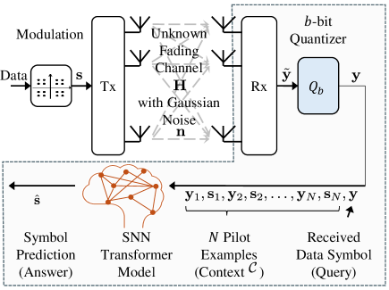
Figure 1: Illustration of in-context learning (ICL) for MIMO symbol detection.

Inspired by the neural architecture of human brains, which operate on as little as 20 Watts –, neuromorphic computing offers a compelling solution to these challenges [5]. Unlike the traditional artificial neural network (ANN) paradigm, neuromorphic computing relies on spiking neural networks (SNNs), which adopt a time-encoded, event-driven approach that closely resembles biological neural processing [6]. SNNs have been proven to offer energy savings for many workloads due to their sparse, multiplication-free, calculations [7].

Integrating SNNs into wireless communication systems offers a promising solution to the critical issue of energy consumption, and has been previously investigated for semantic communications [8, 9], integrated sensing and communications [10], and satellite communications [11].

As illustrated in Fig. 1, this paper evaluates a neuromorphic implementation of the transformer for ICL-based MIMO detection. This approach replaces ANNs with SNNs and implements the attention mechanism via stochastic computing [12], requiring no multiplications, but only logical AND operations and counting [13]. The proposed implementation is tested for MIMO detection in a link with a quantized receiver frontend. When using conventional digital CMOS hardware, the proposed implementation is shown to preserve accuracy, with a reduction in power consumption ranging from 5.4$\times$ to 26.8$\times$, depending on the model sizes, as compared to ANN-based implementations.

II Problem Formulation

As in [4], we consider a standard $N_{t}\times N_{r}$ MIMO link with $N_{t}$ transmit antennas, $N_{r}$ receive antennas, and a quantized front-end receiver. The transmitted data vector $\mathbf{s}$ consists of $N_{t}$ entries selected independently and uniformly from a constellation $\mathcal{S}$ with $K$ symbols. The average transmitting power is given by $\mathbb{E}[\mathbf{\|s\|}^{2}]=N_{t}$. The unknown fading channel is described by an $N_{r}\times N_{t}$ matrix $\mathbf{H}$, yielding the $N_{r}\times 1$ pre-quantization received signal vector

$$\tilde{\mathbf{y}}=\mathbf{H}\mathbf{s}+\mathbf{n},$$ (1)

with additive white complex Gaussian noise $\mathbf{n}$ having zero mean and unknown variance $\sigma^{2}$. Upon $b$-bit quantization, the received signal $\mathbf{y}$ available at the detector is written as

$$\mathbf{y}=Q_{b}(\tilde{\mathbf{y}}),$$ (2)

where the function $Q_{b}(\cdot)$ clips the received signal within a given range $[l_{\text{min}},l_{\text{max}}]$ and applies uniform quantization with a resolution of $b$ bits separately to the real and imaginary parts of each entry.

The objective of symbol detection is to estimate the transmitted data vector $\mathbf{s}$ from the corresponding received quantized signal vector $\mathbf{y}$. The detector does not know the channel and noise level $(\mathbf{H},\sigma^{2})$. Rather, it has access only to a context $\mathcal{C}$, which comprises of $N$ independent and identically distributed (i.i.d.) pilot receive-transmit pairs

$$\mathcal{C}=\{(\mathbf{s}_{i},\mathbf{y}_{i})\}^{N}_{i=1}$$ (3)

obtained from the channel model (1)-(2).

III In-Context Learning for MIMO Symbol Detection

Recently, ICL was proposed as a mechanism to estimate the symbol vector $\mathbf{s}$ for a new received signal $\mathbf{y}$ based on the context $\mathcal{C}$ in (3) [4]. Note that both the data input-output pair $(\mathbf{s},\mathbf{y})$ and the pilots in the context $\mathcal{C}$ are assumed to be generated i.i.d. from the model (1)-(2). As illustrated in Fig. 1, in this approach, a transformer model is fed the context $\mathcal{C}$ and the received signal $\mathbf{y}$ of interest and is trained to output an estimate $\hat{\mathbf{s}}$ of the transmitted signal vector $\mathbf{s}$.

Training is done by collecting a data set consisting of pairs of context $\mathcal{C}$ and transmitting data-received signal pair $(\mathbf{s},\mathbf{y})$. Each such data point is obtained for a given realization of the channel $\mathbf{H}$ and channel noise $\sigma^{2}$. Specifically, for each realization $(\mathbf{H},\sigma^{2})$, referred to as a task, $N_{\text{Example}}$ context-data pairs are generated and included in the data set (see Sec. II).

As shown in [4], and further discussed in Sec. VI, ICL can approach the performance of an ideal minimum mean squared error (MMSE) estimator that knows the statistics of channel $\mathbf{H}$, as well as the channel noise power $\sigma^{2}$. However, the implementation in [4] uses conventional ANN models, resulting in potentially prohibitive computing energy consumption levels. In this paper, we focus on evaluating the performance of a more efficient implementation of the transformer based on neuromorphic computing, i.e., on SNNs [13].

IV Preliminaries

This section introduces important background information for the definition of the considered SNN-based transformer.

IV-A Bernoulli Encoding and Stochastic Computing

Unlike ANNs, SNNs require the input data to be encoded in binary temporal sequences. In this work, Bernoulli encoding is adopted to convert a normalized real value $\overline{x}\in[0,1]$ into a discrete binary sequence of length $T$. This is done by assigning each encoded bit the value of ‘1’ independently with probability $\overline{x}$, and the value ‘0’ with probability $1-\overline{x}$, which is denoted as

$$x^{t}\sim\text{Bern}(\overline{x}),\;t=1,2,\ldots,T.$$ (4)

Bernoulli encoding enables the execution of stochastic computing [12].

In stochastic computing, the multiplication between two numbers $\overline{x}\in[0,1]$ and $\overline{y}\in[0,1]$ can be efficiently approximated by using the corresponding Bernoulli encoded sequences as

$$z^{t}=x^{t}\land y^{t},\;t=1,2,\ldots,T,$$ (5)

thus utilizing a simple logic AND gate $\land$. In fact, the probability of obtaining an output equal to 1 is equal to the desired product, i.e., $P(z^{t}=1)=\overline{x}\times\overline{y}$.

IV-B Leaky Integrate-and-Fire Neurons

In SNNs, neurons maintain an internal analog membrane potential and emit a spike when the potential crosses a threshold. A leaky integrate-and-fire (LIF) spiking neuron integrates incoming signals over discrete time steps. The membrane potential $V^{t}$ of an LIF neuron at time step $t$ evolves as

$$V^{t} =\beta V^{t-1}+I^{t},$$ (6)

where $\beta\in(0,1]$ represents the leak factor determining the rate of decay of the membrane potential over time, and $I^{t}$ is the input at time step $t$. When $V^{t}$ reaches or exceeds a threshold voltage $V_{\text{thresh}}$, the neuron fires a spike, i.e., $O^{t}=1$, resetting the potential $V^{t}$ to $0$. Otherwise, the neuron remains silent, producing $O^{t}=0$, i.e.,

$$\text{if }V^{t}\geq V_{\text{thresh}}\text{ then }\begin{cases}O^{t}=1,\\ V^{t}=0,\end{cases}\text{ else }O^{t}=0\text{ and \eqref{eq:V}}.$$ (7)

A layer of LIF neurons takes a binary vector $\mathbf{x}_{\text{in}}^{t}$, applies a linear transformation via a trainable weight matrix $\mathbf{W}$ and then applies the dynamics (7) separately to each output. Accordingly, the output of a LIF layer at time $t$ is denoted as

$$\mathbf{x}_{\text{out}}^{t}=\text{LIF}^{t}(\mathbf{W}\mathbf{x}_{\text{in}}^{t}),$$ (8)

The notation $\text{LIF}^{t}(\cdot)$ in (8) implicitly accounts for the dependence of the output $\mathbf{x}_{\text{out}}^{t}$ also on the past inputs through the membrane potentials (7) of the spiking neurons. Importantly, since the input signal $\mathbf{x}_{\text{in}}^{t}$ is binary, the matrix-vector multiplication $\mathbf{W}\mathbf{x}_{\text{in}}^{t}$ can be efficiently evaluated without the need to implement multiplications. This is one of the key reasons for the energy efficiency of SNNs as compared to ANNs.

V Spiking transformer for MIMO Symbol Detection

In this section, we detail the proposed implementation of MIMO symbol detection using a decoder-only spiking transformer. The proposed scheme, illustrated in Fig. 2, replaces the conventional ANN architecture adopted in [4], with a fully spiking neuron-based architecture that adopts a stochastic self-attention module [13].

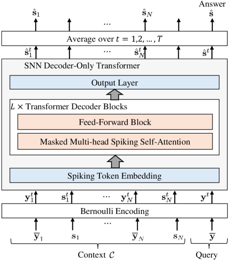
Figure 2: Block diagram of the proposed spiking transformer for ICL-based MIMO symbol detection.

V-A Normalization and Spike Encoding

The transformer model in Fig. 2 accepts the context $\mathcal{C}=\{\mathbf{y}_{1},\mathbf{s}_{1},\ldots,\mathbf{y}_{N},\mathbf{s}_{N}\}$ and received signal $\mathbf{y}$ as inputs, and produces an estimate $\hat{\mathbf{s}}$ of the transmitted symbol ${\mathbf{s}}$. To this end, first, the $N_{r}\times 1$ complex-valued received signal $\mathbf{y}$ is mapped to $2N_{r}\times 1$ real-valued vector $[\Re(\mathbf{y});\Im(\mathbf{y})]=\mathbf{y}^{\text{R}}$ by separating and concatenating real and imaginary parts, where $[\;\cdot\;;\;\cdot\;]$ denotes the operation of concatenating two column vectors. Each entry of vector $\mathbf{y}^{\text{R}}$ is normalized within the range $[0,1]$ as $\overline{\mathbf{y}}=(\mathbf{y}^{\text{R}}-l_{\text{min}}\mathbf{1})/(l_{\text{max}}-l_{\text{min}})$, where $\mathbf{1}$ is an all-ones vector, and we recall that $(l_{\text{max}},l_{\text{min}})$ is the dynamic range adopted by the quantizer $Q_{b}(\cdot)$ in (2). This procedure is also applied to the received pilot signal $\{\mathbf{y}_{i}\}_{i=1}^{N}$ in the context. Vectors $\mathbf{y}$, $\{\mathbf{y}_{i}\}_{i=1}^{N}$, and $\{\mathbf{s}_{i}\}_{i=1}^{N}$ are zero-padded as needed to obtain $D_{t}=\max(N_{t},2N_{r})\times 1$ vectors. The zero-padded sequences $\hat{\mathbf{y}}$, $\{\hat{\mathbf{y}}_{i}\}_{i=1}^{N}$, and $\{\mathbf{y}_{i}\}_{i=1}^{N}$ are then separately encoded into spiking signals via Bernoulli encoding (4), producing binary time sequences $\mathbf{y}^{t}$, $\{\mathbf{y}^{t}_{i}\}_{i=1}^{N}$, and $\{\mathbf{s}^{t}_{i}\}_{i=1}^{N}$, with $t=1,\cdots,T$, respectively.

V-B Spiking Token Embedding

Each $D_{t}\times 1$ vector in the set $\{\mathbf{y}^{t}_{1},\mathbf{s}^{t}_{1},\ldots,\mathbf{y}^{t}_{N},\mathbf{s}^{t}_{N},\mathbf{y}^{t}\}$ is considered a token. The spiking token embedding layer in Fig. 2 transforms each token into a vector of dimension $D_{e}\times 1$ using a LIF layer with a $D_{e}\times D_{t}$ trainable embedding matrix $\mathbf{W}_{e}$. This produces ${2N+1}$ embeddings as

$$\mathbf{E}_{0}^{t}=\text{LIF}^{t}([\mathbf{W}_{e}\mathbf{y}_{1}^{t};\;\mathbf{W}_{e}\mathbf{s}_{1}^{t};\;\ldots\;\mathbf{W}_{e}\mathbf{y}_{N}^{t};\;\mathbf{W}_{e}\mathbf{s}_{N}^{t};\;\mathbf{W}_{e}\mathbf{y}^{t}])$$ (9)

The resulting post-embedding sequence at time step $t$, $\mathbf{E}_{0}^{t}$, comprises $M=2N+1$ columns, each corresponding to an embedded token with $D_{e}$ binary entries.

V-C Transformer Decoder Layers

The spike embedding $\mathbf{E}_{0}^{t}$ undergoes processing through $L$ successive transformer decoder layers. Each $l$-th layer, with $l=1,\ldots,L$, accepts the $D_{e}\times M$ binary output $\mathbf{E}_{l-1}^{t}$ from the previous layer as input, and outputs a $D_{e}\times M$ binary matrix $\mathbf{E}_{l}^{t}$. The first sub-layer implements a masked multi-head spiking self-attention mechanism, whereas the subsequent sub-layer consists of a two-layer fully connected feed-forward network. Residual connections are utilized around each sub-layer, followed by layer normalization and a LIF neuron model.

V-C1 Masked Multi-Head Spiking Self-Attention Mechanism

The first sub-layer deploys $n_{h}$ attention “heads”. For the $h$-th head, the input $\mathbf{E}^{t}_{l-1}$ is transformed into query $\mathbf{Q}_{h}^{t}$, key $\mathbf{K}_{h}^{t}$, and value $\mathbf{V}_{h}^{t}$ matrices by applying separate encoding LIF layers as $\mathbf{Q}_{h}^{t}=\text{LIF}^{t}(\mathbf{W}_{Q}\mathbf{E}^{t}_{l-1})$, $\mathbf{K}_{h}^{t}=\text{LIF}^{t}(\mathbf{W}_{K}\mathbf{E}^{t}_{l-1})$, and $\mathbf{V}_{h}^{t}=\text{LIF}^{t}(\mathbf{W}_{V}\mathbf{E}^{t}_{l-1})$, where $\mathbf{W}_{Q}$, $\mathbf{W}_{K}$, and $\mathbf{W}_{V}$ represent trainable $D_{K}\times D_{e}$ real-valued weight matrices, with $D_{K}=D_{e}/n_{h}$ assumed to be an integer. Subsequently, dot-product attention is executed through a specially designed architecture termed masked stochastic spiking attention (MSSA) [13], as detailed in Algorithm 1.

Algorithm 1 Masked Stochastic Spiking Attention (MSSA)

1:Input: $D_{K}\times M$ binary matrix sequences $\mathbf{Q}^{t},\mathbf{K}^{t},\mathbf{V}^{t}$ for $t=1,\ldots,T$, dimension $D_{K}$ (corresponding to one head $h$)

2:Output: $D_{K}\times M$ binary matrix sequence $\mathbf{F}^{t}$ for $t=1,\ldots,T$ (corresponding to one head $h$)

3:for $t=1$ to $T$ do

4:     for each $(m,m^{\prime})$ in $M\times M$ do

5:         Compute the query-key dot product for the $(m,m^{\prime})$-th entry of the attention matrix:  

6:         if $m\leq m^{\prime}$ then

7:              $\tilde{A}^{t}_{m,m^{\prime}}=\sum_{d=1}^{D_{K}}Q^{t}_{d,m}\land K^{t}_{d,m^{\prime}}$

8:         else

9:              $\tilde{A}^{t}_{m,m^{\prime}}=0$ (casual mask)

10:         end if

11:         Normalize and encode $\tilde{A}^{t}_{m,m^{\prime}}$ to obtain the binary attention parameter $A^{t}_{m,m^{\prime}}$:

12:          $A^{t}_{m,m^{\prime}}\sim\mathrm{Bern}\left(\frac{1}{D_{K}}\tilde{A}^{t}_{m,m^{\prime}}\right)$

13:     end for

14:     for each $(d,m)$ in $D_{K}\times M$ do

15:         Compute the $d$-th entry of each $m$-th output token as

16:          $\tilde{F}_{d,m}=\sum_{m^{\prime}=1}^{M}A^{t}_{m,m^{\prime}}\land V^{t}_{d,m^{\prime}}$

17:         Normalize and encode $\tilde{F}_{d,m}$ to obtain $F^{t}_{d,m}$ as

18:          $F^{t}_{d,m}\sim\mathrm{Bern}\left(\frac{1}{M}\tilde{F}_{d,m}\right)$

19:     end for

20:end for

The deployment of MSSA leverages the binary nature of the inputs, enabling the efficient realization of the dot-product attention mechanism using simple logic AND gates and counters in lines 7 and 16 in Algorithm 1. This circumvents the need for computationally expensive multiplication units. A potential hardware implementation of MSSA can be achieved by modifying the approach described in [13].

By Algorithm 1, the output of the first sub-layer is obtained by the column-wise concatenation of the outputs from each head $h$, obtaining the binary $D_{e}\times M$ matrix

$$\mathbf{G}^{t}=\left[\mathbf{F}_{1}^{t}\;;\;\mathbf{F}_{2}^{t}\;;\;\ldots\;;\;\mathbf{F}_{n_{h}}^{t}\right].$$ (10)

V-C2 Feed-Forward Network

The feed-forward network applies two sequential LIF layers, as described by

$$\mathbf{E}^{t}_{l}=\text{LIF}^{t}(\mathbf{W}_{2}\text{LIF}^{t}(\mathbf{W}_{1}\mathbf{G}^{t})),$$ (11)

where the trainable real-valued matrices $\mathbf{W}_{1}$ and $\mathbf{W}_{2}$ are of dimensions $D_{h}\times D_{e}$ and $D_{e}\times D_{h}$, respectively. The output $\mathbf{E}^{t}_{l}$ constitutes the output of the $l$-th transformer decoder layer.

V-D Output Layer and Accumulation

The output layer consists of a linear transformation that projects the embedding dimension into the number of classes $K^{N_{t}}$ via a trainable real-valued $K^{N_{t}}\times D_{e}$ matrix $\mathbf{W}_{O}$ as $\mathbf{O}^{t}=\mathbf{W}_{O}\mathbf{E}^{t}_{L}$. The outputs across time steps are accumulated and averaged to produce the final $K^{N_{t}}\times(2N+1)$ output $\mathbf{O}$:

$$\mathbf{O}=\frac{1}{T}\sum_{t=1}^{T}\mathbf{O}^{t}=[\mathbf{o}_{1}\;\mathbf{o}_{2}\;\ldots\;\mathbf{o}_{2N+1}].$$ (12)

The network’s output is represented by the last token, $\hat{\mathbf{s}}=\mathbf{o}_{2N+1}$, with the index of the largest element being the symbol prediction.

V-E Off-Line Pre-Training

For off-line pre-training, we assume the availability of a dataset with $N_{\text{Train}}$ pairs of fading channel coefficients and noise variance, $\{(\mathbf{H}_{n},\sigma^{2}_{n})\}_{n=1}^{N_{\text{Train}}}$, which are sampled i.i.d.. For each pre-training task, we are provided $N_{\text{Example}}$ pairs of context $\mathcal{C}$ and test input-output $\{\mathbf{y},\mathbf{s}\}$. The objective of pre-training is to minimize the cross-entropy loss averaged over all training tasks with respect to the model parameters $\theta$. The training loss function is accordingly defined as

$$L(\theta)=\sum_{n=1}^{N_{\text{Train}}}\sum_{l=1}^{N_{\text{Example}}}\left[-\sum_{c=1}^{K^{N_{t}}}f(\mathbf{s}_{n})[c]\log\left(\hat{\mathbf{s}}[c]\right)\right],$$ (13)

where $f(\cdot)$ denotes the one-hot encoding function that converts $\mathbf{s}_{n}$ into a binary one-hot vector of length $K^{N_{t}}$, and the notation $[c]$ signifies the selection of the $c$-th element.

VI Experimental Results and Conclusions

This section evaluates the effectiveness of our SNN-based transformer architecture for MIMO symbol detection. We compare the performance and energy efficiency of the SNN-based implementation with an established benchmark algorithm, as well as a baseline ANN-based implementation of the ICL detector proposed in [4].

VI-A Experimental Setup

We investigate a MIMO system configuration featuring $N_{t}=N_{r}=2$ antennas. We set $K=4$, so that the channel input utilizes a QPSK modulation scheme. A mid-tread uniform 4-bit quantizer, with clipping boundaries at $l_{\text{min}}=-4$ and $l_{\text{max}}=4$, quantizes the received signal as (2). The channel matrix elements adhere to an i.i.d. complex Gaussian distribution $\mathcal{CN}(0,1)$, and the signal-to-noise ratio (SNR) is uniformly sampled in the range of $[0,30]$ dB.

The proposed symbol detection model utilizes an SNN transformer characterized by an embedding dimension $D_{e}=256$, a total of $L=4$ decoder layers, and $n_{h}=8$ attention heads. The model undergoes training on a pre-training dataset comprising of $N_{\text{Train}}=2^{15}=32768$ combinations of tasks $(\mathbf{H}_{n},\sigma^{2}_{n})$. The context $\mathcal{C}$ includes $N=20$ examples.

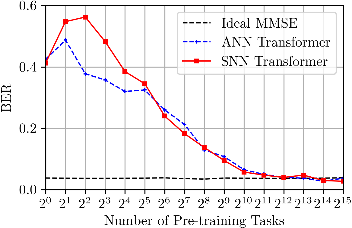
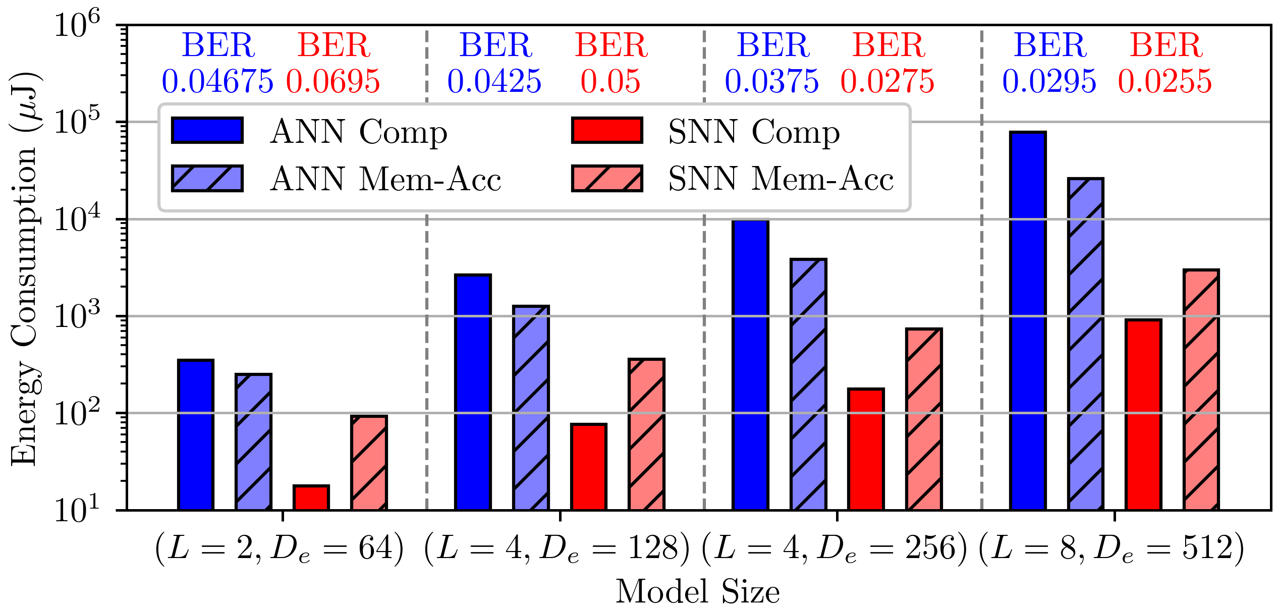
Figure 3: (a) Detection BER for ANN and SNN transformers, pre-trained with varying numbers of tasks and tested under an SNR of 10 dB. Both models use $L=4$ layers, $n_{h}=8$ heads, and an embedding dimension of $D_{e}=256$. (b) Computing energy consumption and memory access energy consumption for ANN and SNN transformers of varying sizes, marked with the lowest BER achievable with a pre-training size of $N_{\text{Train}}=32768$. For the SNN model, the number of timesteps is set to $T=4$ for both panels.

The baselines include 1) Ideal MMSE: The MMSE equalizer with knowledge distribution of the testing channel $\mathbf{H}$ and noise variance $\sigma^{2}$; and 2) ANN transformer: the ANN counterpart of the proposed SNN transformer which follows the architecture as [4] and shares the same size parameters as the SNN.

VI-B Performance Test of ICL-based Symbol Detection

We first study the generalization performance of the ICL-based symbol detector as a function of the number of pre-training tasks $N_{\text{Train}}$. Fig. 3 presents the bit error rate (BER) for our SNN-based symbol detector as compared to its ANN-based counterpart. The BER is evaluated across a range of pre-training tasks, exponentially increasing from $2^{0}$ to $2^{15}$. The SNN transformer demonstrates performance comparable with the ANN transformer when the number of training tasks is sufficiently large, i.e., when $N_{\text{Train}}\geq 2^{5}$. Both implementations gradually approach the performance of the ideal MMSE equalizer.

VI-C Energy Efficiency

We now estimate the energy consumption associated with the execution of ICL inference for the SNN-based symbol detector and its ANN-based counterpart. This estimation accounts for all necessary computational and memory access operations, both read and write, as per the methodology presented in [14]. In addition to the network size $(L,D_{e})=(4,256)$, we examine the configurations $(2,64)$, $(4,128)$, and $(8,512)$ to evaluate the tradeoffs between performance and energy usage. The number of SNN time steps is set to $T=4$. For both ANNs and SNNs, model parameters and pre-activations are quantized using an 8-bit integer (INT8) format. The energy consumption calculations are based on the standard energy metrics for 45 nm CMOS technology reported in [15, 16]. We assume that the required data for computations are stored in the on-chip static random-access memory (SRAM), with a cache that is sufficiently sized to hold all model parameters, thus allowing for each parameter to be read a single time during the inference process.

Fig. 3 shows the energy consumption evaluated for ANN- and SNN-based implementations with different model sizes. The energy consumption is broken down into separate contributions for computational processes and for memory access. Each model size and implementation is marked with the BER attained at an SNR of 10 dB. We observe that the SNN-based implementation of size ($L=2$, $D_{e}=64$), exhibits a $20\times$ improvement in computational energy cost and $2.6\times$ saving in memory access cost as compared to its ANN-based counterpart, while achieving a worse BER, namely 0.070 against 0.047 for the ANN-based implementation. When increasing the model size to ($L=8$, $D_{e}=512$), the SNN-based detector significantly outperforms the ANN-based implementation with an $86\times$ reduction in computation energy and an $8.7\times$ reduction in memory access energy as compared to its ANN-based counterpart, while also achieving slightly better BER, namely 0.026 against 0.030.

References

- [1] X. You, C.-X. Wang, J. Huang, X. Gao, Z. Zhang, M. Wang, Y. Huang, C. Zhang, Y. Jiang, J. Wang et al., “Towards 6G wireless communication networks: Vision, enabling technologies, and new paradigm shifts,” Science China Information Sciences, vol. 64, pp. 1–74, 2021.
- [2] S. Garg, D. Tsipras, P. S. Liang, and G. Valiant, “What can transformers learn in-context? a case study of simple function classes,” Advances in Neural Information Processing Systems, vol. 35, pp. 30 583–30 598, 2022.
- [3] V. Rajagopalan, V. T. Kunde, C. S. K. Valmeekam, K. Narayanan, S. Shakkottai, D. Kalathil, and J.-F. Chamberland, “Transformers are efficient in-context estimators for wireless communication,” arXiv preprint arXiv:2311.00226, 2023.
- [4] M. Zecchin, K. Yu, and O. Simeone, “In-context learning for mimo equalization using transformer-based sequence models,” arXiv preprint arXiv:2311.06101, 2023.
- [5] C. Mead, “Neuromorphic electronic systems,” Proceedings of the IEEE, vol. 78, no. 10, pp. 1629–1636, 1990.
- [6] A. Tavanaei, M. Ghodrati, S. R. Kheradpisheh, T. Masquelier, and A. Maida, “Deep learning in spiking neural networks,” Neural networks, vol. 111, pp. 47–63, 2019.
- [7] M. Davies, A. Wild, G. Orchard, Y. Sandamirskaya, G. A. F. Guerra, P. Joshi, P. Plank, and S. R. Risbud, “Advancing neuromorphic computing with loihi: A survey of results and outlook,” Proceedings of the IEEE, vol. 109, no. 5, pp. 911–934, 2021.
- [8] N. Skatchkovsky, H. Jang, and O. Simeone, “Spiking neural networks—part iii: Neuromorphic communications,” IEEE Communications Letters, vol. 25, no. 6, pp. 1746–1750, 2021.
- [9] J. Chen, N. Skatchkovsky, and O. Simeone, “Neuromorphic integrated sensing and communications,” IEEE Wireless Communications Letters, vol. 12, no. 3, pp. 476–480, 2022.
- [10] ——, “Neuromorphic wireless cognition: Event-driven semantic communications for remote inference,” IEEE Transactions on Cognitive Communications and Networking, vol. 9, no. 2, pp. 252–265, 2023.
- [11] F. Ortiz, N. Skatchkovsky, E. Lagunas, W. A. Martins, G. Eappen, S. Daoud, O. Simeone, B. Rajendran, and S. Chatzinotas, “Energy-efficient on-board radio resource management for satellite communications via neuromorphic computing,” IEEE Transactions on Machine Learning in Communications and Networking, 2024.
- [12] B. R. Gaines, “Stochastic computing systems,” Advances in Information Systems Science: Volume 2, pp. 37–172, 1969.
- [13] Z. Song, P. Katti, O. Simeone, and B. Rajendran, “Stochastic spiking attention: Accelerating attention with stochastic computing in spiking networks,” arXiv preprint arXiv:2402.09109, 2024.
- [14] G. Datta, S. Kundu, A. R. Jaiswal, and P. A. Beerel, “ACE-SNN: Algorithm-Hardware Co-design of Energy-Efficient & Low-Latency Deep Spiking Neural Networks for 3D Image Recognition,” Frontiers in Neuroscience, vol. 16, 2022.
- [15] A. Pedram, S. Richardson, M. Horowitz, S. Galal, and S. Kvatinsky, “Dark Memory and Accelerator-Rich System Optimization in the Dark Silicon Era,” IEEE Design & Test, vol. 34, no. 2, pp. 39–50, 2017.
- [16] C. Buffa, L. Hernandez-Corporales, C. A. P. Cruz, A. Q. Alonso, and A. Wiesbauer, “Voltage controlled oscillator based analog-to-digital converter including a maximum length sequence generator,” Jan. 5 2021, US Patent 10,886,930.