Constraining electron number density in the Sun via Earth-based neutrino flavor data

Abstract

Neutrino flavor transformation offers a window into the physics of various astrophysical environments, including our Sun and the more exotic environs of core-collapse supernovae and binary neutron-star mergers. Here, we apply an inference framework – specifically: statistical data assimilation (SDA) – to neutrino flavor evolution in the Sun. We take a model for solar neutrino flavor evolution, together with Earth-based neutrino measurements, to infer solar properties. Specifically, we ask what signature of the radially-varying solar electron number density $n_{e}(r)$ is contained within these Earth-based measurements. Currently, the best estimates of $n_{e}(r)$ come from the standard solar model. We seek to ascertain, through novel application of the SDA method, whether estimates of the same from neutrino data can serve as independent constraints.

I.   INTRODUCTION

Neutrinos are ubiquitous in astrophysical settings, and in certain environments they significantly shape the physics. In a core-collapse supernova (CCSN) and neutron star mergers, abundant neutrino emission is the cooling mechanism of the resulting compact object. These environments are dense enough that a non-negligible fraction of the neutrinos can absorb or re-scatter as they make their way through the surrounding medium. This has significant implications for energy transport and heavy element synthesis. For this reason, neutrino observations could offer insight into the interiors and collapse mechanisms of these objects, as well as properties of the neutrinos themselves. In particular, neutrino "flavor," a property that defines the manner in which neutrinos interact with other matter particles, assumes profound importance Balantekin et al. (1988); Fuller et al. (1992); Qian et al. (1993); Fuller (1993); Fuller and Meyer (1995); Balantekin (1999); Duan et al. (2011); Wu et al. (2015, 2016); Sasaki et al. (2017); Balantekin (2018a, b); Xiong et al. (2019, 2020).

The high density of neutrinos in supernova and merger environments is such that neutrino-neutrino interactions introduce nonlinear elements in their flavor evolution and transport. Powerful numerical integration codes exist for obtaining solutions to the flavor evolution problem in these compact object environments Duan et al. (2006, 2008); Richers et al. (2019, 2021a, 2021b); Kato et al. (2021); Nagakura (2022); George et al. (2022). They require, however, adopting certain physical assumptions regarding the symmetries of the problem, and in recent years it has been shown that relaxing these assumptions reveals physics that had been hidden by them (e.g., see Ref. Tamborra and Shalgar (2021); Richers and Sen (2022); Patwardhan et al. (2023); Balantekin et al. (2023) and references therein).

In previous papers Armstrong et al. (2022); Armstrong (2022); Armstrong et al. (2017, 2020); Rrapaj et al. (2021), we applied an inference technique – a fundamentally different framework compared to forward integration – to examine nonlinear collective oscillations in core-collapse supernovae, using simulated data. Inference is a means to optimize a model given measurements, where measurements are assumed to arise from model dynamics. The specific technique used is statistical data assimilation (SDA), which was invented for the case of sparse data in numerical weather prediction Kimura (2002); Kalnay (2003); Evensen (2009); Betts (2010); Whartenby et al. (2013); An et al. (2017), and since then in neurobiology Schiff (2009); Toth et al. (2011); Kostuk et al. (2012); Hamilton et al. (2013); Meliza et al. (2014); Nogaret et al. (2016); Armstrong (2020).

Following our simulated experiments with CCSN, we next gave the SDA procedure the critical challenge of handling real neutrino data. For this task we moved to a solar model. Solar neutrino data are copious, while CCSN neutrinos are limited to one event: SN1987A Hirata et al. (1987); Bionta et al. (1987); Alekseev et al. (1987). In addition, the solar neutrino problem does not have the underlying nonlinearity of the supernova neutrino problem. In the Sun, neutrinos emerge from the nuclear reactions that provide the energy flux and pressure to support the star against its gravity. The neutrinos can efficiently transport a part of the energy released in nuclear reactions away from the core of the sun, but due to the low matter density, these neutrinos do not undergo scattering/absorption to any significant extent. Neutrino observations could, however, provide independent estimates of poorly constrained solar properties.

In our first application of SDA to a solar model (Ref. Laber-Smith et al. (2023)), the SDA procedure successfully reconciled Earth-based neutrino measurements Agostini et al. (2018); Aharmim et al. (2010) with the model, for the case wherein all solar parameters were taken to be known. Now we take a step further: we ask what information Earth-based neutrino flavor measurements contain about the radially-varying solar electron number density $n_{e}(r)$.

Standard simulations of solar neutrino spectra take $n_{e}(r)$ as input, where $n_{e}(r)$ has been calculated by the standard solar model, given observed surface abundances. There, the simulation is framed as an initial-value-problem (IVP). We, on the other hand, seek to estimate solar properties directly from neutrino data – using a two-point boundary-value-problem (BVP) formulation. Using the SDA method together with the neutrino data would be a novel way to estimate $n_{e}(r)$. We should point out that although applying the SDA method to this problem is a new approach, the idea of estimating solar density through neutrino observations itself has been considered before using other approaches Balantekin et al. (1998); Lopes and Turck-Chièze (2013). With that in mind, in this paper we take Earth-based electron-flavor survival probabilities Agostini et al. (2018) together with an adiabatic model of flavor evolution assumed to underlie those data, to determine (i) the electron density $n_{e}$ at the solar center, and (ii) whether the data show preference for a particular analytical form for the full trajectory $n_{e}(r)$.

II.   INPUT

A.   Model of neutrino flavor evolution

To model the flavor evolution of neutrinos inside the Sun, we follow the same framework as Laber-Smith et al. (2023). We consider mixing between $\nu_{e}$ and $\nu_{x}$ (a superposition of $\nu_{\mu}$ and $\nu_{\tau}$) in a two-flavor framework with a mixing angle $\theta\simeq\theta_{12}$ and $\theta_{13}\simeq 0$. All neutrinos are assumed to be produced in the center of the Sun in purely $\nu_{e}$ flavor states, and subsequently, they experience flavor evolution through a combination of vacuum oscillations and matter effects inside the Sun. Sufficiently energetic neutrinos undergo a mass-level crossing, i.e., the Mikheyev-Smirnov-Wolfenstein (MSW) resonance, and consequently experience enhanced coherent $\nu_{e}$-$\nu_{x}$ transformations as they pass through the solar envelope.

The neutrinos may be represented using a polarization vector (i.e., a Bloch vector) with real-valued components, which are related to the wavefunction amplitudes $\psi_{e}=\innerproduct{\nu_{e}}{\psi}$ and $\psi_{x}=\innerproduct{\nu_{x}}{\psi}$ in the following manner:

$$\vec{P}=\left(\begin{array}[]{c}P_{x}\\ P_{y}\\ P_{z}\end{array}\right)=\left(\begin{array}[]{c}\psi_{e}\psi_{x}^{*}+\psi_{e}^{*}\psi_{x}\\ i(\psi_{e}\psi_{x}^{*}-\psi_{e}^{*}\psi_{x})\\ |\psi_{e}|^{2}-|\psi_{x}|^{2}\\ \end{array}\right).$$ (1)

In particular, the $\hat{z}$ component $P_{z}$ of the neutrino polarization vector denotes the net flavor content of that particular neutrino ($e$-flavor minus $x$-flavor), and is related to the electron-flavor survival probability $P_{ee}$ as $P_{z}=2P_{ee}-1$. Since the neutrinos are assumed to be produced as pure $\nu_{e}$ states in the center of the Sun, we have the initial condition $P_{z}=1$ and $P_{x}=P_{y}=0$ for each neutrino. The dynamical equation for neutrino flavor evolution, when expressed in this language, assumes the form of a spin-precession equation:

$$\diff{\vec{P}}{r}=\left(\omega\vec{B}+V(r)\hat{z}\right)\times\vec{P},$$ (2)

The external field driving this precession in flavor space consists of a “vacuum” part $\omega\vec{B}$, and a “matter” part $\vec{V}=V(r)\hat{z}$. $\omega=\delta m^{2}/(2E)$ is the vacuum oscillation frequency of a neutrino with energy $E$ and mass-squared difference $\delta m^{2}$. The unit vector $\vec{B}=\sin(2\theta)\hat{x}-\cos(2\theta)\hat{z}$ points along the direction of the $\ket{\nu_{2}}$ mass eigenstate in flavor space. The function $V(r)$ is proportional to the electron number density, as described in Sec. B. A neutrino propagating out through the Sun encounters a mass-level crossing (MSW resonance) when $V(r)-\omega\cos{2\theta}=0$, i.e., when the $\hat{z}$ component of the external field vanishes.

We take our domain of state-variable evolution to span from the center of the Sun to a radius of ${R_{\odot}}/{2}$ (half the solar radius), where the matter density is sufficiently low to be considered in the vacuum regime (i.e., $V(r)\ll\omega\cos{2\theta}$). To connect the state variable evolution within the Sun to measurements of neutrino flavor at the earth, however, requires some careful consideration. One has to take into account that the neutrinos kinematically decohere as they propagate over sufficiently long distances, i.e., the $\nu_{1}$ and $\nu_{2}$ mass eigenstates become separated in space as they are moving at slightly different speeds. As a result, the detector “catches” only one mass eigenstate at a time, and not a coherent superposition of both. Taking this effect into account leads to the following transformation between the polarization vector components at $r_{\text{final}}=R_{\odot}/2$ – the outer endpoint of our domain, and the neutrino electron-flavor survival probability measured on Earth, $P_{ee,\oplus}$ Laber-Smith et al. (2023); Dighe et al. (1999):

$$\left(1-\sin^{2}2\theta\right)P_{z,\text{final}}-\cos 2\theta\sin 2\theta P_{x,\text{final}}=2P_{ee,\oplus}-1.$$ (3)

B.   Model for electron number density $n_{e}$

The matter potential $V(r)$ of Eq. 2 is related to the electron number density $n_{e}$ as:

$$V(r)=\sqrt{2}G_{F}n_{e}\left(r\right).$$

This term embodies the neutrino mass Wolfenstein correction Wolfenstein (1978): it arises from neutrino coherent forward scattering on the background electrons.

We chose two distinct forms for the matter potential, to check for invariance of results across the two. Our motivation was as follows. If the change in $V(r)$ is slow enough to allow for adiabatic evolution, the resulting neutrino state would depend solely on the matter potential at the endpoints, $V_{0}$ and $V_{f}$, and not strongly on the shape of $V(r)$ itself. In choosing two versions for $V(r)$, we aimed to test this expectation.

The first version for $V(r)$ was an exponential decay:

$$V(r)=V_{0}\exp{-\frac{2r}{R_{\odot}}\ln\frac{V_{0}}{V_{f}}}.$$ (4)

This form can approximate the decay of the matter profile of the standard solar model near the edge of the Sun, while remaining analytically simple.

The second version was a logistic function:

$$V(r)=V_{0}\left[\frac{\left(e^{k\frac{R_{\odot}}{2}}-1\right)\left(\frac{V_{f}}{V_{0}}\right)^{q}}{\left(e^{k\frac{R_{\odot}}{2}}-e^{kr}\right)\left(\frac{V_{f}}{V_{0}}\right)^{q}-1+e^{kr}}\right]^{1/q}$$ (5)

Here, $q=1.7$ and $k=1.35\times 10^{-5}\text{ km}^{-1}$. We adopted this form so that, together with the chosen parameter values, it would more closely match the shape of the matter potential from the standard solar model, compared to the simpler exponential form. Namely, the falloff near the solar center is shallower.

Both models were designed so that altering the value of $V_{0}$ would keep $V\left({R_{\odot}}/{2}\right)=V_{f}$ fixed, at a value near zero, in agreement with the standard solar model Bahcall et al. (2005). The aim of this paper, to be described in Sec. IV, was to estimate from data the value of $V_{0}$ – the matter potential at the solar center. (Model quantities taken to be known are listed in Table 1.)

Table 1: Model quantities taken to be known. The $V_{0}$ values here refer to the initial (proof-of-concept) stage of testing the procedure, prior to parameter estimation (see Sec. IV).

Parameter	Value [unit]
$R_{\odot}$	$6.957\times 10^{5}\text{ km}$
$\theta$	0.5838 rad
$G_{F}$	$1.166\times 10^{-11}\text{ MeV}^{-2}$
$\delta m^{2}$	$7.53\times 10^{-17}\text{ MeV}^{2}$
$V_{0}$ values	$0.015,0.02,0.025,0.03,0.035,$ $0.055,0.075,0.095\text{ km}^{-1}$

C.   Data

We used ⁸B day-time neutrino flux observed by the Borexino Agostini et al. (2018) experiment. We used only the observed pp-chain neutrinos (specifically, ⁸B neutrinos), and not the carbon-nitrogen-oxygen cycle (CNO) neutrinos. This is a reasonable choice for the Sun: its core temperature is relatively low, so that few CNO neutrinos are produced. In addition, for simplicity we used day-time data only. The Borexino survival probabilities are listed in Table 2.

Table 2: Energy bins and corresponding survival probabilities $P_{ee,i}$ from the Borexino experiment Agostini et al. (2018). These energy values were also adopted for the model.

Parameter	Energy [MeV]	Parameter	Probability
$E_{1}$	7.4	$P_{ee,1}$	$0.39\pm 0.09$
$E_{2}$	8.1	$P_{ee,2}$	$0.37\pm 0.08$
$E_{3}$	9.7	$P_{ee,3}$	$0.35\pm 0.09$

III.   THE INFERENCE METHOD

This section offers a brief description of our methodology. For details, we refer the reader to Ref. Laber-Smith et al. (2023).

A.   General formulation of SDA

SDA assumes that any observed quantities arise from an underlying dynamical model, and that those quantities represent only a sparse subset of the model’s full degrees of freedom. We call this model $F_{a}(\bm{x}(r),\bm{p}(r))$; $a=1,2,\ldots,D$: a set of $D$ ordinary differential equations governing the evolution of $D$ state variables $x_{a}(r)$, where $r$ is our parameterization and $\bm{p}$ are unknown parameters ($p$ in number).

A subset $L$ of the $D$ state variables can be associated with measured quantities. We seek to estimate the evolution of all $D$ state variables that is consistent with those $L$ measurements, and to predict their evolution at locations where measurements have not been obtained.

B.   A path integral approach

We can cast SDA as a path integral formulation, in the following sense. We seek the probability of obtaining a path $\bm{X}$ given observations $\bm{Y}$:

$$P(\bm{X}|\bm{Y})=e^{-A_{0}(\bm{X},\bm{Y})},$$

which becomes a problem of minimizing the quantity $A_{0}$, our "action." Further, we use an optimization formulation, where the cost function of the optimizer is equivalent to the action on a path in the state space. The cost function surface is $((D+p)\times(N+1))$-dimensional, where $N+1$ is the number of discrete model locations, which we take to be independent dimensions. We seek the path $\bm{X}^{0}=\{\bm{x}(0),\ldots,\bm{x}(N),\bm{p}(0),\ldots,\bm{p}(N)\}$ in state space that corresponds to the lowest cost. We find minima via the variational method Oden and Reddy (2012).

After many simplifications, $A_{0}$ can be written in the following computationally implementable form:

$$\begin{split}A_{0}=&R_{f}A_{\text{model}}+R_{m}A_{\text{meas}}\\ A_{\text{model}}=&\frac{1}{{N}D}{\sum}_{n\in\{\text{odd}\}}^{N-2}\,{\sum}_{a=1}^{D}\\ &\Bigg{[}\left\{x_{a}(r_{n+2})-x_{a}(r_{n})-\frac{\delta r}{6}[F_{a}(\bm{x}(r_{n}),\bm{p}(r_{n}))+4F_{a}(\bm{x}(r_{n+1}),\bm{p}(r_{n+1}))+F_{a}(\bm{x}(r_{n+2}),\bm{p}(r_{n+2}))]\right\}^{2}\\ &+\left\{x_{a}(r_{n+1})-\frac{1}{2}\left(x_{a}(r_{n})+x_{a}(r_{n+2})\right)-\frac{\delta r}{8}[F_{a}(\bm{x}(r_{n}),\bm{p}(r_{n}))-F_{a}(\bm{x}(r_{n+2}),\bm{p}(r_{n+2)})]\right\}^{2}\Bigg{]}\\ A_{\text{meas}}=&\frac{1}{N_{\text{meas}}}{\sum}_{r_{m}\in\{\text{meas}\}}\,{\sum}_{l=1}^{L}\left[\left(y_{l}\left(r_{m}\right)-h_{l,m}(\bm{x}(r_{m})\right)^{2}\right]\end{split}$$ (6)

In $A_{\text{model}}$, adherence to the model evolution is required of all $D$ state variables $x_{a}$. The outer sum on $n$ runs through all odd-numbered discretized locations. The inner sum on $a$ runs through all $D$ state variables. The terms within the first and second sets of curly brackets represent the errors in the first and second derivatives, respectively, of the state variables.

In $A_{\text{meas}}$, we require adherence to the measurements of any measured quantities. The variables $y_{l}$, for $l=1,\ldots,L$, are the $L$ components that are measured at locations $r_{m}\in\{{\text{meas}}\}$; the number of locations is $N_{\text{meas}}$. We will compare these values to the components $h_{l,m}(\bm{x})$. These $h_{l,m}$ are transfer functions translating the model state variables to the measured quantities. Here, the measured quantities are the values of $P_{z}$ of each neutrino, at two locations: the center of the Sun, and the surface of Earth (the "measurement" at the center of the Sun is really a robust theoretical expectation on neutrino flavor). At the Sun’s center, we can compare the measurement directly to the model’s $P_{z}$, rendering the transfer functions trivial (that is: $h_{0}(\vec{P})=P_{z}$.) The translation at the surface of Earth, however, is more involved. This is because our model grid does not extend beyond the Sun (i.e., beyond $r_{\text{final}}=R_{\odot}/2$), and the neutrinos experience kinematic decoherence on their way to Earth (see Sec. A and Ref. Laber-Smith et al. (2023) for an explanation). We connect model to measurement at this end by comparing the $P_{z}$ measurement at Earth to an extrapolated $P_{z}$ value derived from the Polarization vector components at $R_{\odot}/2$ [as given by Eq. (3)]. In this way, there is an equivalency between measuring $P_{z}$ at Earth and measuring a linear combination of $P_{z}$ and $P_{x}$ at $R_{\odot}/2$. Thus, the transfer function at this end is:

$$h_{\text{final}}(\vec{P})=\left(1-\sin^{2}2\theta\right)P_{z}-\cos 2\theta\sin 2\theta\,P_{x},$$ (7)

for each neutrino energy. Then the measurement term becomes:

$$\begin{split}A_{\text{meas}}=&\frac{1}{N_{\text{meas}}}\sum_{k=1}^{N_{\nu}}\left[\left(P_{z,k}^{\text{meas}}\left(0\right)-P_{z,k}\left(0\right)\right)^{2}+\left(P_{z,k}^{\text{meas}}(\oplus)-h_{\text{final}}\left(\vec{P}_{k}\left(\frac{R_{\odot}}{2}\right)\right)\right)^{2}\right].\end{split}$$ (8)

Here, the subscript $k=\{1,\ldots,N_{\nu}\}$ indexes the neutrino energy bins. $P_{z,k}^{\text{meas}}$ is the measurement of $P_{z}$ at the specified location (with $0$ being the center of the sun, and $\oplus$ being the Earth).

C.   Multiple solutions

The action surface for a nonlinear model will be non-convex, and our search algorithm is descent-only. Thus we face the problem of multiple minima. To identify a lowest minimum, we iteratively anneal Ye et al. (2015) in terms of the coefficients $R_{f}$ and $R_{m}$ of the model and measurement error terms, respectively, of Eq. (6).

We set $R_{m}$ to 1.0, and write $R_{f}$ as $R_{f,0}\alpha^{\beta}$. The values of $R_{f,0}$ and $\alpha$ are chosen to work best for the particular model at hand (in this paper, they are $10^{3}$ and $2.0$, respectively), and $\beta$ is the annealing parameter, initialized at 1. The first annealing iteration takes the measurement error to dominate: with the model dynamics imposed relatively weakly, the action surface is rather smooth, and we obtain an estimate of $A_{0}$. The second iteration involves an integer increment in $\beta$, which places faint structure upon the action surface, and the search begins anew from the initial estimate of $A_{0}$. We anneal toward the deterministic limit where $R_{f}\gg R_{m}$, aiming to remain sufficiently close to the lowest minimum along the way.

IV.   SPECIFIC INFERENCE TASK

Our model contained neutrinos with three distinct energies, chosen to replicate the Borexino experiment’s three energy bins. For each neutrino energy, the flavor evolution was constrained by two measurements. At a radius of $r=0$, a measurement of $P_{z}=1$ was given to represent pure electron flavor. At the outer end, $r={R_{\odot}}/{2}$, $P_{z}$ and $P_{x}$ were constrained based on energy-dependent measurements of the survival probability $P_{ee}$ at Earth, as described in Section B. There we provided as measurements the final 1,000 pairs of those values; i.e. the 1,000th pair corresponded to the final radial location at $r=R_{\odot}/2$. This choice was in keeping with our prior work (Ref. Laber-Smith et al. (2023)), and is justified given that the neutrinos had completed their matter-driven flavor evolution well before encountering this region in which the 1,000 measurements were made. Knowing that the neutrinos decohere by the time they arrive at Earth, the relation [Eq. (3) or Eq. (7)] between the measured $P_{ee}$ (or $P_{z}$) at Earth, and the $\{P_{z},P_{x}\}$ pairs in the Sun, can be applied to any number of points within the "vacuum regime" of the domain.

We ran two versions of the optimization, each defined by a distinct choice for $V(r)$ in the flavor evolution model (Eq. 2). In one version, the model took the exponential form for $V(r)$ [Eq. (4)]. The other version took the more complicated logistic form of [Eq. (5)]. For each case, the value of $V_{f}$ – that is, the value at $R_{\odot}/2$ – was taken to be a fixed known value of $4.470945\times 10^{-4}\,\text{ km}^{-1}$ (consistent with the expectation from the Standard solar model). In comparison, the value of $\omega\cos{2\theta}$ at the typical Borexino energies is $\sim 0.01\,\text{km}^{-1}$, reinforcing our assertion that the endpoint of our domain is comfortably within the vacuum oscillation regime.

A.   Proof of concept: state prediction at fixed $V_{0}$

Prior to performing parameter estimation, we needed to establish that the SDA procedure could reliably identify the correct solution for the case wherein the correct solution is not known to us. Thus, we first sought to determine how well the procedure would predict state variable evolution in a controlled scenario wherein we did know the true value of $V_{0}$. In this case, the predicted evolution of the state variables can be compared to the output from forward integration.

In previous work Armstrong et al. (2020), we showed that the value of the action could be used as a litmus test for the correct solution; namely, the correct solution corresponded to the path of least action. Here, we sought to verify that that was indeed also the case for this model. That is: the best match to the forward integration should also be the solution corresponding to the path of least action. If we found that to be the case, then we would be able to identify the correct solution for the scenario wherein we do not have an independent verification from forward integration. In short: the best solution is simply the one corresponding to the path of least action. It is vital to have such a metric prior to trusting the data to lead us blind in parameter estimation.

To that end, for each model version, we performed eight variations, each taking a known distinct value of $V_{0}$. We sought a range for these values that would encompass the prediction from the standard solar model Bahcall et al. (2005) that $V_{0}$ is around 0.03 $\text{km}^{-1}$. Further, we sought to identify the range over which the survival probabilities are expected to be sensitive to the value of $V_{0}$, using forward integration. We examined $V_{0}$ over the range $\left[0.001,0.12\right]\text{km}^{-1}$, using 500 linearly spaced steps in $V_{0}$, each time initializing our state as $\vec{P}=\left[0,0,1\right]$. Then we calculated values of $P_{ee}$ as they would be measured on Earth, via the transformation given in Eq. (3). The outcome is shown in Fig. 1. For both models of $V(r)$, values of $V_{0}$ near 0.025 to 0.030 $\text{km}^{-1}$ produced $P_{ee}$ values that most closely matched the measurements, for each neutrino energy. Given this outcome, we chose the following eight values for the proof-of-concept stage SDA experiments: $0.015,0.020,0.025,0.030,0.035,0.055,0.075,0.095\text{ km}^{-1}$.

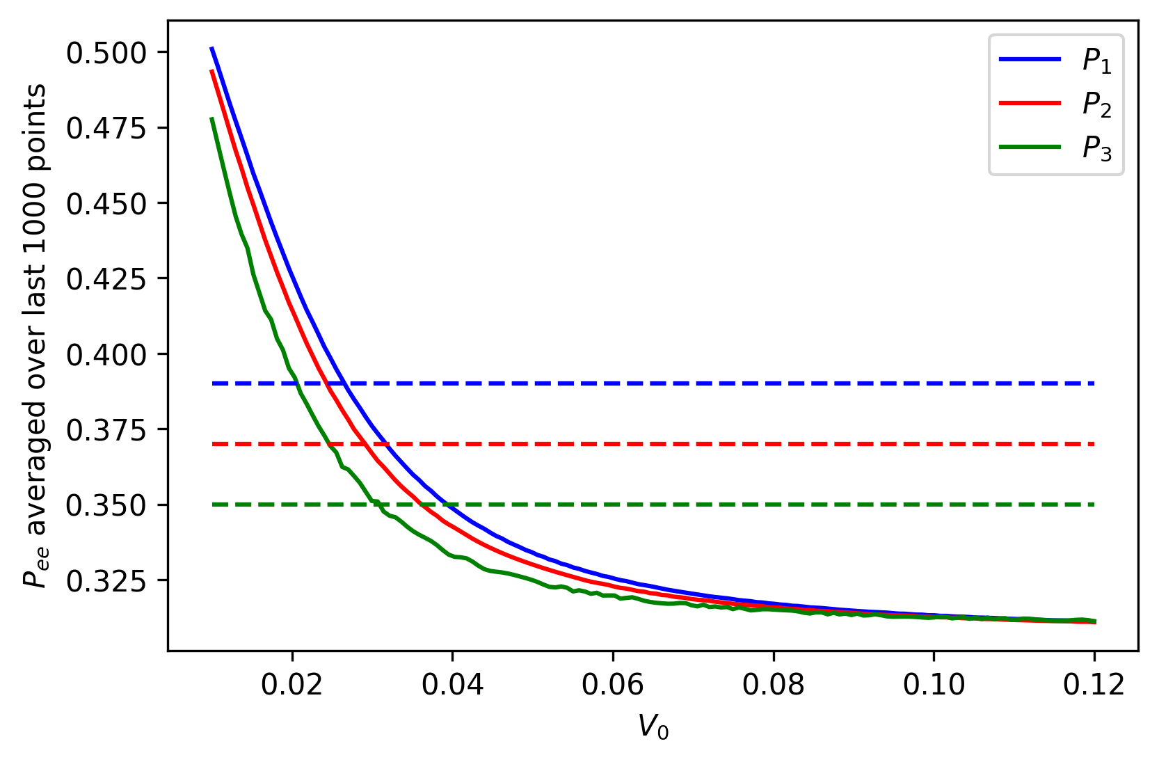
Figure 1: Predicted neutrino survival probabilities $P_{ee}$, as would be measured on Earth based on Eq. (3), versus $V_{0}$, the matter potential at the center of the Sun. These predictions were obtained using forward integration. Dashed lines represent the measured survival probabilities for each neutrino energy in the Borexino experiment Agostini et al. (2018). Here we used the logistic model for $V(r)$ [Eq. (5)]; results for the exponential decay model were visually identical. We used this plot to determine our search range for $V_{0}$. Importantly, this range spans the prediction from the standard solar model Bahcall et al. (2005) of $V_{0}\sim 0.03$ km^-1.

B.   Parameter estimation of $V_{0}$

Once we ascertained that the path of least action reliably corresponded to the best state variable evolution match to the (known) forward integration result in that controlled scenario, and importantly that the reliability did not depend on the value of $V_{0}$ itself (see Sec. V), we proceeded with the more ambitious problem of parameter estimation. Specifically, at this stage we challenged the procedure to infer $V_{0}$, given the (now incomplete) model together with the Borexino data. Here, the permitted search range for $V_{0}$ was: 0.001 to 0.120 km^-1, chosen to match the range used for the preliminary forward integration tests (Fig. 1).

We repeated the parameter estimation, this time considering the Borexino experimental error, by adding Gaussian-distributed noise of that average magnitude into the measurements of $P_{ee}$ at Earth.

We used the open-source Interior-point Optimizer (Ipopt) Wächter (2009) to perform the simulations. Ipopt discretizes the state space via a Hermite-Simpson method, with constant step size. We used 121,901 steps and a step size of $\delta r$ of 2.8524 km^-1. We discretized the state space, and calculated the model Jacobian and Hessian, using a Python interface min that generates C code that Ipopt reads. The computing cluster that ran the simulations had 201 GB of RAM and 24 GenuineIntel CPUs (64 bits), each with 12 cores.

For the proof-of-concept test of the accuracy of the $V_{0}$ estimates, we generated a simulation via forward integration, with all neutrinos initialized at $\left[P_{x},P_{y},P_{z}\right]=\left[0,0,1\right]$ at the solar core. Here we used the value of $V_{0}$ obtained through parameter estimation, and a domain identical to the domain used in the optimization. This result we compared directly to the solution from Ipopt. The integration was performed by Python’s odeINT package, which uses a FORTRAN library and an adaptive step size. Our complete procedure can be found in the publicly available repository of Ref. AA-Ahmetaj .

For all experiments, ten independent paths were initialized randomly. That is, each initialization consisted of as many random choices as there are dimensions to the action surface: $D\times(N+1)+p$, where $D$, $N+1$, and $p$ are the number of state variables, discretized model locations, and parameters, respectively. The permitted search range for state variables ($P_{x}$, $P_{y}$, and $P_{z}$) spanned their full dynamical range: $\left[-1.0,1.0\right]$

V.   RESULTS and DISCUSSION

Key results are threefold:

• For the proof-of-concept experiments wherein $V_{0}$ was taken to be known: the Borexino data were most consistent with a model $V_{0}$ value in the range of 0.025-0.030 km^-1 (in keeping with the prediction from the standard solar model). In addition, the state variable predictions that most closely matched the known result from forward integration were indeed the solutions corresponding to the paths of least action. Thus we had confidence in using the path-of-least-action as a litmus test in the parameter-estimation stage – a stage at which there would exist no independent "known truth" from forward integration.

• For the parameter estimations of $V_{0}$ based on the data: the path-of-least-action litmus test identified a (slightly broader) range for $V_{0}$ that centered around the (smaller) range identified above (of 0.025-0.030 km^-1), as most consistent with the Borexino measurements.

• All results were invariant across the exponential and logistic models for $V(r)$. That is: it was not the shape of the matter profile that dictated the survival probability, but rather only the difference between initial ($V_{0}$) and final ($V_{f}$) values – as expected for adiabatic flavor evolution.

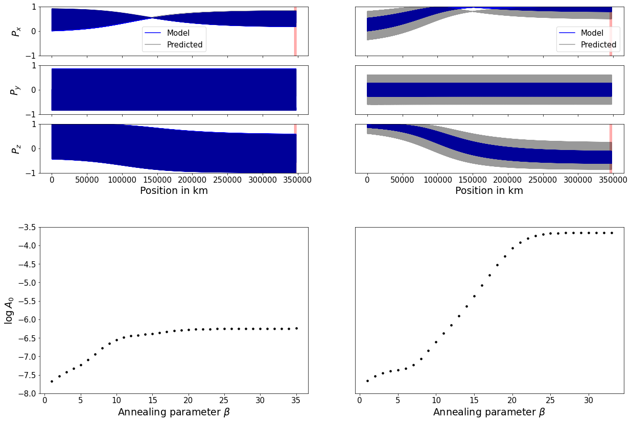
Figure 2: Top: Evolution of state variables, using different fixed values of $V_{0}$ in each case: prediction (gray) versus expectation from forward integration (blue), for one neutrino energy, using the logistic model for $V(r)$. Left: $V_{0}=0.025$ $km^{-1}$; right: $V_{0}=0.095$ $km^{-1}$. The left match is significantly better: black versus blue are indiscernible by-eye. Bottom: Corresponding plots of log(action) versus annealing parameter $\beta$, for each result, respectively. The action asymptotes to $\sim 10^{-6}$ (left) and $\sim 10^{-4}$ (right). Note that the better prediction (left) corresponds to the path of lower action. The exponential model for $V(r)$ yielded similar results; not shown. Thus the action can be taken as a metric for the case of parameter estimation, wherein we will have no independent check on prediction quality from forward integration (since $V_{0}$ will not be considered "known"). In addition, the transparent red band in the panels for $P_{x}$ and $P_{z}$ denote the (sparse) region where measurements of $P_{ee}$ at Earth were provided, as per Eq. (3)

.

A.   Proof of concept: state prediction at fixed $V_{0}$

As described in Sec. IV, our initial step – prior to parameter estimation – was to identify a metric that could be used to identify the optimal solutions for the case wherein the true evolution of state variables is not known. To this end, we ran the optimization for the eight distinct (known) values of $V_{0}$, and compared the resulting predictions for state variables against the (known) results from forward integration.

The top panel of Fig. 2 shows the predicted evolution of state variables (black) compared to the result obtained from integration (blue), for one neutrino energy. Left and right panels are examples of an excellent versus a poorer match, respectively. In both, the overall flavor evolution is qualitatively predicted well, but the prediction on the right fails to capture the amplitude of oscillations. The difference between the procedures on the left versus right was as follows: on the left, the specific model value chosen for $V_{0}$ was 0.025 km^-1; on the right, the choice was instead 0.095 km^-1. (This result was obtained using the logistic form for $V_{0}$; results are similar for the exponential form; not shown.) In other words, these results indicate that a value for $V_{0}$ of 0.025 km^-1 is more compatible with the Borexino measurements, compared to the value of 0.095 km^-1.

Now, the bottom panel of Fig. 2 shows the corresponding plot of the action versus annealing parameter $\beta$, for each result, respectively. The action for the better (left) solution asymptotes to a significantly lower value compared to that at right; namely: $A_{0}\sim 10^{-6}$ compared to $10^{-4}$. Indeed, this was our finding in a much more extensive study of the utility of this "path of least action" for identifying best solutions Armstrong et al. (2020). In addition, note the vertical red band on the plot for $P_{x}$ and $P_{z}$, denoting the region in which measurements were provided to the procedure – as a reminder of their sparsity.

We repeated the comparison shown in Fig. 2 across all chosen values for $V_{0}$. Resulting composite action plots are shown in Fig. 3, for the logistic (top panel) and exponential (bottom) versions. Note that the greater the deviation of the chosen value of $V_{0}$ from the expected range of [0.025, 0.030] km^-1, the higher the action value. And critically: the higher the action value, the poorer the optimization of state variable evolution with the data (not shown). Thus, within the scope of this paper, the action can be taken as a reliable proxy for the correct solution, for the case wherein we "fly blind" without an independent check from forward integration.

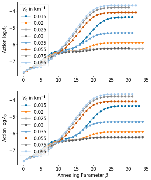
Figure 3: Log of action as a function of annealing parameter $\beta$ for each fixed value of $V_{0}$ chosen in the proof-of-concept stage of optimization, for the logistic [Eq. (5)] model for $V(r)$ (top), and the exponential [Eq. (4)] model (bottom). For both models, values of 0.025 and 0.03 km^-1 resulted in the lowest action, with either lower or higher values of $V_{0}$ corresponding to a higher action plateau.

B.   Parameter estimation of $V_{0}$

With our action-as-litmus-test in hand, we proceeded with parameter estimation of $V_{0}$, given the Borexino data. As per the description in Sec. IV, we performed ten independent trials for each model version of $V(r)$, once without noise, and once with Gaussian noise on the order of the published Borexino errors Agostini et al. (2018) added to the measurements.

Results for the logistic model are shown in Fig. 4 (noiseless) and Fig. 5 (noisy). The top panel of each plot shows the log of the action as a function of $\beta$, for all ten trials. All trials found stable estimates. With the noiseless data, the estimates of $V_{0}$ spanned the range $[0.0105,0.0488]\text{ km}^{-1}$, where the lowest value of the action $A_{0}$ corresponded to an estimate for $V_{0}$ of 0.0247 $\text{ km}^{-1}$. With additive noise, the range for $V_{0}$ was $[0.001,0.0432]\text{ km}^{-1}$, and the value corresponding to lowest action was $V_{0}=0.0243\text{ km}^{-1}$.

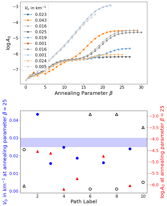
Figure 4: Top: Log of action as a function of annealing parameter $\beta$ for the logistic model, across ten independent trials, without noise in measurements. The values of $V_{0}$ in the plot legend correspond to a value of 25 for annealing parameter $\beta$: an iteration at which solutions had stabilized. Bottom: Estimate of $V_{0}$ [left (blue) $y$-axis, circles] and $\log A_{0}$ at $\beta=25$ [right (red) $y$-axis, triangles], across the ten trials. The light blue band indicates the expected range of $V_{0}$, based on Fig. 1 and on the proof-of-concept optimization runs. (Those trials that did not plateau are denoted by hollow shapes, both for the $V_{0}$ estimates and for the corresponding value of the action.)

Figure 5: Same as Fig. 4 for the logistic model, but showing the results for the optimization trials with Gaussian noise added to the measurements, on the order of the uncertainties in the Borexino data Agostini et al. (2018).

The bottom panels of Figures 4 and 5 offer an alternative display of the information contained in the top panel. Here, the estimate of $V_{0}$ is shown on the left (blue) $y$-axis, and the corresponding asymptotic value of the action is on the right (red) $y$-axis. The horizontal light blue band indicates the expected range for $V_{0}$, based on the analysis depicted in Fig. 1 or 3. Note that the greater the distance of the estimate of $V_{0}$ from that band (blue circle), the higher the action value (red triangle). (Paths whose action value did not reach a stable plateau are denoted with hollow shapes.)

Results for the exponential model were similar: Figures 6 and Fig. 7 show the noiseless and noisy cases, respectively. The without-noise range of estimates for $V_{0}$ was $\left[0.0198,0.0779\right]\,\text{km}^{-1}$, and with noise the range shifted slightly to $\left[0.0173,0.0781\right]\,\text{km}^{-1}$. Again, for both noiseless and noisy cases, the path of least action corresponded to a value for $V_{0}$ within the expected range of $0.025\text{--}0.030$ km^-1.

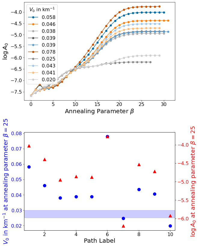
Figure 6: Same as Fig. 4, but with the exponential-decay model for $V(r)$ [Eq. (4)] instead of the logistic model [Eq. (5)], for noiseless measurements.

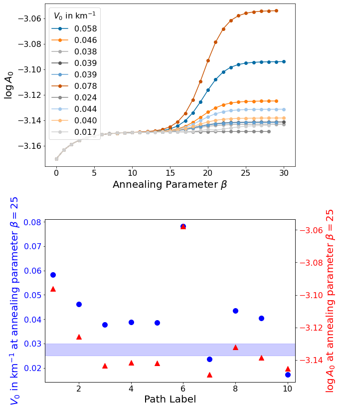
Figure 7: Same as Fig. 6 for the exponential-decay model for $V(r)$ [Eq. (4)], with Gaussian noise added to the measurements, on the order of the Borexino uncertainties Agostini et al. (2018)

In summary, neutrino flavor measurements at terrestrial detectors (e.g., Borexino) can be used to independently constrain the electron density at the solar center (complementary to the existing constraints from stellar oscillations, for instance). This is demonstrated here through a novel application of the SDA method. The outcome is insensitive to the overall shape of the electron density profile, as long as it evolves sufficiently smoothly through the mass level crossing between the instantaneous in-medium neutrino mass eigenstates – ensuring adiabatic flavor evolution across the resonance.

VI.   CONCLUDING REMARKS

The study of stellar oscillations is a growing field. It began as helioseismology, the study of solar oscillations Bahcall and Ulrich (1988). Indeed, there exists a strong connection between helioseismology and neutrino production in the Sun Christensen-Dalsgaard (2002). This connection could be exploited both to learn about nuclear reactions powering the Sun and to learn about the Sun itself Christensen-Dalsgaard (2019); Bellinger and Christensen-Dalsgaard (2022). In particular, observations of pressure waves at the solar surface have grown increasingly precise for deducing the sound speed profile throughout the Sun. Sound speed at any given location in the Sun depends on both matter density and temperature at that location. Hence an accurate determination of the density profile throughout the Sun would require inferring the Sun’s temperature profile.

It is worthwhile to investigate possible improvements that inference might offer for the analysis of solar neutrino data. For example, it might provide an independent check on new methods to remove cosmogenic-induced spallation in Super-Kamiokande, a recent effort to improve the precision of solar neutrino data Locke et al. (2021).

VII.   ACKNOWLEDGEMENTS

C. L., E. A., L. N., S. R., and H. T. acknowledge an Institutional Support for Research and Creativity grant from New York Institute of Technology, and NSF grant 2139004. E. K. J. acknowledges the NSF summer Research Experience for Undergraduates program. The research of A. B. B. was supported in part by the U.S. National Science Foundation Grants No. PHY-2020275 and PHY-2108339. A. V. P. acknowledges support from the U.S. Department of Energy (DOE) under contract number DE-AC02-76SF00515 at SLAC National Accelerator Laboratory and DOE grant DE-FG02-87ER40328 at the University of Minnesota. E. A., A. B. B., and A. V. P. thank the Mainz Institute for Theoretical Physics (MITP) of the Cluster of Excellence PRISMA+ (Project ID 39083149) for its hospitality and support. All co-authors extend gratitude to the good people of Kansas and Doylestown, Ohio.

References

- Balantekin et al. (1988) A. B. Balantekin, S. H. Fricke, and P. J. Hatchell, Phys. Rev. D 38, 935 (1988).
- Fuller et al. (1992) G. M. Fuller, R. Mayle, B. S. Meyer, and J. R. Wilson, Astrophys. J. 389, 517 (1992).
- Qian et al. (1993) Y.-Z. Qian, G. M. Fuller, G. J. Mathews, R. W. Mayle, J. R. Wilson, and S. E. Woosley, Phys. Rev. Lett. 71, 1965 (1993).
- Fuller (1993) G. M. Fuller, Phys. Rept. 227, 149 (1993).
- Fuller and Meyer (1995) G. M. Fuller and B. S. Meyer, Astrophys. J. 453, 792 (1995).
- Balantekin (1999) A. B. Balantekin, Phys. Rept. 315, 123 (1999), arXiv:hep-ph/9808281 .
- Duan et al. (2011) H. Duan, A. Friedland, G. McLaughlin, and R. Surman, J. Phys. G 38, 035201 (2011), arXiv:1012.0532 [astro-ph.SR] .
- Wu et al. (2015) M.-R. Wu, Y.-Z. Qian, G. Martinez-Pinedo, T. Fischer, and L. Huther, Phys. Rev. D 91, 065016 (2015), arXiv:1412.8587 [astro-ph.HE] .
- Wu et al. (2016) M.-R. Wu, G. Martinez-Pinedo, and Y.-Z. Qian, EPJ Web Conf. 109, 06005 (2016), arXiv:1512.03630 [astro-ph.HE] .
- Sasaki et al. (2017) H. Sasaki, T. Kajino, T. Takiwaki, T. Hayakawa, A. B. Balantekin, and Y. Pehlivan, Phys. Rev. D 96, 043013 (2017), arXiv:1707.09111 [astro-ph.HE] .
- Balantekin (2018a) A. B. Balantekin, AIP Conf. Proc. 1947, 020012 (2018a), arXiv:1710.04108 [nucl-th] .
- Balantekin (2018b) A. B. Balantekin, J. Phys. G 45, 113001 (2018b), arXiv:1809.02539 [hep-ph] .
- Xiong et al. (2019) Z. Xiong, M.-R. Wu, and Y.-Z. Qian, (2019), 10.3847/1538-4357/ab2870, arXiv:1904.09371 [astro-ph.HE] .
- Xiong et al. (2020) Z. Xiong, A. Sieverding, M. Sen, and Y.-Z. Qian, Astrophys. J. 900, 144 (2020), arXiv:2006.11414 [astro-ph.HE] .
- Duan et al. (2006) H. Duan, G. M. Fuller, J. Carlson, and Y.-Z. Qian, Physical Review D 74, 105014 (2006).
- Duan et al. (2008) H. Duan, G. M. Fuller, and J. Carlson, Computational Science & Discovery 1, 015007 (2008).
- Richers et al. (2019) S. A. Richers, G. C. McLaughlin, J. P. Kneller, and A. Vlasenko, Physical Review D 99, 123014 (2019).
- Richers et al. (2021a) S. Richers, D. E. Willcox, N. M. Ford, and A. Myers, Phys. Rev. D 103, 083013 (2021a), arXiv:2101.02745 [astro-ph.HE] .
- Richers et al. (2021b) S. Richers, D. Willcox, and N. Ford, Phys. Rev. D 104, 103023 (2021b), arXiv:2109.08631 [astro-ph.HE] .
- Kato et al. (2021) C. Kato, H. Nagakura, and T. Morinaga, Astrophys. J. Supp. 257, 55 (2021), arXiv:2108.06356 [astro-ph.HE] .
- Nagakura (2022) H. Nagakura, Phys. Rev. D 106, 063011 (2022), arXiv:2206.04098 [astro-ph.HE] .
- George et al. (2022) M. George, C.-Y. Lin, M.-R. Wu, T. G. Liu, and Z. Xiong, (2022), arXiv:2203.12866 [hep-ph] .
- Tamborra and Shalgar (2021) I. Tamborra and S. Shalgar, Annual Review of Nuclear and Particle Science 71, 165 (2021).
- Richers and Sen (2022) S. Richers and M. Sen, (2022), arXiv:2207.03561 [astro-ph.HE] .
- Patwardhan et al. (2023) A. V. Patwardhan, M. J. Cervia, E. Rrapaj, P. Siwach, and A. B. Balantekin, “Many-Body Collective Neutrino Oscillations: Recent Developments,” in Handbook of Nuclear Physics, edited by I. Tanihata, H. Toki, and T. Kajino (2023) pp. 1–16, arXiv:2301.00342 [hep-ph] .
- Balantekin et al. (2023) A. B. Balantekin, M. J. Cervia, A. V. Patwardhan, E. Rrapaj, and P. Siwach, Eur. Phys. J. A 59, 186 (2023), arXiv:2305.01150 [nucl-th] .
- Armstrong et al. (2022) E. Armstrong, A. V. Patwardhan, A. A. Ahmetaj, M. M. Sanchez, S. Miskiewicz, M. Ibrahim, and I. Singh, Physical Review D 105, 103003 (2022).
- Armstrong (2022) E. Armstrong, Physical Review D 105, 083012 (2022).
- Armstrong et al. (2017) E. Armstrong, A. V. Patwardhan, L. Johns, C. T. Kishimoto, H. D. I. Abarbanel, and G. M. Fuller, Physical Review D 96, 083008 (2017).
- Armstrong et al. (2020) E. Armstrong, A. V. Patwardhan, E. Rrapaj, S. F. Ardizi, and G. M. Fuller, Physical Review D 102, 043013 (2020).
- Rrapaj et al. (2021) E. Rrapaj, A. V. Patwardhan, E. Armstrong, and G. M. Fuller, Physical Review D 103, 043006 (2021).
- Kimura (2002) R. Kimura, Journal of Wind Engineering and Industrial Aerodynamics 90, 1403 (2002).
- Kalnay (2003) E. Kalnay, Atmospheric modeling, data assimilation and predictability (Cambridge university press, 2003).
- Evensen (2009) G. Evensen, Data assimilation: the ensemble Kalman filter (Springer Science & Business Media, 2009).
- Betts (2010) J. T. Betts, Practical methods for optimal control and estimation using nonlinear programming, Vol. 19 (Siam, 2010).
- Whartenby et al. (2013) W. G. Whartenby, J. C. Quinn, and H. D. I. Abarbanel, Monthly Weather Review 141, 2502 (2013).
- An et al. (2017) Z. An, D. Rey, J. Ye, and H. D. I. Abarbanel, Nonlinear Processes in Geophysics (Online) 24 (2017).
- Schiff (2009) S. J. Schiff, in 2009 Annual International Conference of the IEEE Engineering in Medicine and Biology Society (IEEE, 2009) pp. 3318–3321.
- Toth et al. (2011) B. A. Toth, M. Kostuk, C. D. Meliza, D. Margoliash, and H. D. I. Abarbanel, Biological cybernetics 105, 217 (2011).
- Kostuk et al. (2012) M. Kostuk, B. A. Toth, C. D. Meliza, D. Margoliash, and H. D. I. Abarbanel, Biological cybernetics 106, 155 (2012).
- Hamilton et al. (2013) F. Hamilton, T. Berry, N. Peixoto, and T. Sauer, Physical Review E 88, 052715 (2013).
- Meliza et al. (2014) C. D. Meliza, M. Kostuk, H. Huang, A. Nogaret, D. Margoliash, and H. D. I. Abarbanel, Biological cybernetics 108, 495 (2014).
- Nogaret et al. (2016) A. Nogaret, C. D. Meliza, D. Margoliash, and H. D. I. Abarbanel, Scientific reports 6, 1 (2016).
- Armstrong (2020) E. Armstrong, Physical Review E 101, 012415 (2020).
- Kitiashvili and Kosovichev (2008) I. Kitiashvili and A. G. Kosovichev, The Astrophysical Journal 688, L49 (2008).
- Kitiashvili (2020) I. N. Kitiashvili, in Solar and Stellar Magnetic Fields: Origins and Manifestations, Vol. 354, edited by A. Kosovichev, S. Strassmeier, and M. Jardine (2020) pp. 147–156, arXiv:2003.04563 [astro-ph.SR] .
- Sen et al. (2022) S. Sen, S. Agarwal, P. Chakraborty, and K. P. Singh, Experimental Astronomy 53, 1 (2022).
- Hirata et al. (1987) K. Hirata, T. Kajita, M. Koshiba, M. Nakahata, Y. Oyama, N. Sato, A. Suzuki, M. Takita, Y. Totsuka, T. Kifune, T. Suda, K. Takahashi, T. Tanimori, K. Miyano, M. Yamada, E. W. Beier, L. R. Feldscher, S. B. Kim, A. K. Mann, F. M. Newcomer, R. VanBerg, W. Zhang, and B. G. Cortez, Phys. Rev. Lett. 58, 1490 (1987).
- Bionta et al. (1987) R. M. Bionta, G. Blewitt, C. B. Bratton, D. Casper, A. Ciocio, R. Claus, B. Cortez, M. Crouch, S. T. Dye, S. Errede, G. W. Foster, W. Gajewski, K. S. Ganezer, M. Goldhaber, T. J. Haines, T. W. Jones, D. Kielczewska, W. R. Kropp, J. G. Learned, J. M. LoSecco, J. Matthews, R. Miller, M. S. Mudan, H. S. Park, L. R. Price, F. Reines, J. Schultz, S. Seidel, E. Shumard, D. Sinclair, H. W. Sobel, J. L. Stone, L. R. Sulak, R. Svoboda, G. Thornton, J. C. van der Velde, and C. Wuest, Phys. Rev. Lett. 58, 1494 (1987).
- Alekseev et al. (1987) E. N. Alekseev, L. N. Alekseeva, I. V. Krivosheina, and V. I. Volchenko, in European Southern Observatory Conference and Workshop Proceedings, European Southern Observatory Conference and Workshop Proceedings, Vol. 26 (1987) p. 237.
- Laber-Smith et al. (2023) C. Laber-Smith, A. Ahmetaj, E. Armstrong, A. B. Balantekin, A. V. Patwardhan, M. M. Sanchez, and S. Wong, Physical Review D 107, 023013 (2023).
- Agostini et al. (2018) M. Agostini et al. (BOREXINO), Nature 562, 505 (2018).
- Aharmim et al. (2010) B. Aharmim et al. (SNO), Phys. Rev. C 81, 055504 (2010), arXiv:0910.2984 [nucl-ex] .
- Balantekin et al. (1998) A. B. Balantekin, J. F. Beacom, and J. M. Fetter, Phys. Lett. B 427, 317 (1998), arXiv:hep-ph/9712390 .
- Lopes and Turck-Chièze (2013) I. Lopes and S. Turck-Chièze, Astrophys. J. 765, 14 (2013), arXiv:1302.2791 [astro-ph.SR] .
- Dighe et al. (1999) A. S. Dighe, Q. Y. Liu, and A. Y. Smirnov, (1999), arXiv:hep-ph/9903329 .
- Wolfenstein (1978) L. Wolfenstein, Physical Review D 17, 2369 (1978).
- Bahcall et al. (2005) J. N. Bahcall, A. M. Serenelli, and S. Basu, The Astrophysical Journal 621, L85 (2005).
- Oden and Reddy (2012) J. T. Oden and J. N. Reddy, Variational methods in theoretical mechanics (Springer Science & Business Media, 2012).
- Ye et al. (2015) J. Ye, D. Rey, N. Kadakia, M. Eldridge, U. I. Morone, P. Rozdeba, H. D. I. Abarbanel, and J. C. Quinn, Physical Review E 92, 052901 (2015).
- Wächter (2009) A. Wächter, in Dagstuhl Seminar Proceedings (Schloss Dagstuhl-Leibniz-Zentrum für Informatik, 2009).
- (62) “minAone interface with Interior-point Optimizer,” https://github.com/yejingxin/minAone, accessed: 2020-05-26.
- (63) AA-Ahmetaj, “Slurm_minaone,” https://github.com/AA-Ahmetaj/SLURM_minAone.
- Bahcall and Ulrich (1988) J. N. Bahcall and R. K. Ulrich, Rev. Mod. Phys. 60, 297 (1988).
- Christensen-Dalsgaard (2002) J. Christensen-Dalsgaard, Rev. Mod. Phys. 74, 1073 (2002).
- Christensen-Dalsgaard (2019) J. Christensen-Dalsgaard, in 5th International Solar Neutrino Conference (2019) pp. 81–102, arXiv:1809.03000 [astro-ph.SR] .
- Bellinger and Christensen-Dalsgaard (2022) E. P. Bellinger and J. Christensen-Dalsgaard, Mon. Not. Roy. Astron. Soc. 517, 5281 (2022), arXiv:2206.13570 [astro-ph.SR] .
- Locke et al. (2021) S. Locke et al. (Super-Kamiokande), (2021), arXiv:2112.00092 [hep-ex] .