Abstract

A complete canonical formulation of general covariance makes it possible to construct new modified theories of gravity that are not of higher-curvature form, as shown here in a spherically symmetric setting. The usual uniqueness theorems are evaded by using a crucial and novel ingredient, allowing for fundamental fields of gravity distinct from an emergent space-time metric that provides a geometrical structure to all solutions. As specific examples, there are new expansion-shear couplings in cosmological models, a form of modified Newtonian dynamics (MOND) can appear in a space-time covariant theory without introducing extra fields, and related effects help to make effective models of canonical quantum gravity fully consistent with general covariance.

1 Introduction

General relativity and possible modifications or alternatives, such as quantum gravity corrections, can, to a large extent, be derived from the symmetries of space-time. In the usual formulation based on space-time tensors and Riemannian geometry, the gravitational action must be invariant under coordinate changes and, since it depends on the space-time metric (or alternative geometrical objects such as tetrads or connections), is therefore given by a curvature or torsion invariant. In general relativity, the relevant invariant is proportional to the space-time Ricci scalar plus, perhaps, a cosmological constant. Einstein’s field equation then follows from the variational principle. If higher-order derivatives are included in an effective action that may describe certain quantum effects, higher-curvature actions are obtained in which the Ricci scalar $R$ may be replaced by a non-linear function $f(R)$, and invariants constructed from multiple factors of the full Riemann or torsion tensors are also possible.

For certain aspects of quantum gravity, a canonical formulation is useful because the underlying phase-space structure allows one to look for quantum representations on a Hibert space. Canonical formulations distinguish between configuration degrees of freedom and their velocities, which are turned into momenta as independent phase-space variables. At this basic step, therefore, symmetries such as space-time covariance may not be explicitly realized, but once all dynamical equations have been solved, the solutions are equivalent to those of general relativity and are therefore covariant. The dynamical equations contain, as usual, equations of motion of second order in time derivatives of the metric (or of first order of the configuration variables and momenta), but also constraints that are of at most first order in time derivatives (or contain only spatial derivatives of the canonical fields). Both types of equations follow from specific components of the Einstein tensor, and they can be independently derived in the canonical formulation.

Early, classic work [1, 2, 3, 4] has shown that the constraints are the relevant part of these equations when it comes to symmetries: When the constraints are solved, a condition referred to in this context as going “on-shell,” general covariance can be recovered in the canonical theory from flow equations generated by the constraints. The constraints generate evolution equations as well as gauge transformations by their Hamiltonian vector fields, which on shell are equivalent to space-time coordinate changes. However, the tensorial and canonical formulations are not equivalent off-shell, which may be relevant in particular for an understanding of possible quantum effects that could modify the classical constraint functions in different ways.

Here, we analyze this question in the simpler context of modified gravity and in a reduction to spherically symmetric models. As we will demonstrate, novel covariant theories of modified gravity are then possible, with interesting new phenomena. For instance, there are new types of dynamical signature change [5], and previously constructed models of non-singular black holes [6, 7] can be rederived as special cases. These results help to clarify possible modified-gravity effects implied by canonical quantum gravity. The resulting theories may be of interest also for purely classical questions, for instance by providing new covariant equations for phenomenological applications that cannot be obtained from traditional versions of modified gravity.

Physically, new theories of modified gravity are possible in a canonical formulation because setting up a canonical theory of gravity requires weaker assumptions than what is used to specify an action. Any tensorial formulation of gravity by an action principle has to start with a fundamental space-time tensor, usually the metric, on which the Lagrangian depends and which defines the integration measure for the action. A canonical formulation of gravity, by contrast, can be given with fewer assumptions because it only requires suitable spatial tensors with a phase-space structure, and only spatial integrations in the Hamiltonian and diffeomorphism constraints. Unlike in a tensorial formulation, in which general covariance is built into the formalism by making use of the tensor transformation law in space-time, general covariance in a canonical formulation is a derived concept that must be demonstrated by an analysis of Poisson brackets and gauge flows of the constraints. While this property makes it harder to construct covariant theories of gravity in purely canonical form, it also provides an opening to new theories of modified gravity because a canonical formulation starts with weaker requirements on the fundamental fields.

In particular, we will see that it is possible to relax the usual identity between the fundamental canonical configuration field and the induced spatial metric of the corresponding space-time geometry. This identity is realized in all higher-curvature formulations of modified gravity, but it is not necessary in a broader setting of modified canonical gravity. In these new theories, the space-time metric, or even its spatial part, is not fundamental but rather emergent. Even if it does not agree with a canonical configuration variable, the emergent spatial metric $q_{ab}$ is uniquely determined by the structure function of the Poisson bracket of two Hamiltonian constraints.

Moreover, the canonical realization of general covariance works by reconstructing space-time transformations from deformations of spatial hypersurfaces in normal and tangential directions. In a canonical formulation of a theory defined by an action principle directly for the space-time metric or tetrad, such as general relativity or some higher-curvature theory, the normal direction, just as the induced spatial metric on a hypersurface, is uniquely determined by the fundamental space-time metric. If one tries to construct consistent gravity theories purely in a canonical setting, the normal direction is defined more abstractly through the rules by which general covariance is implemented canonically, related to the algebraic form of different Poisson brackets of the constraints that define the theory. In the absence of a fundamental space-time metric, it turns out, this definition of the normal direction $n^{a}$ is no longer unique and may allow inequivalent realizations of a geometrical space-time structure. Each realization results in a consistent and covariant gravitational theory with an emergent space-time metric subject to the full set of coordinate transformations, defined by the usual combination $g_{ab}=q_{ab}-n_{a}n_{b}$ where both objects on the right are now emergent, $q_{ab}$ from the structure function and $n_{a}$ from what has been specified as the Hamiltonian constraint. But different realizations imply inequivalent emergent space-time metrics not mutually related by coordinate changes. In practice, different choices of normal directions can be parameterized by replacing the original constraints of canonical general relativity with suitable linear combinations subject to phase-space dependent coefficients.

Such linear combinations therefore present a new, previously unrecognized approach to modified gravity. This outcome is surprising because one usually thinks of the constraints as generators of some algebraic structure, which should be invariant under linear combinations of the generators. However, equipping solutions with a geometrical structure via the emergent spatial metric and normal direction is an additional ingredient that may well be (and, as we will show explicitly, is) sensitive to which linear combinations of algebraic generators are distinguished as the specific Hamiltonian and diffeomorphism constraint whose gauge transformations correspond to normal and tangential directions of spatial hypersurfaces. The well-known structure function in the Poisson bracket of two Hamiltonian constraints then determines the emergent space-time metric which, subject to strong consistency conditions, also depends on which linear combination of the generators is singled out as the Hamiltonian constraint.

Since the foundation of our new theories of emergent modified gravity depends crucially on these canonical structures and properties of hypersurface deformations, we will begin with a detailed review of relevant properties in the next section. The resulting new spherically symmetric theories, along with some solutions, will then be evaluated for new physics effects, considering expansion and shear terms in cosmological models as well as regimes of intermediate-strength gravity. Some of the new terms could be implied by various ingredients of quantum gravity, but a purely classical interpretation is also possible in which novel covariant modifications can be made available for phenomenological studies. The main motivation of emergent modified gravity then consists in the observation that the space-time metric need not be one of the fundamental fields in an action principle while maintaining the symmetry condition of general covariance. From the perspective of effective field theory, any new terms made possible by this more general viewpoint should then be included in physical evaluations, especially in tests of strong-field gravity.

2 Hypersurface deformations

Following [4], the gauge symmetries of the canonical formulation of general relativity can be identified with hypersurface deformations of constant-time spatial slices in space-time, operating in normal and tangential directions. Since a coordinate transformation in general changes the notion of constant-time slices, hypersurface deformations are related to coordinate transformations. In practice, indeed, standard methods to analyze solutions of general relativity may refer to coordinate transformations or to choosing a slicing of space-time into a collection of spatial hypersurfaces without making much of a conceptual distinction. However, while a coordinate choice in particular of time defines a slicing through constant-time hypersurfaces, the deformation of a hypersurface in its normal direction is, in general, not the same as a coordinate change in the time direction. For a given geometrical structure of space-time, it is not difficult to translate these two notions into each other. But the construction of new gravitational theories is more involved because a pre-existing space-time structure cannot be taken for granted.

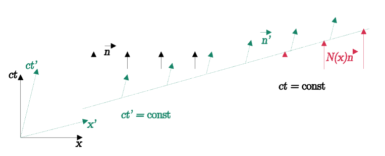
Figure 1: Deformations of constant-time spatial slices in Minkowski space-time are equivalent to Poincaré transformations. Spatial slices of constant $t$ and $t^{\prime}$, related by a Lorentz boost, define different hyperplanes in Minkowski space-time. Their unit normals $\vec{n}$ and $\vec{n}^{\prime}$, respectively, are defined by the indefinite Minkowski scalar product. A boost can be described geometrically by a deformation of the initial slice by a position-dependent deformation of length $N(x)$ in the normal direction, introducing the lapse function $N(x)$. Similarly, spatial translations and rotations are determined by a shift vector field $\vec{w}$ tangential to a spatial hypersurface. Combining a pair of hypersurface deformations in the two possible orderings implies a commutator that is equivalent to the algebraic Lie bracket in the Poincaré algebra. The example shown here represents a geometrical version of the time deformation $T(N)$, which leads to the commutator (3) for linear $N(x)$ and a Euclidean spatial metric in the case of special relativity.

In the simpler case of special relativity, in which the Minkowski space-time metric is constant in Cartesian coordinates and only linear transformations are considered, the symmetries of the Poincaré algebra can be shown to be equivalent to hypersurface deformations, as illustrated in Fig. 1. But the relationship between hypersurface deformations and space-time transformations is more complicated if one goes beyond this setting by allowing for non-Cartesian coordinates or space-time curvature. At first sight, the transition to general relativity looks simple: Hypersurface deformations can easily be generalized to non-planar spatial hypersurfaces in curved space-time and their deformations along normal and tangential directions. As illustrated in Fig. 2, given a background space-time metric in which these deformations take place, one can compute geometrical commutators of pairs of such deformations. Using $S(\vec{w})$ to denote an infinitesimal spatial deformation by a shift vector field $\vec{w}$ tangential to a hypersurface, and $T(N)$ to denote a timelike deformation along the unit normal by a lapse function $N$, the well-known result is given by the equations [1, 2, 3]

$$[S(\vec{w}_{1}),S(\vec{w}_{2})] = S({\cal L}_{\vec{w}_{1}}\vec{w}_{2})$$ (1)

$${}[T(N),S(\vec{w})] = -T({\cal L}_{\vec{w}}N)$$ (2)

$${}[T(N_{1}),T(N_{2})] = S(N_{1}\nabla N_{2}-N_{2}\nabla N_{1})$$ (3)

where ${\cal L}_{\vec{w}}$ is the standard directional or Lie derivative along the vector field $\vec{w}$.

Figure 2: Normal deformations of spatial hypersurfaces in curved space-time. Applying a pair of normal deformations with lapse functions $N_{1}$ and $N_{2}$, respectively, in the two different orderings implies a non-zero spatial deformation tangential to the final hypersurface of the form (3). The normal angle is shown based on local Minkowski geometry, following Fig. 1. In general relativity, the functions $N(x)$ need not be linear, and induced spatial metrics on hypersurfaces may be curved. The displacement vector $\vec{w}$ then depends on the spatial metric through the gradients of $N_{1}$ and $N_{2}$ in (3).

While the last equation, (3), looks quite simple, it complicates the underlying mathematical structure because, unlike the Lie derivatives in the first two equations, the gradient $\nabla N$ of a function $N$ requires a metric. Such a metric is available, given by the spatial metric

$$q_{ab}=g_{ab}+n_{a}n_{b}$$ (4)

induced by the space-time metric $g_{ab}$ on an embedded hypersurface with unit normal $n^{a}$. But its presence in (3) means that the commutator not only depends on the generating functions $N$ and $\vec{w}$ that define hypersurface deformations, but also on the geometry on the hypersurface. In the physics literature, such a bracket is usually referred to as “open” or one with “structure functions.” To close the brackets, we have to be able to apply commutators multiple times, which, since the spatial metric appears in $S$ on the right-hand side of (3), requires that $N$ and $\vec{w}$ should be allowed to depend on the metric, in addition to their dependence on coordinates. With this additional dependence, the set of generators is larger than what the four space-time directions would initially indicate. (Mathematically, the metric dependence can be formulated by using the notion of algebroids, in which (1)-(3) are realized as brackets on sections of a fiber bundle over a suitable space of metrics. However, as shown recently [8] in an application of general mathematical results to the case of hypersurface deformations, the corresponding bracket, placed in the language of BRST/BFV gauge generators, cannot be Lie but is $L_{\infty}$.)

For our new results, the appearance of the spatial metric in the structure function of an algebraic bracket turns out to be a crucial ingredient. If we start from scratch in order to define a canonical theory by finding expressions for $S(\vec{w})$ and $T(N)$ in agreement with (1)–(3), we will have to assume a certain phase space on which these expressions are defined, using Poisson brackets to compute a realization of the required commutators. However, since the spatial metric appears in the structure function of any set of generators that has the form of (1)–(3), we do not have to make assumptions about which phase-space function can play the role of a spatial metric. The geometrical structure of solutions, if it exists given consistency conditions described below, is therefore a derived concept in canonical gravity and need not be presupposed. This conclusion would not be possible if the generators had formed a Lie algebra with structure constants.

In practice, we usually do not try to invent completely new constraints that could have a chance of obeying (1)–(3). We rather start with the known classical constraints of a gravity theory in canonical form, and try to modify them so as to preserve as much of the structure of their Poisson brackets. This condition together with other requirements of general covariance is very restrictive, as shown for instance in several discussions related to models of loop quantum gravity [9, 10, 11] which, as we will describe below, did not even include all the required covariance conditions. In these examples, the main modification consisted in a non-polynomial dependence of the Hamiltonian constraint or the generator $T(N)$ on the classical expression for extrinsic curvature. While partial realizations of such modified covariant models were possible in vacuum spherical symmetry, an extension to models with local degrees of freedom, such as spherical symmetry with scalar matter or polarized Gowdy models, turned out to be difficult.

A different way of modifying canonical gravity has been implicitly suggested by recent work on spherically symmetric models [12, 13, 6, 7], building on the older [14] and [11]. The constructions in [6, 7] used different ingredients not considered in what follows, such as non-bijective canonical transformations, but the crucial step, as we will demonstrate, was an apparently innocuous application of linear combinations of the original constraints with phase-space dependent coefficients. Such coefficients, or equivalently a phase-space dependence of $N$ or $\vec{w}$ in $T(N)$ and $S(\vec{w})$, changes the brackets (1)–(3). For instance, if $N_{1}$ and $N_{2}$ depend on the phase-space degree of freedom $q$ that classically represents the spatial metric, the Poisson bracket $\{T(N_{1}),T(N_{2})\}$ contains terms of the form $T(\partial N/\partial q)$ in contrast to (3). Such terms vanish on-shell, but they are relevant for the off-shell brackets and possible space-time geometries that could be reconstructed from them. If there is a contribution from $T$ to the right-hand side of (3), the bracket does not have the form required for hypersurface deformations, even if it is still closed (and therefore anomaly-free in the sense of gauge transformations). However, it may be possible to remove such terms by further modifications of the generators, in particular replacing the $T(N)$ that one identifies with the Hamiltonian constraint with a linear combination of the original $T(N)$ and $S(\vec{w})$, both with phase-space dependent coefficients. The form (3) may then be recovered, although in general the structure function does not equal the original phase-space degree of freedom $q$ (or its inverse).

Crucially, unlike in an algebraic bracket in which $T(N)$ is just one of the generators, the canonical reconstruction of a space-time geometry depends on which expression $T(N)$ one considers to represent normal deformations. Singling out a specific $T(N)$ with phase-space dependent $N$ as the Hamiltonian constraint, or a specific linear combination of both $T(N)$ and $S(\vec{w})$ with phase-space dependent coefficients, defines the normal direction of hypersurfaces. The choice can therefore have an effect on the resulting reconstructed space-time geometry. Similarly, if the structure function in (3) is modified, the geometry of hypersurface deformations implies that the inverse of the new structure function has to be identified with the spatial metric of a reconstructed space-time line element. Physical evaluations of versions of $T(N)$ with different dependencies of $N$ on the spatial metric are not guaranteed to be equivalent to one another because they imply different space-time metrics from the canonical ingredients, given by the definition of a normal direction through the choice of $T(N)$ and the spatial metric derived from the structure function in (3). Since the space-time line element is derived in this situation and does not agree with the original phase-space degrees of freedom, we refer to it as an emergent line element.

This new and unexpected feature makes it possible to look for novel theories of modified gravity that are not of the form of higher-curvature or other action-based theories. Instead of starting with a space-time tensorial object such as a metric or connection and then looking for invariant action functionals depending on these basic fields, emergent modified gravity starts with a phase space suitable for gravitational fields and derives a compatible object for space-time geometry as well as its dynamics. This object may depend non-trivially on the basic fields, generalizing the usual construction method based on action principles. In what follows, we confirm this expectation by an explicit construction in the setting of spherically symmetric gravity, highlighting consistency conditions that make it possible to construct an emergent line element invariant under the full set of coordinate transformations. Our examples will reveal new effects in cosmological models as well as modified Newtonian gravity in a covariant theory.

3 Covariance and emergent line elements

Spherically symmetric gravity can be described by line elements

$${\rm d}s^{2}=-N(t,x)^{2}{\rm d}t^{2}+\frac{e_{2}(t,x)^{2}}{e_{1}(t,x)}({\rm d}x+w(t,x){\rm d}t)^{2}+e_{1}(t,x){\rm d}\Omega^{2}$$ (5)

where $e_{1}>0$, $e_{2}$, $N$ and $w$ are functions of the time coordinate $t$ and the radial coordinate $x$ but do not depend on the polar angles $\vartheta$ and $\varphi$ that appear in ${\rm d}\Omega^{2}={\rm d}\vartheta^{2}+\sin^{2}\vartheta{\rm d}\varphi^{2}$. The momenta $k_{1}$ and $k_{2}$, canonically conjugate to $e_{1}$ and $e_{2}$, respectively, also depend only on $t$ and $x$. Explicit phase-space expressions classically realizing $T(N)$ and $S(w)$ as functions of $e_{i}$ and $k_{i}$ are given by [15]

$$T[N]=\int{\rm d}x\ N\bigg{(}-\frac{e_{2}k_{2}^{2}}{2\sqrt{e_{1}}}-2k_{2}\sqrt{e_{1}}k_{1}-\frac{\sqrt{e_{1}}e_{1}^{\prime}e_{2}^{\prime}}{2e_{2}^{2}}+\frac{\sqrt{e_{1}}e_{1}^{\prime\prime}}{2e_{2}}+\frac{(e_{1}^{\prime})^{2}}{8\sqrt{e_{1}}e_{2}}-\frac{e_{2}}{2\sqrt{e_{1}}}\bigg{)}$$ (6)

and

$$S[w]=\int{\rm d}x\ w\left(k_{2}^{\prime}e_{2}-k_{1}e_{1}^{\prime}\right)$$ (7)

(using units in which Newton’s constant equals one). Their Poisson brackets obey (3) provided $N$ and $w$ do not depend on $e_{i}$ and $k_{i}$. Equations of motion generated by these constraints identify $k_{1}$ and $k_{2}$ with suitable components of extrinsic curvature, but this relationship is in general modified when new expressions for $T[N]$ and $S[w]$ are used.

Motivated by the discussion of the previous section, we now implement a specific linear transformation of the classical generators $T(N)$ and $S(w)$, represented by (6) and (7), by replacing them with $T(N^{\prime})$ and $S(w^{\prime})$ with $N^{\prime}=\alpha N$ and $w^{\prime}=\beta N+w$, where $\alpha$ and $\beta$ are allowed to depend on $(e_{i},k_{i})$. (Without loss of generality, we will assume that the original $N$ and $w$ are not phase-space dependent.) In terms of the old $N$ and $w$, the new combined generator

$$T(N^{\prime})+S(w^{\prime})=[T(\alpha N)+S(\beta N)]+S(w)$$ (8)

contains an unchanged spatial deformation $S(w)$, but the previous normal deformation $T(N)$ is replaced by $T^{\prime}(N)=T(\alpha N)+S(\beta N)$. If it is possible to reconstruct a generally covariant space-time geometry from the new normal direction and the resulting structure function, it will be different from the classical line element defined by (5) even though it will be a gravitational theory for the same fields $e_{1}$, $e_{2}$ and $N$.

In order to make sure that the transformed generators still define a space-time geometry suitable for a gravitational theory, such that solutions are generally covariant in the usual sense and can be described by invariant line elements familiar from Riemannian geometry, we must show that $T(N^{\prime})$ and $S(w^{\prime})$ still have Poisson brackets of the form (1)–(3). Any extra terms from phase-space derivatives of $\alpha$ and $\beta$ must therefore combine in the correct way for the right-hand sides of (1)–(3) to appear. If this is the case, there may still be deviations in the precise coefficients, in particular in (3) where a different structure function may appear instead of the inverse spatial metric of (5) used in the gradient. Therefore, traditional uniqueness results going back to [1] need not apply, opening up the possibility of new modified theories of gravity. However, a modified gravity theory of classical type, described by a line element, must still be generally covariant. The final task of showing that a modified theory is well-defined then consists in demonstrating that its gauge transformations, generated by $T(N^{\prime})$ and $S(w^{\prime})$, are equivalent to coordinate changes in an emergent line element distinct from (but depending on) the fundamental canonical fields.

These tasks, computing the Poisson brackets and checking gauge transformations, are lengthy exercises, but they are unambiguous because the expressions for $T$ and $S$ are explicitly known. (See [16] for more details.) The result is that the theory may indeed be modified in new ways, but with restrictions that limit the initial freedom of two functions, $\alpha$ and $\beta$. The covariance condition requires

$$\alpha(e_{1},k_{2})=\sqrt{1-s\lambda(e_{1})^{2}k_{2}^{2}}$$ (9)

where $s=\pm 1$ is a sign choice and $\lambda$ a free function of $e_{1}$. (We are dropping a possible multiplier of the square root that would be allowed to depend only on $e_{1}$. The same multiplier would appear in $\beta$ and simply rescale $T(N^{\prime})$.) The second function, $\beta$, is then completely determined and equals

$$\beta(e_{1},k_{2})=\frac{\sqrt{e_{1}}}{2e_{2}^{2}}\frac{\partial e_{1}}{\partial x}\frac{s\lambda(e_{1})^{2}k_{2}}{\sqrt{1-s\lambda(e_{1})^{2}k_{2}^{2}}}\,.$$ (10)

Given these functions, the Poisson-bracket version of (3) produces an expression related to $S(\vec{w})$, but its coefficients do not exactly equal those in (3), where $\nabla N=q^{xx}\partial N/\partial x$ and $q^{xx}=e_{1}/e_{2}^{2}$ from (5) in spherical symmetry. It rather equals a similar expression in which the inverse of

$$q^{\rm em}_{xx}=\left(1+\frac{1}{4e_{2}^{2}}\frac{s\lambda(e_{1})^{2}}{1-s\lambda(e_{1})^{2}k_{2}^{2}}\left(\frac{\partial e_{1}}{\partial x}\right)^{2}\right)^{-1}\frac{e_{2}^{2}}{e_{1}}$$ (11)

replaces $q^{xx}$. We thus derived an emergent metric, (11), distinct from the classical field $q_{xx}$, for which a detailed analysis building on [11] shows that its coordinate transformations are consistent with gauge transformations generated by $T(N^{\prime})$ and $S(w^{\prime})$. (The field $q_{xx}$ can no longer be interpreted as a metric or some other space-time tensor because its gauge transformations do not imply the tensor transformation law. There is a single metric in our modified gravity theories, given by $q^{\rm em}_{xx}$, which are therefore not of bimetric form.) If $\alpha$ and $\beta$ do not obey (9) and (10), there is no emergent metric that obeys this condition, and the theory cannot be covariant or geometrical.

These results already demonstrate that we have arrived at a new class of modified gravity theories. They clearly have general relativity as a limit $\lambda\to 0$, and have solutions with nearly standard behavior in regimes in which $\lambda$ or its multipliers in (9), (10) and (11), such as $k_{2}$, are small. The fact that the emergent metric of a covariant line element for solutions of these theories does not agree with the basic field $q_{xx}=e_{2}^{2}/e_{1}$ in the constraints implies that such theories cannot follow from a space-time action principle of the usual form: The latter would require a space-time metric in order to define the integration measure. But since the correct metric is emergent and not fundamental, the variation of the metric has to be done with respect to the fundamental fields rather than the metric to obtain the equations of motion. Since this procedure cannot provide the expression for the emergent metric which is not known a priori, there is no fundamental action principle. This observation also demonstrates the more general nature of emergent modified gravity compared with conventional modifications: In the latter case, the spatial metric would, by assumption, be given by the fundamental fields, such as $q_{xx}=e_{2}^{2}/e_{1}$ in triad variables. A direct comparison with (11) shows that this assumption is compatible only with the case of $\lambda=0$, ruling out any modifications of the kind studied here. However, this outcome is a consequence only of the assumption that fundamental fields directly determine the spatial metric. It is not implied by general covariance of the resulting gravitational theory.

If the emergent metric were known, we could use it for the integration measure, while the equations of motion are obtained by varying with respect to the fundamental fields. But to the best of our knowledge, the emergent metric cannot be obtained from purely variational arguments. The fundamental fields ($e_{1}$ and $e_{2}$) are distinct from the emergent metric ($q_{xx}^{\rm em}$), just as the physical significance of matter, given by the stress-energy tensor, is distinct from the fundamental fields that define it. Yet, the field equations as well as covariance transformations are completely determined by the constraints and their canonical structure, derivable from Poisson brackets. These properties are in contrast to standard modified gravity theories, such as $f(R)$ or TeVeS, which modify the dynamics but not the structure of space-time because they all assume that the metric is a fundamental field by necessity.

Any new class of modified gravity theories implies a wealth of applications, in comparisons with observations or as models of various effects of quantum gravity. In particular, new effects are not necessarily restricted to large curvature. We will present a few examples in what follows.

4 Applications

We first briefly mention two implications of our modifications that depend on characteristic details of the function (9) and the metric (11), and suggest how emergent modified gravity may differ from standard modifications. These features depend on the sign factor $s$. If $s=1$, the function (11) cannot be negative and may directly be used as an inverse spatial metric. For $s=-1$, however, there may be solutions for which (11) changes sign and becomes negative for certain ranges of $x$. This possibility has been demonstrated explicitly in [5]. The sign then implies signature change, derived dynamically from a covariant theory of gravity. This possibility cannot appear if the structure of space-time is presupposed before an action principle is defined.

If $s=1$, the functional form (9) together with reality conditions implies that the curvature component $k_{2}$ must be bounded. While this outcome may also be obtained for certain solutions of higher-curvature theories, such as [17], here it is generic for all solutions provided $s=1$. We can relate this result to a recent construction [6, 7] of modified spherically symmetric solutions that turns out to be a special case of our new class. If we choose $\lambda(e_{1})=\lambda$ constant in addition to $s=1$, we can apply the canonical transformation

$$k_{2}=\frac{\sin(\lambda k^{\prime}_{2})}{\lambda}\quad,\quad e_{2}=\frac{e_{2}^{\prime}}{\cos(\lambda k_{2}^{\prime})}$$ (12)

and obtain $\alpha=\cos(\lambda k_{2})$. In this form, the example of covariant modified gravity had been used in [6, 7] in order to construct a non-singular black-hole model, but the origin of the modification remained unclear. Initially it seemed that it may be a consequence of the non-invertible canonical transformation (12), but this possibility had already been ruled out in [18] in a discussion of the earlier [19]. Our results clarify that the modification of gravity in the model of [6, 7] is indeed genuine and relies not on a canonical transformation but rather on a linear, phase-space dependent transformations of generators that redefines the normal direction of hypersurface deformations, compared with the classical geometry.

4.1 General modifications

More generally, we may try to modify the classical expression of $T(N)$ before we apply a linear transformation (8). For instance, as suggested in models of loop quantum gravity [20, 9], we could replace the quadratic dependence on curvature components in $T(N)$ by non-classical polynomials or even non-polynomial functions, motivated by quantum-gravity considerations. (In the canonical setting, higher-order expressions of curvature, given by momentum components, do not imply higher time derivatives, unlike space-time tensorial higher-curvature actions.) On its own, such a modification cannot easily be reconciled with general covariance [11], but the combination with a suitable linear transformation (8) turns out to help. Again, this is possible only thanks to the underlying geometrical behavior of normal directions and emergent metrics, because from a purely algebraic perspective the linear transformation would not be able to adjust gauge transformations so as to agree with coordinate changes of an emergent line element. The main outcome, see again [16] for details, is that the emergent metric component (11) can be generalized to

$$q^{\rm em}_{xx}(e_{1},e_{2},k_{2})=\left(f(e_{1})+\frac{\bar{\lambda}^{2}}{4e_{2}^{2}}\left(\frac{\partial e_{1}}{\partial x}\right)^{2}\right)^{-1}\frac{1}{\cos^{2}\left(\bar{\lambda}k_{2}\right)}\frac{e_{2}^{2}}{e_{1}}$$ (13)

with a new free function $f(e_{1})$, while $\bar{\lambda}$ is now constant. (This constant is indirectly related to the previous $\lambda(e_{1})$ by a canonical transformation of the phase-space functions [16]. If the expression on the right is not positive definite, the spatial metric is given by its absolute value and the sign determines the signature of space-time.) The emergent spatial metric (13) is realized by a Hamiltonian constraint of the form

$$T[N] = -\frac{1}{2}\int{\rm d}xN\sqrt{e_{1}}\Bigg{(}e_{2}f_{0}+e_{2}\left(2\frac{{\rm d}f}{{\rm d}e_{1}}+\frac{f\alpha_{2}}{e_{1}}\right)\frac{\sin^{2}\left(\bar{\lambda}k_{2}\right)}{\bar{\lambda}^{2}}+4fk_{1}\frac{\sin(2\bar{\lambda}k_{2})}{2\bar{\lambda}}$$

$$-\frac{(e_{1}^{\prime})^{2}}{e_{2}}\left(\frac{\alpha_{2}}{4e_{1}}\cos^{2}\left(\bar{\lambda}k_{2}\right)-\frac{k_{1}}{2e_{2}}\bar{\lambda}\sin\left(2\bar{\lambda}k_{2}\right)\right)+\left(\frac{e_{1}^{\prime}e_{2}^{\prime}}{e_{2}^{2}}-\frac{e_{1}^{\prime\prime}}{e_{2}}\right)\cos^{2}\left(\bar{\lambda}k_{2}\right)\Bigg{)}\,.$$

Only terms up to second order in spatial derivatives have been considered in the derivation. For higher derivative orders, there may be additional modified theories for instance of Horndeski type [21, 22, 23]. The modifications studied here imply second-order field equations, by construction, but they are not included in Horndeski-type theories because their emergent space-time metric differs from the fundamental fields. Indeed, the crucial Horndeski term of the form $(\nabla^{\mu}\phi)(\nabla^{\nu}\phi)\nabla_{\mu}\nabla_{\nu}\phi$ with a scalar field $\phi$ does not appear in $T[N]$. In a dilaton interpretation, the role of $\phi$ could be played by $e_{1}$ here, but the terms included do not have a sufficient number of derivatives for a dilaton-Horndeski theory [24].

The free functions $f_{0}$ and $\alpha_{2}$ both depend on $e_{1}$ and play different roles. The function $f_{0}$ generalizes the classical dilaton potential and can also be used to include a cosmological constant. The function $\alpha_{2}$ is restricted by the condition that it approaches the value one in the correct low-curvature limit and has no classical analog. It is similar to $\alpha$-parameters derived for modified canonical theories in [25], which can be obtained here in the limit $\bar{\lambda}=0$. Since $\alpha_{2}\not=1$ changes the relative weights between the two $k$-terms in $T[N]$, one depending only on $k_{2}$ and one linear in $k_{1}$, this function may also be interpreted as a modification of Hořava–Lifshitz type [26], but one that preserves general covariance through the emergent line element. Like the previous (11), the right-hand side of (13) is not guaranteed to be positive for all admissible choices of $f$. We restrict attention here to the case in which the right-hand side of (13) is positive, as required for a spatial metric. The more general case and the related phenomenon of signature change are discussed in [16].

Given the free functions, the resulting modified theories can be analyzed in different ways, depending on physical applications. In order to facilitate intuitive interpretations, we first continue with the general theory but rewrite the expressions of the emergent metric and the Hamiltonian constraint in terms of time derivatives of $e_{1}$ and $e_{2}$ replacing the momenta $k_{1}$ and $k_{2}$ upon using equations of motion. For simplicity, we assume a vanishing shift function. The relevant equations of motion are

$$\frac{\dot{e}_{1}}{N}=2\sqrt{e_{1}}\left(f+\frac{\bar{\lambda}^{2}(e_{1}^{\prime})^{2}}{4e_{2}^{2}}\right)\frac{\sin(2\bar{\lambda}k_{2})}{2\bar{\lambda}}$$ (15)

and

$$\frac{\dot{e}_{2}}{N} = \sqrt{e_{1}}\Bigg{(}2e_{2}\frac{{\rm d}f}{{\rm d}e_{1}}-\bar{\lambda}^{2}\left(\frac{e_{1}^{\prime}e_{2}^{\prime}}{e_{2}^{2}}-\frac{e_{1}^{\prime\prime}}{e_{2}}\right)\Bigg{)}\frac{\sin(2\bar{\lambda}k_{2})}{2\bar{\lambda}}$$ (16)

$$+2k_{1}\sqrt{e_{1}}\left(f+\bar{\lambda}^{2}\frac{(e_{1}^{\prime})^{2}}{4e_{2}^{2}}\right)\cos(2\bar{\lambda}k_{2})+\frac{e_{2}}{2}\frac{\alpha_{2}}{e_{1}}\frac{\dot{e}_{1}}{N}\,.$$

The first equation, upon using

$$\cos^{2}(\bar{\lambda}k_{2})=\frac{1}{2}\left(1+\sqrt{1-\sin^{2}(2\bar{\lambda}k_{2})}\right)\,,$$ (17)

can directly be used to write the emergent radial metric as

$$q^{\rm em}_{xx}=\left(f+\bar{\lambda}^{2}\frac{(e_{1}^{\prime})^{2}}{4e_{2}^{2}}+\sqrt{\left(f+\frac{\bar{\lambda}^{2}(e_{1}^{\prime})^{2}}{4e_{2}^{2}}\right)^{2}-\bar{\lambda}^{2}\frac{\dot{e}_{1}^{2}/N^{2}}{e_{1}}}\right)^{-1}\frac{2e_{2}^{2}}{e_{1}}\,.$$ (18)

In this form, the metric depends not only on the gravitational configuration variables, $e_{1}$ and $e_{2}$, but also on their first-order space and time derivatives.

The coefficients in $T[N]$ are then given in terms of

$$\frac{\sin(2\bar{\lambda}k_{2})}{2\bar{\lambda}}=\frac{\dot{e}_{1}/N}{2\sqrt{e_{1}}(f+\frac{1}{4}\bar{\lambda}^{2}(e_{1}^{\prime})^{2}e_{2}^{-2})}$$ (19)

and

$$\cos(2\bar{\lambda}k_{2})=\frac{\sqrt{e_{1}\left(f+\frac{1}{4}\bar{\lambda}^{2}(e_{1}^{\prime})^{2}e_{2}^{-2}\right)^{2}-\bar{\lambda}^{2}\dot{e}_{1}^{2}/N^{2}}}{\sqrt{e_{1}}(f+\frac{1}{4}\bar{\lambda}^{2}(e_{1}^{\prime})^{2}e_{2}^{-2})}$$ (20)

as well as $k_{1}$ derived from $\dot{e}_{2}$. The resulting expressions are long, but it is instructive to consider the simpler leading-order corrections in $\bar{\lambda}^{2}$. For small $\bar{\lambda}$, we have

$$\frac{\sin(2\bar{\lambda}k_{2})}{2\bar{\lambda}}\approx\frac{\dot{e}_{1}}{2\sqrt{e_{1}}Nf}\left(1-\frac{(e_{1}^{\prime})^{2}}{4e_{2}^{2}f}\bar{\lambda}^{2}\right)$$ (21)

and hence

$$\cos(2\bar{\lambda}k_{2})\approx 1-\frac{\dot{e}_{1}^{2}}{2e_{1}N^{2}f^{2}}\bar{\lambda}^{2}$$ (22)

$$\cos(\bar{\lambda}k_{2}) \approx 1-\frac{\bar{\lambda}^{2}\dot{e}_{1}^{2}}{8e_{1}N^{2}f^{2}}$$ (23)

$$\frac{\sin(\bar{\lambda}k_{2})}{\bar{\lambda}} \approx \frac{\dot{e}_{1}}{2\sqrt{e_{1}}Nf}\left(1+\bar{\lambda}^{2}\left(\frac{\dot{e}_{1}^{2}}{8e_{1}N^{2}f^{2}}-\frac{(e_{1}^{\prime})^{2}}{4e_{2}^{2}f}\right)\right)$$ (24)

and the emergent radial metric

$$q^{\rm em}_{xx}=\left(1-\frac{1}{4}\bar{\lambda}^{2}f^{-1}\left(\frac{(e_{1}^{\prime})^{2}}{e_{2}^{2}}-\frac{\dot{e}_{1}^{2}}{e_{1}N^{2}f}\right)\right)\frac{e_{2}^{2}}{fe_{1}}\,.$$ (26)

In this form, the leading correction to the radial metric can be written as

$$-\frac{1}{4e_{1}f}g_{f}^{ab}(\partial_{a}e_{1})(\partial_{b}e_{1})$$ (27)

with a classical-type 2-dimensional metric $g_{f}$ in which $N$ is replaced by $\sqrt{f}N$, such that it implies a formal line element

$$\not{\!\rm d}s^{2}=g_{f,ab}{\rm d}x^{a}{\rm d}x^{b}=-fN^{2}{\rm d}t^{2}+\frac{e_{2}^{2}}{e_{1}}{\rm d}x^{2}\,.$$ (28)

(The notation $\not{\!\!\rm d}$ indicates that this formal line element does not obey a covariance condition. It is merely used to summarize common coefficients in the object $g_{f}$.)

From the 2-dimensional perspective, $e_{1}$ is a dilaton field that provides derivative terms to the emergent metric. From the equation of motion for $\dot{e}_{2}$, we obtain

$$\frac{\dot{e}_{1}e_{2}}{N}\frac{{\rm d}\log f}{{\rm d}e_{1}}+\frac{\dot{e}_{1}e_{2}\alpha_{2}}{2Ne_{1}}-\frac{\dot{e}_{2}}{N}+\frac{\bar{\lambda}^{2}}{8e_{1}^{2}e_{2}^{2}f^{3}N^{3}}\Bigg{(}-4\dot{e}_{1}f^{2}N^{2}e_{1}^{2}e_{1}^{\prime}e_{2}^{\prime}$$ (29)

$$e_{1}fN^{2}(e_{1}^{\prime})^{2}\left(-4e_{1}\dot{e}_{1}e_{2}\frac{{\rm d}f}{{\rm d}e_{1}}+2e_{1}\dot{e}_{2}f-\alpha_{2}\dot{e}_{1}e_{2}f\right)$$

$$+2\dot{e}_{1}e_{2}\left(\dot{e}_{1}e_{2}\left(2e_{1}\dot{e}_{1}e_{2}\frac{{\rm d}f}{{\rm d}e_{1}}-2e_{1}\dot{e}_{2}f+\alpha_{2}\dot{e}_{1}e_{2}f\right)+2e_{1}^{2}f^{2}N^{2}e_{1}^{\prime\prime}\right)\Bigg{)}$$

$$= -2k_{1}\sqrt{e_{1}}f$$

which determines $k_{1}$ as a function of $e_{1}$, $e_{2}$ and their derivatives. Together with the trigonometric expressions for $k_{2}$ in terms of these variables, we obtain the Hamiltonian

$$T[N] = -\frac{1}{2}\int{\rm d}xN\sqrt{e_{1}}\Bigg{[}e_{2}f_{0}-\frac{(e_{1}^{\prime})^{2}}{e_{2}}\frac{\alpha_{2}}{4e_{1}}+\frac{e_{1}^{\prime}e_{2}^{\prime}}{e_{2}^{2}}-\frac{e_{1}^{\prime\prime}}{e_{2}}$$ (30)

$$\qquad+\frac{\dot{e}_{1}}{4e_{1}N^{2}f}\left(4\dot{e}_{2}-\frac{\dot{e}_{1}}{e_{1}}e_{2}\alpha_{2}-2\frac{\dot{e}_{1}}{e_{1}}e_{2}\frac{{\rm d}\log f}{{\rm d}\log e_{1}}\right)$$

$$+\frac{\bar{\lambda}^{2}\dot{e}_{1}}{16N^{4}f^{4}}\Bigg{(}f\frac{\dot{e}_{1}^{2}}{e_{1}^{2}}\left(8\dot{e}_{2}-3\alpha_{2}\frac{\dot{e}_{1}}{e_{1}}e_{2}\right)+\frac{\dot{e}_{1}}{e_{1}}e_{2}\left(4fN^{2}\frac{(e_{1}^{\prime})^{2}}{e_{2}^{2}}-6\frac{\dot{e}_{1}^{2}}{e_{1}}\right)\frac{{\rm d}f}{{\rm d}e_{1}}$$

$$\qquad+f^{2}N^{2}\left(4\frac{\dot{e}_{1}}{e_{1}}\frac{e_{1}^{\prime}e_{2}^{\prime}}{e_{2}^{2}}+\frac{(e_{1}^{\prime})^{2}}{e_{1}e_{2}^{2}}\left(\alpha_{2}\frac{\dot{e}_{1}}{e_{1}}e_{2}-4\dot{e}_{2}\right)-4\frac{\dot{e}_{1}}{e_{1}}\frac{e_{1}^{\prime\prime}}{e_{2}}\right)\Bigg{)}\Bigg{]}\,.$$

The corresponding Lagrangian equals

$$L[N] = \int{\rm d}x(-k_{1}\dot{e}_{1}-k_{2}\dot{e}_{2})-T[N]$$ (31)

$$= -\frac{1}{2}\int{\rm d}xN\sqrt{e_{1}}\Bigg{[}\frac{1}{4}\alpha_{2}\frac{e_{2}}{e_{1}^{2}}g_{f}^{ab}(\partial_{a}e_{1})(\partial_{b}e_{1})-\frac{1}{e_{1}}g_{f}^{ab}(\partial_{a}e_{1})(\partial_{b}e_{2})$$

$$\quad-\frac{e_{2}\dot{e}_{1}^{2}}{2e_{1}N^{2}f^{2}}\frac{{\rm d}f}{{\rm d}e_{1}}+\frac{e_{1}^{\prime\prime}}{e_{2}}-e_{2}f_{0}$$

$$\quad+\frac{\bar{\lambda}^{2}}{16f}\Bigg{(}\frac{\dot{e}_{1}(\alpha_{2}\dot{e}_{1}e_{2}-4\dot{e}_{2}e_{1})}{e_{1}^{3}fN^{2}}g_{f}^{ab}(\partial_{a}e_{1})(\partial_{b}e_{1})+4\frac{\dot{e}_{1}^{2}}{e_{1}^{2}fN^{2}}g_{f}^{ab}(\partial_{a}e_{1})(\partial_{b}e_{2})$$

$$\quad+\frac{8}{3e_{1}^{2}}\frac{\dot{e}_{1}^{3}\dot{e}_{2}}{f^{2}N^{4}}+\frac{\dot{e}_{1}^{2}}{e_{1}fN^{2}}e_{2}\left(4\frac{(e_{1}^{\prime})^{2}}{e_{2}^{2}}-2\frac{\dot{e}_{1}^{2}}{e_{1}fN^{2}}\right)\frac{{\rm d}\log f}{{\rm d}e_{1}}-4\frac{\dot{e}_{1}^{2}}{e_{1}fN^{2}}\frac{e_{1}^{\prime\prime}}{e_{2}}\Bigg{)}\Bigg{]}\,.$$

Also here, the formal metric coefficients $g_{f}$ from (28) can be used to combine some but not all of the spatial and temporal derivative terms. As a characteristic of emergent modified gravity, the actual space-time metric $g_{\rm em}$ or its spatial part $q_{\rm em}$ are not directly recognizable as a coefficient in the Lagrangian. The extension of the Lagrangian to an action with a well-defined space-time integration is therefore not obvious. In this sense, emergent modified gravity is different from Horndeski-type theories [21, 22, 23], which also lead to second-order field equations but use the space-time metric as one of the fundamental fields. In a comparison with 2-dimensional Horndeski theories [24], the field $e_{1}$ here would be interpreted as a scalar or dilaton fields.

4.2 Anisotropic models

For anisotropic spatially homogeneous solutions of Kantowski–Sachs type, we assume that $q_{xx}^{\rm em}=a_{1}(t)^{2}$ and $e_{1}=a_{2}(t)^{2}$ are functions only of proper time, such that $N=1$. Solving (26) for $e_{2}$, we obtain

$$e_{2}=\frac{a_{1}a_{2}\sqrt{f}}{\sqrt{1+\bar{\lambda}^{2}\dot{a}_{2}^{2}/f}}\approx a_{1}a_{2}\sqrt{f}\left(1-\frac{1}{2}\bar{\lambda}^{2}\frac{\dot{a}_{2}^{2}}{f}\right)\,.$$ (32)

For $f=1$ and $\alpha_{2}=1$, the Hamiltonian constraint then takes the form

$$\frac{T[1]}{\ell_{0}a_{1}a_{2}^{2}} = -\frac{1}{2}f_{0}-\frac{\dot{a}_{1}}{a_{1}}\frac{\dot{a}_{2}}{a_{2}}-\frac{1}{2}\frac{\dot{a}_{2}^{2}}{a_{2}^{2}}$$

$$+\bar{\lambda}^{2}a_{2}^{2}\left(\frac{1}{4}f_{0}\frac{\dot{a}_{2}^{2}}{a_{2}^{2}}-\frac{3}{2}\frac{\dot{a}_{1}}{a_{1}}\frac{\dot{a}_{2}^{3}}{a_{2}^{3}}+\frac{3}{4}\frac{\dot{a}_{2}^{4}}{a_{2}^{4}}+\frac{\dot{a}_{2}^{2}}{a_{2}^{2}}\left(\frac{\dot{a}_{2}}{a_{2}}\right)^{\bullet}\right)$$

where we divided by a volume factor $V_{0}/(4\pi)=\ell_{0}a_{1}a_{2}^{2}$ with the coordinate length $\ell_{0}=\int{\rm d}x$ of a radial interval used to specify the homogeneous geometry. Once the constraint is imposed, any dependence on $\ell_{0}$ disappears.

This equation, which amounts to an anisotropic version of the Friedmann equation when the constraint $T[1]=0$ is imposed, shows several crucial features: First, there may be higher-derivative couplings (through the last term) for the coefficient $a_{2}$ of an emergent metric, even though the underlying canonical equations of motion for $e_{1}$, $e_{2}$ and their momenta are first-order. Secondly, if there is a cosmological constant, which would contribute a constant term to $f_{0}$, it contributes to $\bar{\lambda}$-corrections through a coupling term to the expansion rates. Finally, $\bar{\lambda}$-corrections necessarily depend on the size $a_{2}$ of the spherical orbits through the coefficient $\bar{\lambda}^{2}a_{2}^{2}$. In homogeneous models of loop quantum cosmology, an attempt has often been made to avoid this feature by using a non-constant $\lambda\propto a_{2}^{-1}$ instead of a constant $\bar{\lambda}$ (translated to the present notation) but, as shown by emergent modified gravity, in covariant theories this dependence can only be obtained by a canonical transformation from the models studied here, at the expense of introducing extra terms in the constraint that again lead to a dependence of $\lambda$-corrections on the size $a_{2}$. Possible covariant corrections share this feature with corrections from quantum fluctuation terms, in which case the dependence can be interpreted as a gravitational analog of the Casimir effect [27].

If we define expansion and shear through

$$\theta=\frac{\dot{a}_{1}}{a_{1}}+2\frac{\dot{a}_{2}}{a_{2}}\quad,\quad\sigma=\frac{2}{3}\left(\frac{\dot{a}_{1}}{a_{1}}-\frac{\dot{a}_{2}}{a_{2}}\right)$$ (34)

the constraint takes the form

$$\frac{T[1]}{\ell_{0}a_{1}a_{2}^{2}} = -\frac{1}{2}f_{0}-\frac{1}{6}\theta^{2}-\frac{3}{8}\sigma^{2}+\bar{\lambda}^{2}a_{2}^{2}\left(\frac{1}{4}f_{0}\left(\frac{1}{3}\theta-\frac{1}{2}\sigma\right)^{2}\right.$$

$$\qquad-\frac{3}{4}\left(\frac{1}{81}\theta^{4}+\frac{1}{27}\theta^{3}\sigma-\frac{1}{3}\theta^{2}\sigma^{2}+\frac{1}{4}\theta\sigma^{3}-\frac{5}{16}\sigma^{4}\right)$$

$$\qquad\left.+\left(\frac{1}{9}\theta^{2}-\frac{1}{3}\theta\sigma+\frac{1}{4}\sigma^{2}\right)\left(\frac{1}{3}\dot{\theta}-\frac{1}{2}\dot{\sigma}\right)\right)\,.$$

A Friedmann-type equation derived from these models therefore has additional coupling terms between expansion and shear, as well as their time derivatives, but only in $\bar{\lambda}$-corrections. If $\alpha_{2}\not=1$, an additional term

$$(\alpha_{2}-1)\frac{\dot{a}_{2}^{2}}{a_{2}^{2}}=(\alpha_{2}-1)\left(\frac{1}{8}\theta^{2}-\frac{1}{3}\theta\sigma+\frac{1}{4}\sigma^{2}\right)$$ (36)

appears, which contributes another expansion-shear coupling independent of $\bar{\lambda}$. A larger set of additional terms is implied if $f\not=1$ is non-constant, since this function then changes the relationship between $e_{2}$ and $a_{1}$ as well as $a_{2}$. A large number of possible modifications of Friedmann-type equations can therefore be obtained in covariant form.

4.3 MONDified gravity

The identification of the new concept of a well-defined emergent metric allows us to look for new physical effects. The prime example found so far [28] is an application to MOND (MOdified Newtonian Dynamics, [29, 30]) which we briefly review here for the sake of completeness. We have to solve field equations implied by the canonical theory, in particular the constraints $T(N)=0$ and $S(w)=0$. We may also pick conditions on some of the fields in order to choose a specific set of solutions, such as static ones in which $k_{1}=0$ and $k_{2}=0$. The higher-order modifications of the $k_{2}$-dependence that may have been introduced in $T(N)$ then disappear, at least in simple cases. (There are parameter choices in the higher-order modifications that imply additional non-$k_{2}$-dependent terms in $T(N)$, but we will not consider them here.) Moreover, for solutions of the constraints (as opposed to their off-shell gauge behavior that is important for demonstrating general covariance of the modified theories) the linear transformation (8) does not make a difference. We therefore obtain the classical static solutions for the non-zero $e_{1}$ and $e_{2}$ as well as $N$, just as they appear in the Schwarzschild line element. However, these $e_{1}$ and $e_{2}$ now have to be inserted in the emergent line element

$${\rm d}s_{\rm em}^{2}=-N(t,x)^{2}{\rm d}t^{2}+q_{xx}^{\rm em}(e_{1},e_{2},k_{2})({\rm d}x+w(t,x){\rm d}t)^{2}+e_{1}(t,x){\rm d}\Omega^{2}$$ (37)

with radial metric component (13), implying new and characteristic physical effects.

The emergent metric directly appears in the normalization condition $||p^{2}||=-m^{2}$ for the 4-momentum of a test particle of mass $m$ moving in our space-time, from which an effective potential can be derived as usual. Using the standard conserved quantities $L$ (angular momentum) and $E$ (energy) along a timelike geodesic, normalization implies

$$-1=q^{\rm em}_{xx}\left(\frac{{\rm d}x}{{\rm d}\tau}\right)^{2}+\frac{L^{2}}{m^{2}x^{2}}-\frac{E^{2}}{m^{2}N^{2}}$$ (38)

with the lapse function $N$ of the space-time metric. This equation can be rewritten as an energy-balance law,

$$0=\frac{1}{2}m\left(\frac{{\rm d}x}{{\rm d}\tau}\right)^{2}+\frac{q_{\rm em}^{xx}}{2}\left(m+\frac{L^{2}}{mx^{2}}-\frac{E^{2}}{mN^{2}}\right)$$ (39)

with a kinetic radial energy and an effective potential. Classsically, with (5) in Schwarzschild form and $q^{xx}=e_{1}/e_{2}^{2}=1-2M/x$ with the black-hole mass $M$, the $x$-dependence of the effective potential directly implies Newton’s potential

In an emergent metric of the form (11), this potential may be multiplied by higher-order terms in $1/x$ because $\frac{1}{4}e_{2}^{-2}(\partial e_{1}/\partial x)^{2}\approx 1-2M/x$, depending on the function $\lambda(e_{1})$. Such terms would be relevant only at small radii close to the Schwarzschild radius. The more general version (13), however, contains a different function, $f(e_{1})$, that implies additive corrections to Newton’s potential. In particular, it is possible to find covariant modifications of spherically symmetric general relativity in which $f(e_{1})$ has a logarithmic contribution. Fundamentally, this is exactly what is expected from fluctuation or renormalization effects in a quantum version of gravity, as in the explicit example of [31]. Such terms would be relevant on intermediate scales far from the horizon of a black hole, for instance in the entire matter distribution around a galactic black hole. In particular, exploiting the free parameters in modification functions such as $f(e_{1})$, it is not difficult to derive MOND-like effects [29, 30] in the generally covariant setting of emergent modified gravity, based on the emergent metric (13), in a fully covariant manner and without the need for extra fields [28].

A final observation demonstrates how the new effects of emergent modified gravity are intimately related to space-time structure. A specific example of a modification function $f(e_{1})$ that leads to MOND-like effects is given by $f(e_{1})=1-\bar{\lambda}^{2}\log(e_{1}/c_{0})$ with a new constant $c_{0}$ that could, for instance, result from renormalization. Using this function in (13) would imply a logarithmic contribution to an effective Newton potential. However, the right-hand side of (13) is then no longer positive for large $e_{1}$ or large radii, depending on the value of $c_{0}$. Unless the function $f(e_{1})$ turns over to a different, non-logarithmic behavior at large radii, such models therefore describe large-scale signature change together with intermediate MOND effects. (See [5] for a detailed analysis of a related example.) Signature change of this form can be compatible with observations provided $c_{0}$ is sufficiently large, but it does affect the global space-time model implied by a specific version of emergent modified gravity.

5 Conclusions

At present, possible modifications in emergent modified gravity appear to be far from unique, unless a specific quantum-gravity derivation is used. This situation is comparable to the large class of higher-curvature or other modified-gravity theories, that must be further restricted by fundamental considerations or phenomenology. Just like the well-known cases, our new theories produce computable theories in which many different effects can be derived by the usual space-time analysis, using the existence of a generally covariant emergent line element.

So far, MOND-like scenarios have been worked out in some detail, which may be used to derive further constraints on the free functions. In addition to the effective potential, standard methods produce, for instance, results about lightlike geodesics and small corrections to deflection angles. Combining several of these effects, free parameters can be constrained by a detailed analysis. For now, it is important to see that it is possible to obtain MOND-like intermediate-scale effects in a generally covariant theory without introducing new degrees of freedom, as required in other examples [32, 33]. Gravitational waves as perturbations around our emergent background line elements may also be used as alternatives to higher-curvature theories unburdened by the usual instabilities from higher-derivative terms, providing new options to compare general relativity with other theories in strong-field regimes. New effects of emergent modified gravity are characterized by the form of the emergent line element, in which, even in a static Schwarzschild-like background solution without extra fields, the ${\rm d}x^{2}$ and ${\rm d}t^{2}$ terms in the line element (5) are modified in different ways, the former according to (13).

Finally, there is an interesting connection with quantum-gravity effects such as higher-order contributions of extrinsic curvature to the Hamiltonian constraint because the same mechanism of modified gravity that may give rise to MOND-like effects through (13) also shows how obstructions to general covariance found previously [11] in models of canonical quantum gravity may be circumvented within the general class of modified theories described by Hamiltonian constraints of the form (4.1). Even though MOND-like and quantum gravity phenomena usually happen on vastly different scales, they may all benefit from a deeper understanding of hypersurface deformation structures.

An important question is whether emergent modified gravity can be extended non-trivially beyond vacuum spherical symmetry. Extensions to various matter couplings such as scalar fields [34, 35] and perfect fluids [36] within spherical symmetry have already been found. Work in progress shows that an extension beyond spherical symmetry is possible for cylindrically symmetric models, which are more general than spherically symmetric ones in that they allow local gravitational degrees of freedom. It is therefore possible to describe gravitational waves in this setting. Moreover, the underlying equations used in [16] to derive modified Hamiltonian constraints and the emergent metric are based on properties of hypersurface deformations. The general equations are available without symmetry restrictions, but it remains to be seen whether they have interesting solutions.

References

References

- [1] P. A. M. Dirac, The theory of gravitation in Hamiltonian form, Proc. Roy. Soc. A 246 (1958) 333–343
- [2] J. Katz, Les crochets de Poisson des contraintes du champ gravitationne, Comptes Rendus Acad. Sci. Paris 254 (1962) 1386–1387
- [3] R. Arnowitt, S. Deser, and C. W. Misner, The Dynamics of General Relativity, In L. Witten, editor, Gravitation: An Introduction to Current Research, Wiley, New York, 1962, Reprinted in [37]
- [4] S. A. Hojman, K. Kuchař, and C. Teitelboim, Geometrodynamics Regained, Ann. Phys. (New York) 96 (1976) 88–135
- [5] M. Bojowald, E. I. Duque, and D. Hartmann, A new type of large-scale signature change in emergent modified gravity, Phys. Rev. D 109 (2024) 084001, [arXiv:2312.09217]
- [6] A. Alonso-Bardají, D. Brizuela, and R. Vera, An effective model for the quantum Schwarzschild black hole, Phys. Lett. B 829 (2022) 137075, [arXiv:2112.12110]
- [7] A. Alonso-Bardají, D. Brizuela, and R. Vera, Nonsingular spherically symmetric black-hole model with holonomy corrections, Phys. Rev. D 106 (2022) 024035, [arXiv:2205.02098]
- [8] C. Blohmann, M. Schiavina, and A. Weinstein, A Lie-Rinehart algebra in general relativity, [arXiv:2201.02883]
- [9] M. Bojowald, S. Brahma, and J. D. Reyes, Covariance in models of loop quantum gravity: Spherical symmetry, Phys. Rev. D 92 (2015) 045043, [arXiv:1507.00329]
- [10] M. Bojowald and S. Brahma, Covariance in models of loop quantum gravity: Gowdy systems, Phys. Rev. D 92 (2015) 065002, [arXiv:1507.00679]
- [11] M. Bojowald, S. Brahma, and D.-H. Yeom, Effective line elements and black-hole models in canonical (loop) quantum gravity, Phys. Rev. D 98 (2018) 046015, [arXiv:1803.01119]
- [12] A. Alonso-Bardají and D. Brizuela, Holonomy and inverse-triad corrections in spherical models coupled to matter, Eur. Phys. J. C 81 (2021) 283, [arXiv:2010.14437]
- [13] A. Alonso-Bardají and D. Brizuela, Anomaly-free deformations of spherical general relativity coupled to matter, Phys. Rev. D 104 (2021) 084064, [arXiv:2106.07595]
- [14] R. Tibrewala, Inhomogeneities, loop quantum gravity corrections, constraint algebra and general covariance, Class. Quantum Grav. 31 (2014) 055010, [arXiv:1311.1297]
- [15] M. Bojowald and R. Swiderski, Spherically Symmetric Quantum Geometry: Hamiltonian Constraint, Class. Quantum Grav. 23 (2006) 2129–2154, [gr-qc/0511108]
- [16] M. Bojowald and E. I. Duque, Emergent modified gravity: Covariance regained, Phys. Rev. D 108 (2023) 084066, [arXiv:2310.06798]
- [17] V. Mukhanov and R. Brandenberger, A nonsingular universe, Phys. Rev. Lett. 68 (1992) 1969–1972
- [18] M. Bojowald, Non-covariance of “covariant polymerization” in models of loop quantum gravity, Phys. Rev. D 103 (2021) 126025, [arXiv:2102.11130]
- [19] F. Benítez, R. Gambini, and J. Pullin, A covariant polymerized scalar field in loop quantum gravity, Universe 8 (2022) 526, [arXiv:2102.09501]
- [20] J. D. Reyes, Spherically Symmetric Loop Quantum Gravity: Connections to 2-Dimensional Models and Applications to Gravitational Collapse, PhD thesis, The Pennsylvania State University, 2009
- [21] G. W. Horndeski, Second-order scalar-tensor field equations in a four-dimensional space, Int. J. Theor. Phys. 10 (1974) 363–384
- [22] T. Kobayashi, Horndeski theory and beyond: a review, Rept. Prog. Phys. 82 (2019) 086901, [arXiv:1901.07183]
- [23] D. Langlois and K. Noui, Degenerate higher derivative theories beyond Horndeski: evading the Ostrogradski instability, JCAP 02 (2016) 034, [arXiv:1510.06930]
- [24] K. Takahashi and T. Kobayashi, Generalized 2D dilaton gravity and KGB, Class. Quant. Grav. 36 (2019) 095003, [arXiv:1812.08847]
- [25] M. Bojowald and G. M. Paily, Deformed General Relativity and Effective Actions from Loop Quantum Gravity, Phys. Rev. D 86 (2012) 104018, [arXiv:1112.1899]
- [26] P. Hořava, Quantum gravity at a Lifshitz point, Phys. Rev. D 79 (2009) 084008, [arXiv:0901.3775]
- [27] M. Bojowald, The BKL scenario, infrared renormalization, and quantum cosmology, JCAP 01 (2019) 026, [arXiv:1810.00238]
- [28] M. Bojowald and E. I. Duque, MONDified gravity, Phys. Lett. B 847 (2023) 138279, [arXiv:2310.19894]
- [29] M. Milgrom, A modification of the Newtonian dynamics-Implications for galaxies, Ap. J. 270 (1983) 371–383
- [30] S. S. McGaugh and W. De Blok, Testing the hypothesis of modified dynamics with low surface brightness galaxies and other evidence, Ap. J. 499 (1998) 66
- [31] K. Berglund, M. Bojowald, M. Díaz, and G. Sims, Quasiclassical solutions for static quantum black holes, Phys. Rev. D 109 (2024) 024006, [arXiv:2012.07649]
- [32] J. D. Bekenstein, Relativistic gravitation theory for the modified Newtonian dynamics paradigm, Phys. Rev. D 70 (2004) 083509, [astro-ph/0403694]
- [33] J. W. Moffat, Scalar–tensor–vector gravity theory, JCAP 2006 (2006) 004, [gr-qc/0506021]
- [34] A. Alonso-Bardají and D. Brizuela, Spacetime geometry from canonical spherical gravity, [arXiv:2310.12951]
- [35] M. Bojowald and E. I. Duque, Emergent modified gravity coupled to scalar matter, Phys. Rev. D 109 (2024) 084006, [arXiv:2311.10693]
- [36] E. I. Duque, Emergent modified gravity: The perfect fluid and gravitational collapse, Phys. Rev. D 109 (2024) 044014, [arXiv:2311.08616]
- [37] R. Arnowitt, S. Deser, and C. W. Misner, The Dynamics of General Relativity, Gen. Rel. Grav. 40 (2008) 1997–2027