Synchronization in Modern Heterogeneous Power Networks with Inverter-Based Resources

Abstract

Synchronized operation of generators in a power network is paramount to the stability and reliability of energy delivery. In this paper, we address the synchronization problem in a heterogeneous power grid, consisting of both synchronous generators and inverter-based generators, and derive the necessary and sufficient condition guaranteeing the existence of a unique locally stable synchronized mode. Further, our results have implications for utilizing grid-following inverters versus grid-forming inverters in order to enhance network stability. This work is of particular importance as power grids around the world are undergoing a transition from being predominantly composed of synchronous generators towards a grid consisting of a preponderance of inverter based generators.

, ,

1 Introduction

Electric power system decarbonization is an essential keystone for achieving a sustainable energy future [22], and mitigating the worst impacts of climate change [9, 8, 32] will require large-scale deployment of carbon-free technologies. Variable renewable power generation is expected to play a leading role in this transition [28]. Among variable renewable power generation technologies, solar photovoltaics (PV) and wind power plants are now cost competitive with conventional generation in most locations, and the cost of energy production using renewable power plants continues to decline [30]. These power plants are integrated into the grid through power electronics inverters, and are therefore known as inverter-based resources (IBRs). These IBRs are rapidly displacing conventional synchronous generators (SGs) [49], forcing a paradigm shift in power systems towards an inverter-dominated system. One of the major ramifications of this transition towards a preponderance of IBRs is the changing nature of system synchronization because of the reduced inertia from synchronous generators, recognized in the literature as low-inertia power systems [35, 17].

Synchronization in power networks is concerned with the inherent ability of generators to produce power at the same electric frequency, guaranteeing that the flow of electric power across the network remains stable and yielding a uniform frequency at all nodes; e.g., 60Hz in North America. This problem has attracted mathematicians and engineers, dating back to the late 1950s, where the majority of the earlier literature focuses on nonlinear electromechanical oscillations [4, 3, 31], pivoting towards the problem of chaotic motion in power systems in 1980s and 1990s [27, 7]. In recent literature, there has been much attention paid to this problem, considering the changing nature of generation fleets towards renewable technologies [46, 14, 36]. Notably, several previous works have also studied the conditions which guarantee frequency stability under certain assumptions. [14, 36]. In the influential work [14, 15], the authors derive stability conditions by studying the power grid as a second-order non-homogeneous Kuramoto system. Their analysis relies on the assumption that the inertia to damping ratio $M_{i}/D_{i}$ is sufficiently small. In [15], the authors also used the second-order Kuramoto model to study synchronization in a grid composed entirely of IBRs. Other seminal work in the field is [36] and [51], in which the authors use the master stability function formalism of [38] to derive conditions for spontaneous synchronization in power grids. Their analysis depends on the assumption that the generator damping constants $D_{i}$ have only a small amount of heterogeneity, i.e. that all damping values are fairly close to one another. This latter assumption has proven inappropriate for modern power grids with high shares of IBRs because of the varying damping capability the generators offer [46]. As more IBRs come online, the grid becomes inherently more heterogeneous [24]. In particular, the dramatically different inertia and damping values between IBRs and synchronous generators fall outside of the scope of the existing literature. [14, 36].

In this work, we advance the field by studying synchronization in strongly heterogeneous power networks. Our analysis allows us to relax both the assumption of a small inertia-to-damping ratio and the assumption of near-constant damping values. Our model therefore more closely captures the strong heterogeneity present in the power grid as it transitions from being dominated by synchronous generators to being composed primarily of IBRs. Additionally, the techniques we use to study the stability question are in some ways more direct than in previous work, and therefore may be of interest to practitioners. Our model consists of a single large synchronous generator, coupled to many small inverter-based resources. This topology could arise, for example, in a power network dominated by a large nuclear generator in which there are also a large number of rooftop solar developments. In this setting, we derive a necessary condition for synchronization to occur, as well as an approximate sufficient condition for the stability of a synchronized mode. Our central result finds that there is a “critical coupling” strength between the generators, defined as a simple function of a generator’s power injection and damping constant, which must be maintained to maintain stable synchronization. We are able to precisely state this critical coupling value. Our work has implications for the usage of Grid Forming Inverters (GFMs) versus Grid Following Inverters (GFLs), suggesting that IBRs with relatively low power output should interface with the grid via GFLs, while IBRs producing higher power outputs should interface with the grid using GFMs to ensure frequency stability. We also find that the damping provided by a GFM’s droop control [24] must fall within a narrow range to ensure synchronization, with both over-damping and under-damping causing network instabilities.

We are optimistic that our findings will have a significant impact on the reliability and resilience of energy delivery by providing the foundation for a new paradigm of frequency stability in power networks, one which allows for IBR-dominated power systems. This is a critically important contemporary area of study because of the desperate need to decarbonize the entire energy system, and is timely given the availability of low-cost wind and solar PV power generation. Achieving the capability to operate power grids with ultra-high shares of variable renewable generators is a keystone of cross-sectoral decarbonization efforts [13] and a global priority to mitigate the worst impacts of climate change, as pointed out in the latest Intergovernmental Panel on Climate Change (IPCC) report [6].

2 Dynamic Model

To study the question of frequency stability, we investigate the system of coupled differential equations known as the “swing equation’,’ which models the transient stability of an electric power grid over short-time scales (see [27, 37] for details). The full swing equation is a second-order differential equation that can be represented by two first-order equations as follows:

$$\dot{\delta}_{i} =\omega_{i}, i=1,\ldots,n$$ (1)

$$\dot{\omega}_{i} =(2H_{i}/\omega_{R})^{-1}\Biggl{(}-D_{i}\omega_{i}+(P_{i}-G_{ii}E_{i}^{2})$$

$$~{}~{}~{}~{}\cdots-\sum_{\begin{subarray}{c}j=1\\ j\neq i\end{subarray}}^{n}E_{i}E_{j}Y_{ij}\cos(\theta_{ij}-\delta_{i}+\delta_{j})\Biggr{)}, i=1,\ldots,n.$$

Here, $\delta_{i}$ and $\omega_{i}$ represent the phase and frequency of the power output of generator $i$, respectively. We let generator $1$ represent the large synchronous generator with a large inertial constant, and all other generators are IBRs with very small inertial constants. Here, $H_{i}$ represents the inertial constant of generator $i$, $D_{i}$ is the damping coefficient, $P_{i}$ is the mechanical power driving machine $i$, $E_{i}$ is the machine terminal voltage, $G_{ii}$ is the machine internal conductance, and $Y_{ij}=Y_{ji}$ and $\theta_{ij}$ determine the admittances according to $G_{kj}+iB_{kj}=Y_{kj}e^{i\theta_{kj}}$. We simplify the notation by introducing $A_{i}:=P_{i}-G_{ii}E_{i}^{2},$ which roughly corresponds to machine $i$’s power export. We also simplify notation by defining $K_{ij}:=E_{i}E_{j}Y_{ij},$ which corresponds to the overall coupling strength between machines $i$ and $j$.

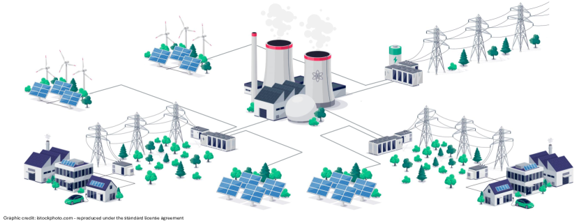
(a) Schematic of the grid configuration considered - one large synchronous generator coupled to many smaller IBRs.

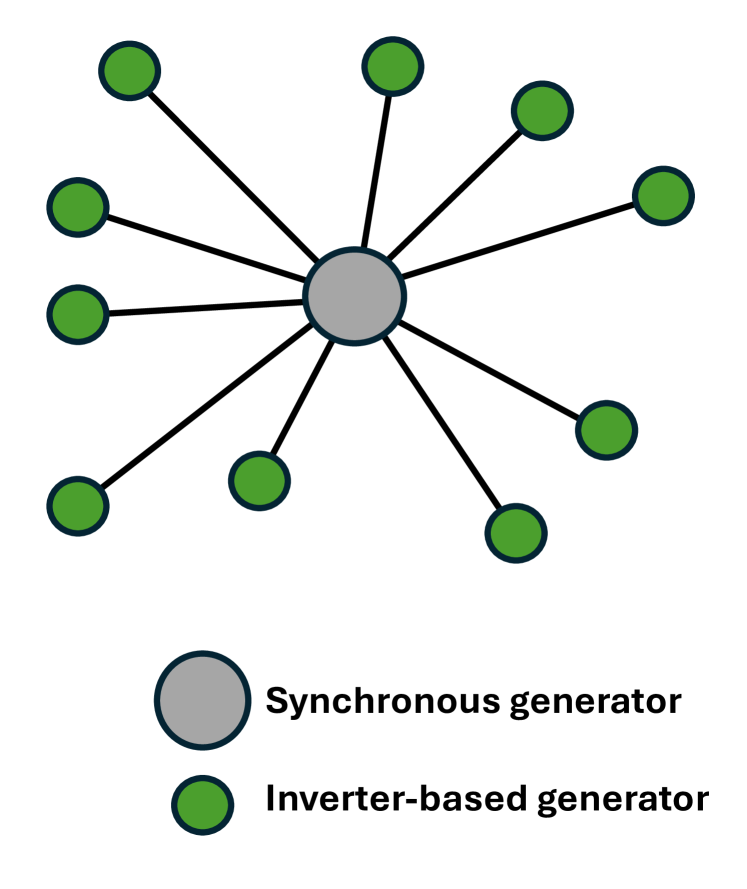
(b) Topological representation of the network considered, a so called ”hub and spokes” graph

Figure 1: Depiction of the studied network topology: A large synchronous generator is coupled to $n$ relatively smaller IBRs - even though the graphic here labels the largest generation unit as a nuclear plant, it could just as well be hydro or natural gas combined cycle unit.

An important assumption is that IBRs have negligible influence on one another, and that only their coupling with the large synchronous generator is significant. This assumption models the fact that in power grids dominated by a large capacity power station, it is likely that there are more transmission lines joining sections of the grid to the main generator than there are lines joining smaller generators to each other, forming a radial network [27]. This is intuitive because generators with larger inertia are most commonly synonymous with larger generation capacities, thus more transmission circuits are required to transfer that power to the loads, which offer more transfer capability and subsequently stronger coupling [43]. We therefore model the grid as having a “hub-and-spokes” topology, with the large synchronous generator at the center. In terms of our mathematical model, this corresponds to setting $K_{ij}=0$ if $i\neq 1$ and $j\neq 1.$ This topology is illustrated in Figure 1.

This topology for the power grid is comparable to those in geographic regions which have a large nuclear or hydro power plant, as well as high shares of IBRs. Since many regions fit this description, this particular topology is of significant interest. For example, in the Western Interconnection of the North American power grid, the Palo Verde Nuclear power plant (SG-based), is the largest nuclear energy facility in the United States and serves as the central element of frequency stability in the region [48, 39]. The large number of distributed generators in the Southwest desert region including Southern California, Arizona, and New Mexico, mainly utility-scale solar power plants and roof top solar panels, form a similar topology. Similarly, the Pacific Northwest and New England regions of the North American power grid have large hydro power plants with synchronous generators. These units are accompanied by larger numbers of IBRs, smaller distributed generation and large solar and wind power plants, at times forming a similar topology to that depicted in Figure 1. [23, 16] It is also interesting to note that this particular grid topology is similar to the topology of the power grid that the National Aeronautics and Space Administration (NASA) is considering for the Lunar power grid, [10, 11], and therefore could serve as the basis for this unique application.

Additionally, we make the simplifying assumptions that $\theta_{ij}=\pi/2$ for all $i,j$, which corresponds to the admittances being purely imaginary. This assumption is common, and is known as the lossless network assumption [37]. In fact, this is not far from the truth - in an example 39-bus network, which is a standard benchmark, after performing Kron reduction to reduce the network to only dynamically relevant nodes, the average value of $\theta_{ij}$ was $1.63$ with a standard deviation of $.07$, which represents a $3.7\%$ relative deviation from $\pi/2$.

Finally, we choose to let the phase of generator $n$ serve as a reference phase, against which all other phases are measured. This allows for the convenient property that a frequency-synchronized state will correspond to a fixed point of the dynamical network. We accomplish this with the simple coordinate transformation $\delta_{i}\to\delta_{i}-\delta_{n}$ for each $i$. Note that this implies that $\delta_{n}=\dot{\delta}_{n}=0,$ effectively decreasing the order of our network by $1$.

These simplifying assumptions allow the governing equations of motion to be written as:

$$\dot{\delta}_{i} =\omega_{i}-\omega_{n}\text{, }\hskip 10.0pti=1,\ldots,n$$ (2)

$$\dot{\omega}_{1} =\frac{\omega_{R}}{2H_{1}}\left(-D_{1}\omega_{1}+A_{1}-\sum_{j=2}^{n}K_{1j}\sin(\delta_{1}-\delta_{j})\right)$$

$$\dot{\omega}_{i} =\frac{\omega_{R}}{2H_{i}}\left(-D_{i}\omega_{i}+A_{i}-K_{i1}\sin(\delta_{i}-\delta_{1})\right)\text{, }\hskip 2.0pti\neq 1.$$

2.1 Mechanical Analog

To gain some intuition for equations (2), we describe a mechanical network which is governed by equations which are equivalent to (1). We note that a very similar mechanical model was studied in [19] and [15] in the context of Kuramoto oscillators representing networks of coupled inertialess power inverters. This mechanical model is illustrated in Figure 2.

Consider a collection of $n$ masses $m_{1},\ldots,m_{n}$ confined to move along a circular track of radius $R=1$. Let $\delta_{i}$ denote the angular displacement of mass $i$, and let $\omega_{i}=\frac{d\delta_{i}}{dt}$. Each mass $m_{i}$ is coupled to every other mass $m_{j}$ by an idealized spring which obeys Hooke’s law with spring constant $K_{ij}$. To be precise, we also must assume that these idealized springs have an equilibrium length of $0$, so that the force between $m_{1}$ and $m_{i}$ is always attractive. We further assume that the masses never collide, in order for the system to more closely resemble the electrical model.

Now, suppose each mass is subject to a constant propulsive force of $A_{i}$ which acts in the positive (counterclockwise) direction. Finally, suppose the whole network is subject to some type of fluid resistance damping, which is proportional to the angular velocity, so that the total damping force on mass $i$ is given by $-D_{i}\omega_{i}$. The varying values of $D_{i}$ could be due to different cross sectional areas, for example.

The power system model presented in Section 2 is analogous to this mechanical model in the case with $m_{1}\gg m_{i}$ for $i>1$, and when $K_{ij}\approx 0$ if $i,j\neq 1$.

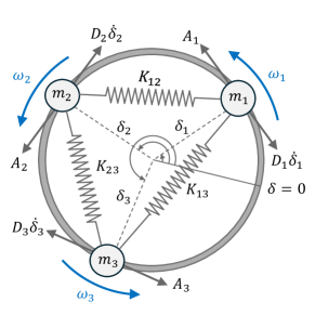
Figure 2: A mechanical network analogous to the power grid model described in Section 2: this system is considered in a stable synchronized state when $\omega_{1}=\omega_{2}=\omega_{3}$.

We now derive the equations of motion for the system depicted in Figure 2. First, one can compute that the distance between mass $i$ and $j$ is given by $2\sin\left(\frac{\delta_{i}-\delta_{j}}{2}\right)$, so that the spring force between $i$ and $j$ is given by $-2K_{ij}\sin\left(\frac{\delta_{i}-\delta_{j}}{2}\right)$. However, since the carts are confined to move on a circular track, only the component of this force tangent to the circle contributes to the cart’s acceleration. A small trigonometric calculation reveals that the tangential component of the force is given by $-2K_{ij}\sin\left(\frac{\delta_{i}-\delta_{j}}{2}\right)\cos\left(\frac{\delta_{i}-\delta_{j}}{2}\right)=-K_{ij}\sin\left(\delta_{i}-\delta_{j}\right)$. The other forces $A_{i}$ and $-D_{i}\dot{\delta}_{i}$ act on $m_{i}$ in the tangential direction by assumption. Newton’s second law then gives that:

$$m_{i}\ddot{\delta_{i}}=A_{i}-D_{i}\dot{\delta}_{i}-\sum_{j\neq i}K_{ij}\sin(\delta_{i}-\delta_{j}).$$ (3)

Now, we make the assumption that $m_{1}\gg m_{i}$ for all $i>1$ and $K_{ij}\approx 0$ for $i,j\neq 1$ in order to agree with the power grid model we are studying. This corresponds to the assumption that the grid is dominated by a single oscillator with significant inertia (the synchronous generator) which is coupled strongly to several smaller oscillators (the IBRs), and that the coupling between the small oscillators is negligible. Writing $\dot{\delta}_{i}=\omega_{i}$, equation 3 can be rewritten as the system:

$$\dot{\delta}_{i} =\omega_{i}$$ (4)

$$\dot{\omega}_{1} =(m_{1})^{-1}\left(-D_{1}\omega_{1}+A_{1}-\sum_{j=2}^{n}K_{1j}\sin(\delta_{1}-\delta_{j})\right)$$

$$\dot{\omega}_{i} =(m_{i})^{-1}\left(-D_{i}\omega_{i}+A_{i}-K_{j1}\sin(\delta_{j}-\delta_{1})\right)\hskip 2.0pt\text{for }i\neq 1.$$

The clear similarities between equations (4) and (2) show that this mechanical model can be used to represent the synchronization properties of our swing equation. Figure 3 illustrates a numerical simulation of equations (4) using the Differential Equations package in Julia. The damping, propulsive force, mass, and coupling of each oscillator, as well as their initial phase and frequency, are randomly chosen within physically relevant ranges. The system is then numerically integrated using the Tsitouras Runge-Kutta/Rosenbrock-W methods [40] with a relative tolerance of $10^{-9}$ and is run for enough time to allow the system to synchronize. At time $t=0,$ the system is subjected to a sudden frequency disturbance which throws all the masses out of synchronization. Notice that within a few seconds of the disturbance, the masses re-synchronize. This shows that for the given parameters of the problem (listed in the appendix) the synchronized state is stable.

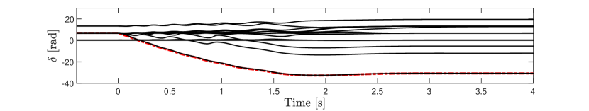
(a) Angular position, relative to the reference mass $n$

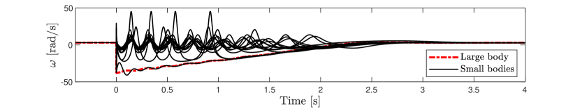
(b) Frequency

Figure 3: The phase and frequency response of the mechanical network depicted in Figure 2 with $n=15$. Masses are started with random initial conditions after a period of initial transience, but quickly settle to the predicted value of $\omega_{sync}$ (that is the pre-disturbance velocity all bodies). At time $t=0$, the oscillators are subjected to a sudden impulsive frequency drop. After roughly 4 seconds, the masses re-synchronize at $\omega_{sync}$. Details of the simulation can be found in the appendix.

2.2 Model Reduction

As a next step in our treatment of the swing equations (2), we take advantage of the fact that the IBRs have extremely small inertias, $H_{i}\approx 0$ for $i>1$, in order to reduce the order of the swing equations (2) and obtain a simpler system with equivalent long term behavior. In general, studying the behavior of systems of differential equations which have a small parameter multiplying their highest-order derivatives involves an intricate analysis using boundary layer theory and matched asymptotics [5]. However, in our case, we are only concerned with the long time behavior of the system - whether or not the system will eventually synchronize. The tool that enables us to do so is Tikhonov’s Reduction Theorem of singular perturbation theory. We refer the reader to [26] for an excellent introduction to the use of this tool.

We model the assumption that the IBRs have negligible inertia by writing $H_{i}=\epsilon h_{i},$ where $h_{i}$ is $\mathcal{O}(1)$ and $\epsilon\ll 1.$ Tikhonov’s Theorem [26] then guarantees that on time scales much larger than $\epsilon\log\epsilon,$ the solution to (2) will tend towards the solutions of the so called “degenerate system,” given by

$$\dot{\delta}_{i}= \omega_{i}-\omega_{n}\hskip 10.0pti=1,\ldots,n-1$$ (5)

$$\dot{\omega}_{1}= \frac{\omega_{R}}{2H_{1}}\left(-D_{1}\omega_{1}+A_{1}-\sum_{\begin{subarray}{c}j=2\end{subarray}}^{n}K_{1j}\sin(\delta_{1}-\delta_{j})\right)$$ (6)

$$\omega_{i}= \frac{1}{D_{i}}\left(A_{i}-K_{i1}\sin(\delta_{i}-\delta_{1})\right)\hskip 10.0pti=2,\ldots,n.$$ (7)

Notice that we have reduced the original $2n-1$ differential equations to $n$ differential equations equations and $n-1$ algebraic equations. Equations (5)-(7) constitute the primary model that we study in the remainder of this work.

2.3 A Note on Units

Note that all of the parameters in equations (5)-(7) have dimensions of power, other than the damping $D_{i}$ which has dimensions of energy, and $\omega_{R}$ which has dimensions of frequency. For the remainder of this work, we use the following conventions for the units used for the parameters in equations (5)-(7) . We set $\omega_{R}=377\frac{\text{rad}}{\text{sec}}\approx 60\text{Hz},$ the grid frequency in the United States. For the other parameters, we use the per-unit system, with 1 $\text{pu}=100\text{MW}.$ We then take the power generated by the large synchronous generator to be in the range $5\leq A_{1}\leq 15$, comparable to a large nuclear power plant. The smaller generators are taken in the range $.25\leq A_{i}\leq 5,$ corresponding to many large-scale solar projects. We take the inertia constant $H_{1}$ to be in the range $4-8\text{ pu},$ while inertia constants for the IBRs are taken to be on the order $10^{-4}\text{ pu}.$ Damping values $D_{i}$ are taken in the range $0.001-0.01\text{ pu}\cdot\text{sec}$ for all generators. Coupling constants $K_{1i},$ which correspond more or less to the transfer admittances of the lines joining the generators, are taken in the range $5-15\text{p.u.}.$ For all of the simulations that follow, parameters are randomly assigned, within the above physically relavent ranges. We point out, however, that all of our subsequent mathematical analysis is valid for general values of the parameters.

3 Existence of Synchronized Modes

In this secion and the next, we discuss our main results on synchronization. By construction, a synchronized mode of system (5)-(7) is a fixed point for the system in which $\omega_{i}=\omega_{n}$ for each $i$. We therefore begin our analysis by looking for fixed points of the system (5)-(7).

Notice that in order for the left hand side of equation (5) to be equal to $0$, it must be the case that $\omega_{i}=\omega_{n}$ for all $i$. Therefore the only fixed points supported by system (5)-(7) are frequency synchronized states. It is the existence and stability of these fixed points in which we are interested.

Proposition 1 (Synchronization Frequency).

If the generators governed by equations (5)-(7) synchronize, the synchronization frequency must be given by

$$\omega_{sync}=\frac{\sum_{j=1}^{n}A_{j}}{\sum_{j=1}^{n}D_{j}}.$$

Proof.

To begin, note that equation (7) can be rewritten as $D_{i}\omega_{i}-A_{i}=-K_{i1}\sin(\delta_{i}-\delta_{1}).$ Now, equation (5) implies that at a fixed point, all of the frequencies are identical, so we must have

$$D_{i}\omega_{1}-A_{i} =-K_{i1}\sin(\delta_{i}-\delta_{1})$$

$$=K_{1i}\sin(\delta_{1}-\delta_{i}),$$

where we have used that the coupling is symmetric, $K_{1i}=K_{i1}.$ Therefore, at a fixed point, we can rewrite equation (6) as:

$$0 =-D_{1}\omega_{1}+A_{1}-\sum_{j=2}^{n}K_{1j}\sin(\delta_{1}-\delta_{2})$$

$$0 =-D_{1}\omega_{1}+A_{1}-\sum_{j=2}^{n}(D_{i}\omega_{1}-A_{i})$$

$$0 =-\left(\sum_{j=1}^{n}D_{i}\right)\omega_{1}+\sum_{j=1}^{n}A_{j}$$

which implies that

$$\omega_{1}=\omega_{sync}=\frac{\sum_{j=1}^{n}A_{j}}{\sum_{j=1}^{n}D_{j}}$$ (8)

as desired.

∎

We note that the result of Proposition 1 agrees with Theorem 2 found in [15] in the context of an all-IBR network. Proposition 1 implies that maintaining a constant stable grid frequency requires balancing the total network injected power ($\sum A_{j}$) with total network damping ($\sum D_{j}$). In the United States, for example, this quantity must be held as closely as possible to $\omega_{sync}=377\frac{\text{rad}}{\text{sec}}$ ($60\text{Hz}$). In the next proposition, we derive an important necessary condition for the existence of synchronized modes.

Proposition 2 (Necessary Condition for Synchronization).

The reduced swing equations (5) - (7) support fixed points (and therefore, synchronization) only when

$$K_{i1}\geq\left|D_{i}\omega_{sync}-A_{i}\right|$$ (9)

for each $i>1.$

Proof.

Note that at a fixed point, when $\omega_{1}=\ldots=\omega_{n}=\omega_{sync},$ equation (7) implies that:

$$K_{i1}\sin(\delta_{1}-\delta_{i})=D_{i}\omega_{sync}-A_{i}$$ (10)

for $i>1.$ Because $\left|\sin(\delta_{1}-\delta_{i})\right|\leq 1$ for all values of the argument, we immediately find that the existence of a fixed point requires that

$$K_{i1}\geq\left|{D_{i}\omega_{sync}-A_{i}}\right|,$$

as desired. ∎

Having easily established the necessary condition (9), we now use equation (10) to find the phases $\delta_{i}$ associated with a fixed point. Plugging in $\delta_{n}$ into (10) and recalling that $\delta_{n}=0,$ we find that:

$$\sin(\delta_{1})=\frac{1}{K_{n1}}\left(D_{n}\omega_{sync}-A_{n}\right).$$ (11)

Let $\sin^{-1}$ denote the principal branch of the arcsine function, with values between $-\pi/2$ and $\pi/2.$ Then we can rewrite equation (11) as:

$$\delta_{1}=(-1)^{k}\sin^{-1}\left(\frac{D_{n}\omega_{sync}-A_{n}}{K_{n1}}\right)+k\pi$$ (12)

for $k\in\mathbb{Z}$. In fact, it suffices to consider just $k=0$ and $k=1$, since $\delta_{1}\in[0,2\pi)$. Now, to simplify notation, define $\mu_{i}:=\frac{D_{i}\omega_{sync}-A_{i}}{K_{i1}}$. Equation (10) can then be rewritten as

$$\begin{split}\sin(\delta_{1}-\delta_{i})&=\mu_{i}\\ \delta_{1}-\delta_{i}&=(-1)^{j}\sin^{-1}(\mu_{i})+j\pi\\ \delta_{i}&=\delta_{1}+(-1)^{j+1}\sin^{-1}(\mu_{i})-j\pi\quad\text{for }j=0,1\end{split}$$ (13)

Together, equations (12), (13), and (8) determine the locations of all of the fixed points of the reduced swing equations (5)-(7). Note that this implies the existence of $2^{2n-2}$ total fixed points. Finally, note that we have not yet found any information about the stability of the synchronized modes, only the existence. We address the question of stability next, in Section 4.

4 Stability of Synchronized Modes

We now derive an approximate sufficient condition for the local stability of a frequency synchronized mode. We proceed by linearizing the model (5)-(7) and finding an approximate condition for all of the eigenvalues to have negative real part in the neighborhood of one of the frequency-synchronized modes computed in Section 3. Local exponential stability then follows by the Hartman-Grobman theorem [20, 18].

The vector field defined by equations (5)-(7) is given by the mapping

$$F:\mathbb{R}^{n} \to \mathbb{R}^{n}$$

$$(\delta_{1},\ldots,\delta_{n-1},\omega_{1}) \mapsto \left(\omega_{1}-\omega_{n},\ldots,\omega_{n-1}-\omega_{n},\dot{\omega}_{1}\right),$$

where $\omega_{i>1}$ is given by $\omega_{i}=\frac{1}{D_{i}}\left(A_{i}-K_{i1}\sin(\delta_{i}-\delta_{1})\right),$ $\dot{\omega}_{1}=\frac{\omega_{R}}{2H_{1}}\left(-D_{1}\omega_{1}+A_{1}-\sum_{\begin{subarray}{c}j=2\end{subarray}}^{n}K_{1j}\sin(\delta_{1}-\delta_{j})\right)$, and $\delta_{n}$ is understood to be constantly $0$. Then the Jacobian of $F$ at $(\delta_{1},\ldots,\delta_{n-1},\omega_{1})$ is given by:

$$J=\left[\begin{matrix}-\alpha_{1}&0&0&\cdots&0&1\\ \alpha_{2}-\alpha_{1}&-\alpha_{2}&0&\cdots&0&0\\ \alpha_{3}-\alpha_{1}&0&-\alpha_{3}&\cdots&0&0\\ \vdots&&&\ddots&\vdots&\vdots\\ \alpha_{n-1}-\alpha_{1}&0&0&\cdots&-\alpha_{n-1}&0\\ -\sum_{j=2}^{n}\beta_{j}&\beta_{2}&\beta_{3}&\cdots&\beta_{n-1}&\eta\end{matrix}\right]$$ (14)

where $\alpha_{1}=\frac{K_{n1}}{D_{n}}\cos(\delta_{1})$, $\alpha_{j}=\frac{K_{j1}}{D_{j}}\cos(\delta_{1}-\delta_{j})$ for $j>1$, and $\beta_{j}=\frac{K_{1j}\omega_{R}}{2H_{1}}\cos(\delta_{1}-\delta_{j})$, and $\eta=\frac{-D_{1}\omega_{R}}{2H_{1}}$.

Now, stability at a fixed point requires that all of the eigenvalues of $J$ have negative real part at that point. Our strategy in this section is to find an approximation for the eigenvalues of matrix $J$ at a fixed point given by equations (12) and (13). This approximation then can be used to find a condition for the eigenvalues of $J$ to have negative real part.

The next proposition first proves the existence of the an attractive fixed point, which establishes the existence of a stable synchronized mode.

Proposition 3.

Suppose that the necessary condition (9) is satisfied. Then for sufficiently large values of $K_{n1}$, exactly one of the synchronized modes found in equations (8), (12), and (13) is locally stable.

Proof.

First, note that the Jacobian $J$ is almost a lower triangular matrix, other than the entry $1$ in position $(1,n)$. Let $L$ denote the lower triangular matrix given by removing this undesirable entry from $J$. The eigenvalues of $L$ are given by the diagonal elements, $-\alpha_{1}$, $-\alpha_{2},\ldots,-\alpha_{n-1}$ and $\eta$. Recall that there are $2$ values of $\delta_{1}$ which give rise to a fixed point, and for each of these there correspond $2$ different values of $\delta_{i}$ for each $i$, and that each of these values essentially differs by $\pi$ (see equations (12) and (13) ). It is therefore possible to choose $\delta_{1}$ and each $\delta_{i}$ so that $-\alpha_{1}$ and $\alpha_{i}$ for $1<i\leq n-1$ are all negative. Call this fixed point $\delta^{*}$. Note that this is the only fixed point which will have $\cos(\delta_{1}-\delta_{i})>0$ for each $i$, which is necessary for $L$ to have all negative elements on the diagonal. Hence, $\delta^{*}$ is the only fixed point at which $L$ has all negative eigenvalues. We next argue that the eigenvalues of $J$ cannot differ too much from the eigenvalues of $L$, which will show that $\delta^{*}$ is a stable fixed point of the reduced swing equations.

Next, factor out $\left|\alpha_{1}\right|$ from $J$, and let $J=\left|\alpha_{1}\right|\tilde{J}$. Note that $J$ has all negative eigenvalues if and only if $\tilde{J}$ does as well. We write $\tilde{J}$ in block matrix form as:

$$\tilde{J}=\left[\begin{matrix}-1&\boldsymbol{0}^{T}&\epsilon\\ \boldsymbol{\alpha}&\Lambda&\boldsymbol{0}\\ \gamma&\boldsymbol{\beta}^{T}&\lambda_{n}\end{matrix}\right]$$

where $\boldsymbol{0}$ is the $0$ vector of size $n-2$ , $\epsilon=1/\left|\alpha_{1}\right|$, $\boldsymbol{\alpha}$ and $\boldsymbol{\beta}$ are vectors of length $n-2$, and $\gamma$ and $\lambda_{n}$ are scalars. Notice that $\tilde{J}$ differs from a lower triangular matrix by an entry of $\epsilon$ in position $(1,n)$ At $\delta^{*}$, all the diagonal entries of $\tilde{J}$ are negative. Eigenvalues depend continuously on the entries of a matrix. (This fact follows from the continuity of the determinant and the fact that the roots of polynomials depend continuously on their coefficients). Hence, for $\epsilon$ sufficiently small, the eigenvalues of $\tilde{J}$ are all negative. It follows that for $K_{n1}$ sufficiently large, all of eigenvalues of $J(\delta^{*})$ are negative, and hence $\delta^{*}$ is locally stable.

∎

Note that the proof could have been carried out by factoring out $\left|\alpha_{i}\right|$ for any $i$, and hence a slight strengthening of the proposition would be to state that if any of the $K_{i1}$ is sufficiently large, then $\delta^{*}$ is locally stable.

In the next series of results, we strengthen the result of Proposition 3 by deriving a sharper sufficient condition for local stability of the fixed point $\delta^{*}$.

Proposition 4.

Let $L$ be the lower triangular part of matrix $J$ given in equation (14), and let $E$ be the matrix of all zeros except for a $1$ in position $(1,n)$. Suppose that all of the eigenvalues of $L$ are distinct, and let $\lambda_{j}(0)$ denote the $j^{th}$ eigenvalue of matrix $L$, given by $L_{jj}$, and let $\lambda_{j}(s)$ denote the corresponding eigenvalue of the matrix $L+sE.$ Then $\lambda_{j}$ is analytic in a neighborhood of $s=0$, and

$$\lambda_{j}^{\prime}(0)=\frac{(w_{j})_{1}(v_{j})_{n}}{w_{j}\cdot v_{j}},$$ (15)

where $v_{j}$ and $w_{j}$ denote the right and left eigenvectors associated with $\lambda_{j}(0),$ respectively, and $(w_{j})_{1}$ and $(v_{j})_{n}$ denote their $1^{st}$ and $n^{th}$ components, respectively.

Proof.

The analyticity of $\lambda_{j}(s)$ in a neighborhood of $s=0$ follows from the analyticity of the function $s\mapsto L+sE$ and the Implicit Function Theorem, provided that the mulitplicity of each eigenvalue is $1$. We can therefore implicitly differentiate the expression $(L+sE)v_{j}(s)=\lambda_{j}(s)v_{j}(s)$ to find that

$$Ev_{j}(s)+(L+sE)v_{j}^{\prime}(s)=\lambda_{j}^{\prime}(s)v_{j}(s)+\lambda_{j}(s)v_{j}^{\prime}(s).$$

For the rest of the proof we suppress the argument $s$ to simplify the notation. Now, left multiply both sides of the above equation by the left eigenvalue $w_{j}^{T}$:

$$w_{j}^{T}Ev_{j}+w_{j}^{T}(L+sE)v_{j}^{\prime} =w_{j}^{T}\lambda_{j}^{\prime}v_{j}+w_{j}^{T}\lambda_{j}v_{j}^{\prime}$$

$$w_{j}^{T}Ev_{j}+w_{j}^{T}\lambda_{j}v_{j}^{\prime} =w_{j}^{T}\lambda_{j}^{\prime}v_{j}+w_{j}^{T}\lambda_{j}v_{j}^{\prime}$$

$$w_{j}^{T}Ev_{j} =w_{j}^{T}\lambda_{j}^{\prime}v_{j}$$

from which it follows that

$$\lambda_{j}^{\prime}(0)=\frac{w_{j}^{T}Ev_{j}}{w_{j}^{T}v_{j}}.$$

Now simply compute that $w_{j}^{T}Ev_{j}=(w_{j})_{1}(v_{j})_{n}$ and the result follows.

∎

We will use Proposition 4 together with Taylor’s Theorem estimate the eigenvalues of the Jacobian $J$. Note that the eigenvalues of $J$ correspond to $\lambda_{i}(1).$ Taylor’s Theorem gives us that $\lambda_{i}(1)\approx\lambda_{i}(0)+\lambda^{\prime}_{i}(0),$ so the eigenvalues of $J$ are approximately given by $\lambda_{j}(0)+\frac{(w_{j})_{1}(v_{j})_{n}}{w_{j}\cdot v_{j}},$ where $\lambda_{j}(0)$ is exactly the $j^{th}$ diagonal element of $J$. Therefore, to approximate the eigenvalues of $J,$ all we need is to compute the left and right eigenvectors of the lower triangular part of $J,$ which we continue to denote $L$.

Let $e_{i}$ denote the $i^{th}$ standard basis vector of $\mathbb{R}^{n}.$ Recall that $\delta^{*}$ represents the fixed point at which $\cos(\delta_{1}-\delta_{i})>0$ for each $i>1$. Then one can compute that at $\delta^{*}$, the right eigenvectors of $L$ associated with eigenvalue $L_{ii}$ are given by:

$$\sum_{i=1}^{n-1}e_{i}+\frac{K_{n1}D_{n}\omega_{R}\sqrt{1-\mu_{n}^{2}}}{2H_{1}K_{n1}\sqrt{1-\mu_{n}^{2}}-D_{1}D_{n}\omega_{R}}e_{n} i=1,$$ for (16)

$$e_{i}-\frac{K_{i1}D_{i}\omega_{R}\sqrt{1-\mu_{i}^{2}}}{2H_{1}K_{i1}\sqrt{1-\mu_{i}^{2}}-D_{1}D_{i}\omega_{R}}e_{n} 1<i<n,$$ for

$$e_{n} i=n$$ for

where, as before, $\mu_{i}=\frac{D_{i}\omega_{sync}-A_{i}}{K_{1i}}$. Note that any scalar multiple of these eigenvectors is again an eigenvector, but this particular scaling will prove convenient. Similarly, one can compute that the left eigenvectors of $L$ associated with eigenvalue $L_{ii}$ are given by

$$e_{1}^{T} i=1,$$ for

$$e_{i}^{T}-e_{1}^{T} 1<i<n,$$ for

$$\frac{1}{\alpha_{1}+\eta}\left(\sum_{i=2}^{n-1}\frac{\beta_{i}(\alpha_{i}-\alpha_{1})}{\alpha_{i}+\eta}-\sum_{i=2}^{n}\beta_{i}\right)e_{1}^{T}+$$

$$\cdots+\sum_{i=2}^{n-1}\left(\frac{\beta_{i}}{\alpha_{i}+\eta}e_{i}^{T}\right)+e_{n}^{T} i=n$$ for

where $\alpha_{i},$ $\beta_{i},$ and $\eta$ are as defined just below equation (14).

Having computed the eigenvectors of the lower triangular part of $J$, we are now in position to use equation (15) to approximate the eigenvalues of $J$. Using Taylor’s formula, we have

$$\lambda_{j}(1)\approx\lambda_{j}(0)+\lambda^{\prime}_{j}(0),$$

assuming that $\lambda_{j}(s)$ is analytic for $s\in[0,1].$ Finally, we are able to state the following claim.

Claim 5.

Suppose that the functions $\lambda_{j}(s)$ are analytic on the whole interval $[0,1].$ Then eigenvalues of $J$ at the fixed point $\delta^{*}$ are approximately given by

$$\lambda_{1}\approx-K_{n1}\sqrt{1-\mu_{n}^{2}}\left(\frac{1}{D_{n}}+\frac{D_{n}\omega_{R}}{2H_{1}K_{n1}\sqrt{1-\mu_{i}^{2}}-D_{1}D_{n}}\right)$$ (17)

$$\lambda_{i}\approx-K_{i1}\sqrt{1-\mu_{i}^{2}}\left(\frac{1}{D_{i}}+\frac{D_{i}\omega_{R}}{2H_{1}K_{i1}\sqrt{1-\mu_{i}^{2}}-D_{1}D_{i}}\right)$$

$$\text{for }\hskip 5.0pti=2,\ldots,n-1\text{, and}$$

$$\lambda_{n}\approx\frac{-\omega_{R}}{2H_{1}}\sum_{i=1}^{n}D_{i}.$$

Assuming for a moment the correctness of the approximation given in Claim 5, we are able to obtain the following stability condition.

Proposition 6.

Suppose that the eigenvalues of $J$ are given by the expressions in (17). Then the eigenvalues have negative real part if:

$$K_{i1}^{2}>\left(\frac{D_{1}D_{i}\omega_{R}}{2H_{1}}\right)^{2}+(D_{i}\omega_{R}-A_{i})^{2}$$ (18)

for each $i=2,\ldots,n$. In this case, the fixed point $\delta^{*}$ is locally stable.

Before beginning the proof of Proposition 6, it is worth noting how inequality (18) compares with the necessary condition (9). The main difference is the addition of the term $((D_{1}D_{i}\omega_{R})/(2H_{1}))^{2},$ which in practice is a very small quantity: the damping value $D_{1}$ for a large synchronous generator is likely on the order of $10^{-2},$ while the damping for an IBR is on the order of $10^{-5}$ for a grid following inverter and $10^{-1}$ for a grid forming inverter, whereas in $H_{1}$ is on the order of $10$ pu. Hence, inequality (18) differs from the necessary condition (9) by a quantity with a magnitude of roughly $10^{-3}$. Hence, in practice, the difference between our necessary and our approximate sufficient conditions is very small.

Proof.

Notice in expression (17) that the expression for $\lambda_{n}$ is always negative. Moreover, in the expressions for $\lambda_{i}$ for $i=1,\ldots,n-1$, the prefactor $-K_{i1}\sqrt{1-\mu_{i}^{2}}$ is negative, hence to ensure each eigenvalue is negative, all that is necessary is to force the expressions inside the parentheses to be positive. This can be done by requiring that

$$2H_{1}K_{i1}\sqrt{1-\mu_{i}^{2}}-D_{1}D_{i}>0.$$

Recalling that $\mu_{i}=(D_{1}\omega_{R}-A_{i})/K_{i1}$, and then rearranging the above expression for $K_{i1}$ quickly gives inequality (18). ∎

4.1 On the strength of eigenvalue approximation.

It is worth spending a moment addressing how good the approximation (17) is. First, assuming that $\lambda(s)$ is analytic on the entire interval $[0,1]$, Taylor’s Remainder Theorem gives that

$$\left|\lambda_{true}-\lambda_{appr}\right|\leq\max_{s\in[0,1]}\frac{\lambda^{\prime\prime}(s)}{2},$$

where again, $\lambda(s)$ denotes an eigenvalue of $L+sE,$ as in the proof of Proposition 4. One can even use equation 15 to compute an expression for $\lambda^{\prime\prime}(s)$ - however, explicitly evaluating the resulting expression depends on being able to compute the left and right eigenvectors $w(s)$ and $v(s)$ of $L+sE$ for each $s\in[0,1]$, which is indeed unwieldy. However, being able to do so would give precise bounds on the accuracy of the approximation (18), and will therefore be the object of future research.

In the absence of an analytic bound on the error in approximation (17), we turn to numerical approaches. In Figure 4, we compared the approximate eigenvalues (17) and the true eigenvalues of the matrix $J$. To generate the figure, 10,000 matrices were randomly generated in the form of $J$ using Julia, with parameters randomly chosen to be within physically relevant ranges. The matrices were size $10\times 10$, representing $n=10$ generators consisting of $1$ large generator and $9$ IBRs. For each matrix, the true eigenvalues of $J$ were computed and were compared to the approximate values (17). The average error between each true eigenvalue and the approximated eigenvalue was then computed. In Figure 4, we plot the error in our prediction against the minimum distance between the eigenvalues of $J$ on the horizontal axis - if the distance between two eigenvalues of $J$ gets very small, the error in our approximation tends to get worse. This reflects the fact that the functions $\lambda(s)$ are analytic only if no two eigenvalues of $L+sE$ are equal; hence, when the minimum distance between two eigenvalues is small, $\lambda(s)$ is close to a singularity, making matrix $L$ ill-conditioned, and therefore the error in approximation (17) tends to be larger. However, even so, note that the error in our approximation is almost always less than $10\%$, and quite often much less than $5\%$. In generating Figure 4, we omitted cases where the function $\lambda(s)$ is not analytic over the interval $[0,1]$; such cases are relatively rare, but in these cases approximation (17) breaks down.

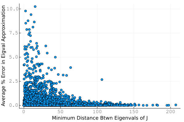
Figure 4: A comparison of the eigenvalue approximation (17) with the true eigenvalues of the matrix $J$: the error is fairly small, very often below 5%. Notice that the error tends to be larger when two eigenvalues of $J$ are very close to each other; in such cases, the matrix $J$ is ill-conditioned, and approximation (17) tends to be worse.

It is worth noting that there are other approaches to approximating the eigenvalues of $J$ which may also prove fruitful in future research. In particular, the Gerschgorin Circle Theorem [50] and the Bauer-Fike Theorem [12] both give rigorous bounds on how much the eigenvalues of $J$ can deviate from those of $L$. While these methods give precise results, we have found that the bounds that they give on the location of the eigenvalues are too coarse to guarantee the stability of the synchronized fixed point. This is why we have opted for our approximate approach, while less rigorous than one of these methods, we are able to derive much tighter conditions, albeit approximate ones. An object of future research will be to combine the rigour of these two aforementioned theorems with the tightness of our approximate bound.

5 Implications for Stability and Control of Modern Power Systems

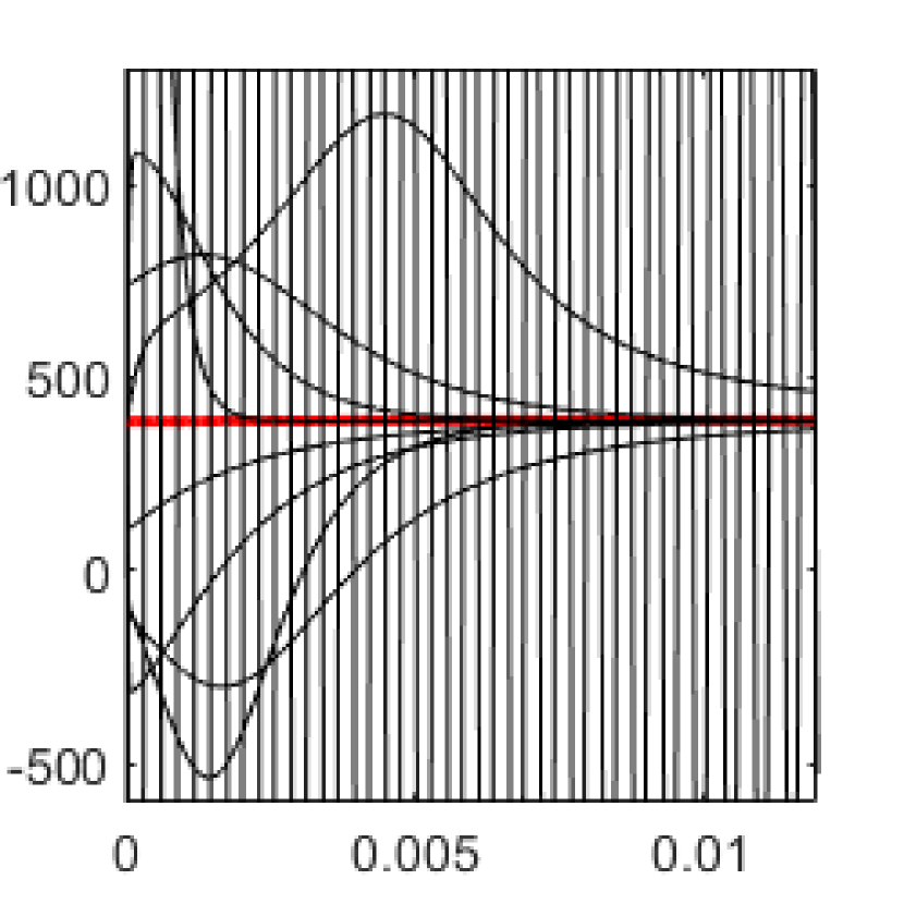
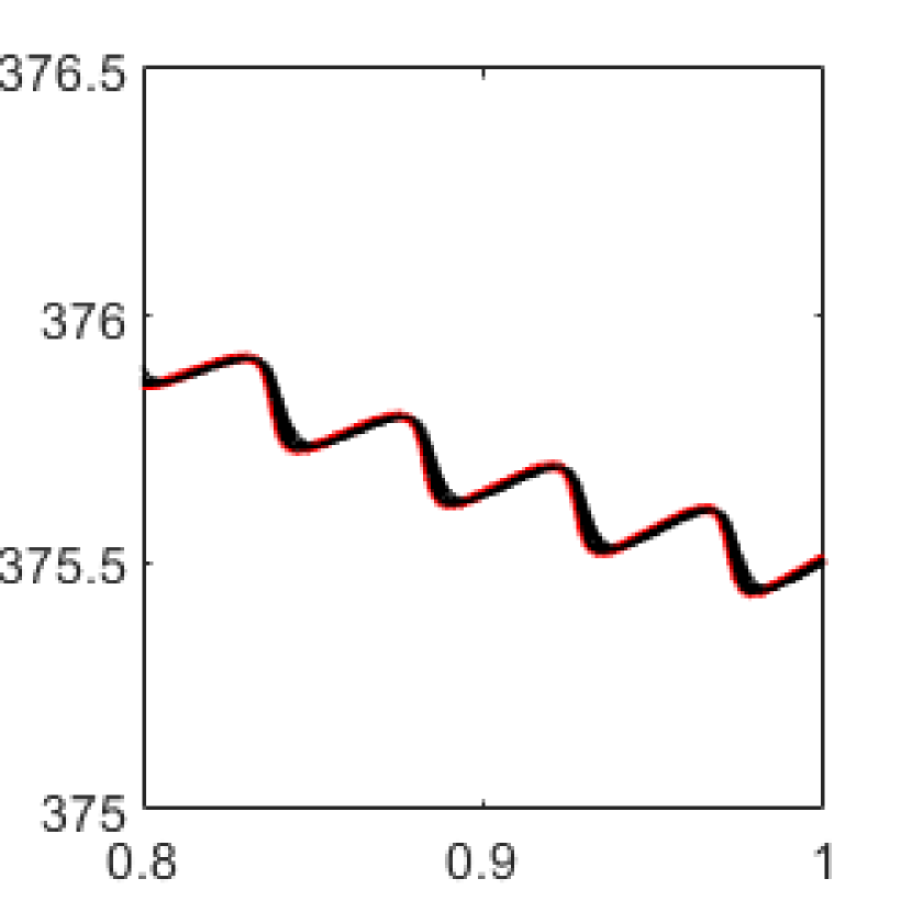
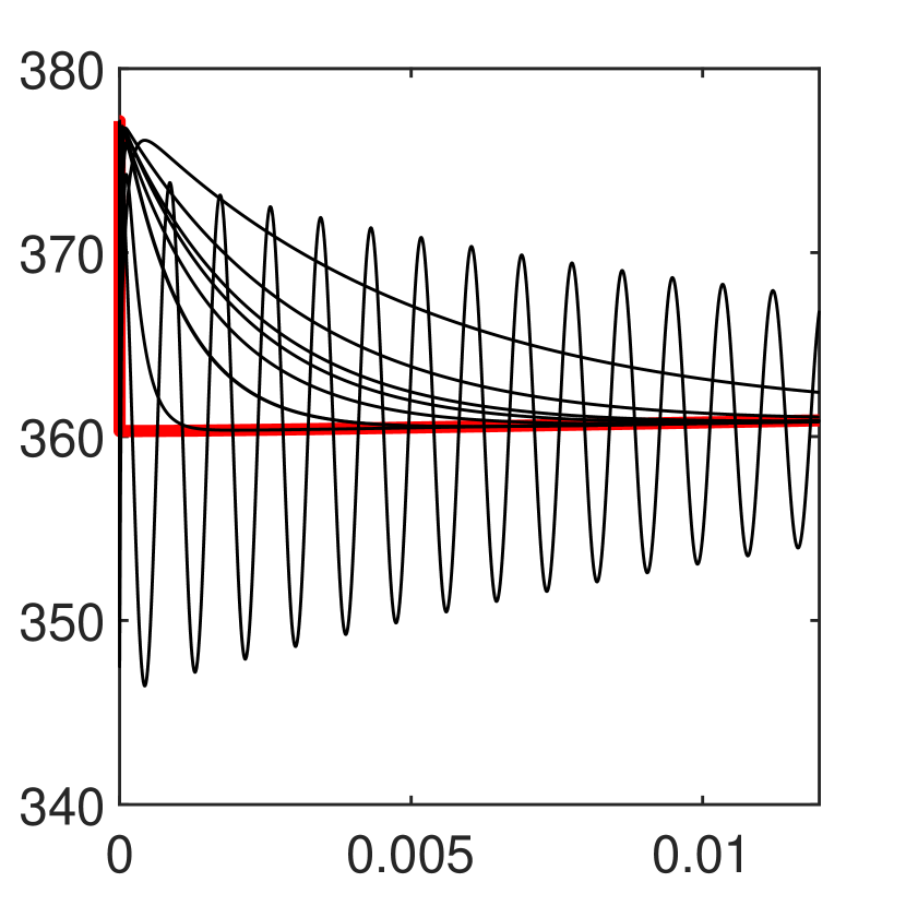
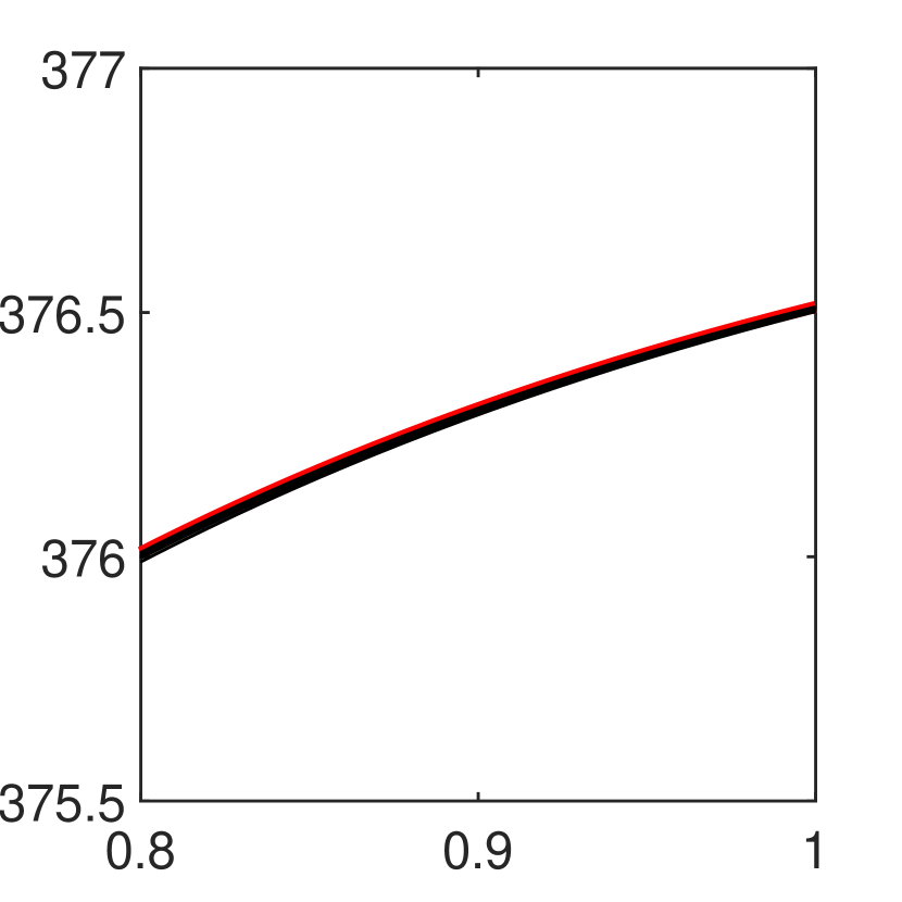
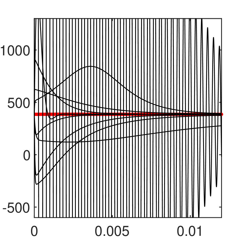
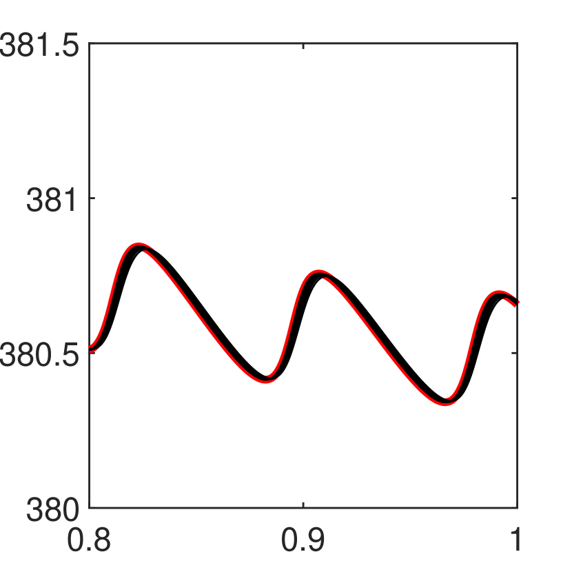
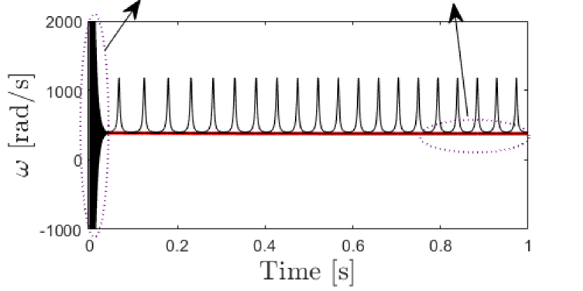
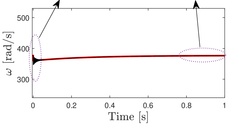
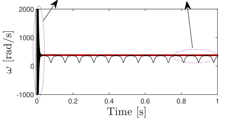
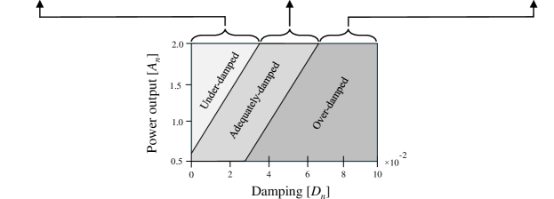
Figure 5: The central graphic in the $A_{n}$-$D_{n}$ plane shows the region of parameter space corresponding to the necessary condition, inequality (9). The three graphs show the result of numerical simulation of the swing equations (1) with $10$ generators, in the cases where generator $10$ is under-damped, over-damped, and adequately damped, respectively. Notice that both the under-damped scenarios cause generator $10$ to enter into wild oscillations, which in turn pull the rest of the network out of sync. In the adequately damped case, notice that the IBRs quickly synchronize with the SG, and the whole system then steadily increases towards the desired synchronization frequency of $377\text{ rad}/\text{sec}$.

Taken together, the conditions found in this paper imply that stable operation of a strongly heterogeneous power grid is determined by the relationship between the power supplied by a given generator $A_{i}$, the damping value of this generator $D_{i}$, and the coupling $K_{i1}$. Generally, the coupling values $K_{i1}$ are determined by the admittance of the transmission lines connecting the small generators to the large one, and therefore from the perspective of a grid operator are seen as being more or less given. By contrast, the variables $A_{i}$ and $D_{i}$ are both potentially under the control of the grid operator, and thus conditions (9) and (18) have practical implications for the stable operation of power systems. In what follows, we wish to emphasize three practical implications of these results for power systems engineering.

First, inequality (9) has implications about when it is appropriate for an IBR to interface with the rest of the grid using a GFL versus a GFM. In particular, it is has been shown that when modelling inverter based resources as a second order dynamical system, the primary difference between GFLs and GFMs is that GFLs have $D_{i}\approx 0$, whereas GFMs can be operated with $D_{i}>0$[46, 24, 25]. Inequality (9) suggests that GFLs should only be implemented on generators where the power output $A_{i}$ satisfies $A_{i}\leq K_{i1}$; a generator with next to no damping ($D_{i}\approx 0$) can only interact with the grid in a stable way if its power output is less than the coupling value $K_{i1}$. For a generator with $A_{i}>K_{i1}$ to interact with the grid in a manner that supports synchronization requires sufficient damping be added so that the inequality (18) be satisfied. This implies that IBRs producing large power outputs should be outfitted with GFMs rather than GFLs to support frequency synchronization in the grid.

A second practical consequence of inequality (9) is that there are two ways for an IBR to cause the grid to lose stability - either by being over-damped or by being under-damped. As illustrated in Figure 5, both scenarios can have equally dramatic effects on overall frequency stability. The data in this figure was generated by simulating equations (1) in Julia, using $n=10$ generators, whose parameters are given in the appendix. In each subfigure, the damping value of just a single generator was changed to give rise to an under-damped, critically-damped, and over-damped scenario. In both the over-damped and under-damped scenarios, the “rogue” generator decouples from the rest of the grid, entering large amplitude limit cycle oscillations. In the over-damped case, the rogue generator’s frequency is less than the rest of the generators, and in the under-damped scenario, the rogue generator’s frequency is higher than the remaining generators. In both cases, because it remains coupled to the rest of the grid, the rogue generator pulls the remaining generators out of equilibrium. Therefore, we see that a single generator having damping outside of the allowable range can cause undesirable effects throughout the rest of the grid. From the perspective of dynamical systems theory, there is an interesting bifurcation that occurs exactly at the boundary of the region of stability, when $D_{i}\omega_{sync}-A_{i}=\pm K_{i1}.$ At these parameter values, the fixed points found in equations (12) and (13) collide and annihilate in a saddle node bifurcation. Without an equilibrium point to tend towards, trajectories now are drawn to an attractive limit cycle, which attracts an open set of initial conditions. How exactly this limit cycle comes into being is a question for future research.

Third, and finally, inequality (9) suggests that the damping value which would create optimal frequency stability would satisfy $D_{i}\omega_{sync}-A_{i}=0,$ or equivalently $D_{i}=A_{i}/\omega_{sync}.$ This damping value is optimal in the sense that it is most robust against small parametric changes. Intuitively, this is because this damping value is half way between the over-damped and under-damped values. If all generators are operating with a damping value $D_{i}=A_{i}/\omega_{sync}$, then this maximizes the distance in parameter space between the network’s current parameters and the boundary of the stability region. For this reason, small random fluctuations of the system parameters are unlikely to make the system become unstable; it is in this sense that setting $D_{i}=A_{i}/\omega_{sync}$ for each $i$ provides an optimal stability guarantee. Most notably, in power systems with GFM where the damping capability is a function of the droop constant and the generator headroom, this point would be practical in the sense that grid operators could benefit from knowing how much headroom to dispatch in order to guarantee stability. Additionally, as illustrated in Figure 6, operating a generator at this critical damping value also very nearly minimizes the time for the network to synchronize. To generate this figure, 10 generators were initialized a given distance away from the synchronized fixed point. The system was then numerically integrated until the frequency of all IBRs were within $.1$ of the frequency of the large synchronous generator. This process was repeated while varying the damping value $D_{n}$ of generator $n$ through the entire range of values that allow for synchronization, according to condition (9).

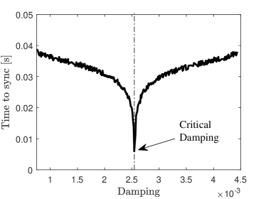
Figure 6: In a simulation of a network with $10$ generators, we measure the time it takes for each IBR to come within $.1$ Hz of the frequency of the large SG, after starting some fixed distance away. The parameter that is being varied is the value of the damping of generator $10$. Note that the critical damping $D_{n}=A_{n}/\omega_{R}$ very nearly minimizes the time to synchronization.

6 Closing Remarks and Outlook

Synchronization in electric power systems is one of the most intriguing open inquires that continues to attract scientists and engineers from various fields, given the structural characteristics that this class of complex system presents in the real-world: large-scale with a high degree of complexity. It presents a significant impact considering the serious ramifications that loss of synchronized operation in bulk power network will have; re-synchronizing a power grid is a daunting engineering task and prohibitively costly.

Here we focused on synchronization in heterogeneous power networks of many small generators and a single large generator, modeling grids with a large number of inverter-based resources with one large synchronous generator. While this model presents interesting results about the stability of synchronization, there are a number of areas in which this work could be expanded. This work relies on reduced networks through the use of Kron reduction, which produces a lower dimensional electrically equivalent network by aggregating the algebraic nodes and leveraging a sequential Gaussian elimination [46]. In future work, it would be of high interest to examine synchronization with the full, un-reduced network representation, which could provide insights that could be more readily applied to real world engineering practice. The hub and stoke topology adopted in this work is a special case that is possible in future decarbonized power grids that are expected to be more distributed with the capability to operate in both interconnected and islanded modes (including intentional islanding) to enhance the network resilience [45]. Thus, it would be interesting to examine multiple connected hub and spoke systems together, as these more closely resemble potential near-term power system topologies, including the phase transition as the network may reconfigure from an interconnected topology to an isolated island. In a similar vein, we have neglected the connections between the smaller generators that might exist in real-world systems, forming a meshed network. Though the synchronization linkages between small generators are likely to be weak, interesting cases may arise.

Synchronization in power networks is simply a steady evolution of frequency at each node, which inherently guarantees a steady flow of active power in the lines. However, recent literature has uncovered the importance of considering coupled voltage and frequency in power systems dominated by inverter-based resources [42, 34], because the assumption of constant voltage at generators used to derive the swing equation only applies to synchronous generators. Therefore, it would be illuminating to extend the current model from the classical swing equation to the two-dimensional planar swing equation, and examined frequency and voltage stability simultaneously [34, 42].

We believe our paper has a broader impact beyond power networks and the methods developed here could also be applied to other networks that follow a hub and spoke model for the identification of stability boundaries [44], analyses of structural properties [21], and understanding of bifurcation processes [2]. Such systems arise across a wide range of disciplines, including electrical engineering, mechanical engineering, network flows, vibration and acoustics, materials science, fluid dynamics and the biological sciences. We specifically identify strong parallels with a number of problems involving mechanical networks [47] and fluid suspensions with large mass ratios [41] , as well as mixtures of flows with large viscosity contrast [29], transportation networks [1], and logistics networks [33].

Appendix

Tables 1 and 2 below show the parameters used in the numerical simulations to generate the figures in the body of the text. In both cases, parameters were randomly assigned within physically meaningful ranges in such a way that oscillator $1$ has the largest mass and driving force, and so that oscillators with larger driving forces $A_{i}$ have larger coupling with oscillator $1$. This models the fact that larger generators tend to have more supply lines coupling them to the grid.

In Table 2, the primary value being varied is the damping of generator $n$, in order to create an under, critical, and over damping scenario. The other damping constants are adjusted slightly in such a way as to maintain a constant ratio $\left(\sum A\right)/\left(\sum D\right)$.

Table 1: Parameter values of the $15$ mass system network used to generate Figure 3.

Table 2: Parameter values of the $10$ generator network used to generate Figure 5.

References

- [1] Eric Agol, David M Hernandez, and Zachary Langford. A differentiable n-body code for transit timing and dynamical modelling–i. algorithm and derivatives. Monthly Notices of the Royal Astronomical Society, 507(2):1582–1605, 2021.
- [2] Fernando Alvarado, Ian Dobson, and Yi Hu. Computation of closest bifurcations in power systems. IEEE Transactions on Power Systems, 9(2):918–928, 1994.
- [3] T Athay, Robin Podmore, and Sudhir Virmani. A practical method for the direct analysis of transient stability. IEEE Transactions on Power Apparatus and Systems, (2):573–584, 1979.
- [4] PD Aylett. The energy-integral criterion of transient stability limits of power systems. Proceedings of the IEE-Part C: Monographs, 105(8):527–536, 1958.
- [5] Carl M. Bender and Steven A. Orszag. Advanced Mathematical Methods for Scientists and Engineers I: Asymptotic Methods and Perturbation Theory. Springer Science & Business Media, October 1999.
- [6] Sophie Boehm and Clea Schumer. 10 big findings from the 2023 ipcc report on climate change. 2023.
- [7] Hsiao-Dong Chiang, Chih-Wen Liu, Pravin P Varaiya, Felix F Wu, and Mark G Lauby. Chaos in a simple power system. IEEE Transactions on Power Systems, 8(4):1407–1417, 1993.
- [8] Michael T Craig, Ignacio Losada Carreño, Michael Rossol, Bri-Mathias Hodge, and Carlo Brancucci. Effects on power system operations of potential changes in wind and solar generation potential under climate change. Environmental Research Letters, 14(3):034014, 2019.
- [9] Michael T Craig, Stuart Cohen, Jordan Macknick, Caroline Draxl, Omar J Guerra, Manajit Sengupta, Sue Ellen Haupt, Bri-Mathias Hodge, and Carlo Brancucci. A review of the potential impacts of climate change on bulk power system planning and operations in the united states. Renewable and Sustainable Energy Reviews, 98:255–267, 2018.
- [10] Jeffrey Csank. Nasa lunar surface operations & power grid. In 11th Annual Center for Ultra-Wide-Area Resilient Electric Energy Transmission Networks (CURENT) Industry Conference, 2023.
- [11] Jeffrey Csank, George L. Thomas, Matthew Granger, and Brent Gardner. Powering the moon: From artemis technology demonstrations to a lunar economy. Nuclear and Emerging Technologies for Space (NETS-2022), 2022.
- [12] Biswa Nath Datta. Numerical linear algebra and applications (2. ed.). 2010.
- [13] Steven J Davis, Nathan S Lewis, Matthew Shaner, Sonia Aggarwal, Doug Arent, Inês L Azevedo, Sally M Benson, Thomas Bradley, Jack Brouwer, Yet-Ming Chiang, et al. Net-zero emissions energy systems. Science, 360(6396):eaas9793, 2018.
- [14] Florian Dörfler and Francesco Bullo. Synchronization and transient stability in power networks and nonuniform kuramoto oscillators. SIAM Journal on Control and Optimization, 50(3):1616–1642, 2012.
- [15] Florian Dörfler, Michael Chertkov, and Francesco Bullo. Synchronization in complex oscillator networks and smart grids. Proceedings of the National Academy of Sciences, 110(6):2005–2010, jan 2013.
- [16] Stephen George. Overview of Distributed Energy Resource Integration in ISO New England.
- [17] Dominic Groß and Florian Dörfler. On the steady-state behavior of low-inertia power systems. IFAC-PapersOnLine, 50(1):10735–10741, 2017.
- [18] John M. Guckenheimer and Philip Holmes. Nonlinear oscillations, dynamical systems, and bifurcations of vector fields. In Applied Mathematical Sciences, 1983.
- [19] Yufeng Guo, Dongrui Zhang, Zhuchun Li, Qi Wang, and Daren Yu. Overviews on the applications of the Kuramoto model in modern power system analysis. International Journal of Electrical Power & Energy Systems, 129:106804, July 2021.
- [20] Philip Hartman. A lemma in the theory of structural stability of differential equations. Proceedings of the American Mathematical Society, 11(4):610–620, 1960.
- [21] Marija Ilic, X Liu, B Eidson, C Vialas, and Michael Athans. A structure-based modeling and control of electric power systems. Automatica, 33(4):515–531, 1997.
- [22] Jesse D Jenkins and Samuel Thernstrom. Deep decarbonization of the electric power sector: Insights from recent literature. Energy Innovation Reform Project, 2017.
- [23] Jon Jensen and Nick Hatton. Impact of High Distributed Energy Resources.
- [24] Rick Wallace Kenyon, Matthew Bossart, Marija Markovic, Kate Doubleday, Reiko Matsuda-Dunn, Stefania Mitova, Simon A. Julien, Elaine T. Hale, and Bri-Mathias Hodge. Stability and control of power systems with high penetrations of inverter-based resources: An accessible review of current knowledge and open questions. Solar Energy, 210:149–168, 2020. Special Issue on Grid Integration.
- [25] Rick Wallace Kenyon, Amirhossein Sajadi, Matt Bossart, Andy Hoke, and Bri-Mathias Hodge. Interactive power to frequency dynamics between grid-forming inverters and synchronous generators in power electronics-dominated power systems, 2022.
- [26] Wlodzimierz Klonowski. Simplifying principles for chemical and enzyme reaction kinetics. Biophysical Chemistry, 18(2):73–87, 1983.
- [27] N. Kopell and R. Washburn. Chaotic motions in the two-degree-of-freedom swing equations. IEEE Transactions on Circuits and Systems, 29(11):738–746, 1982.
- [28] Benjamin Kroposki, Brian Johnson, Yingchen Zhang, Vahan Gevorgian, Paul Denholm, Bri-Mathias Hodge, and Bryan Hannegan. Achieving a 100% renewable grid: Operating electric power systems with extremely high levels of variable renewable energy. IEEE Power and energy magazine, 15(2):61–73, 2017.
- [29] Michael E Kurdzinski, Berrak Gol, Aaron Co Hee, Peter Thurgood, Jiu Yang Zhu, Phred Petersen, Arnan Mitchell, and Khashayar Khoshmanesh. Dynamics of high viscosity contrast confluent microfluidic flows. Scientific Reports, 7(1):5945, 2017.
- [30] Lazard Consultant. 2023 Levelized Cost Of Energy+, 2023.
- [31] K Loparo and G Blankenship. A probabilistic mechanism for dynamic instabilities in electric power systems. In Proc. IEEE Winter Power Meeting, New York, 1979.
- [32] Ignacio Losada Carreño, Michael T Craig, Michael Rossol, Moetasim Ashfaq, Fulden Batibeniz, Sue Ellen Haupt, Caroline Draxl, Bri-Mathias Hodge, and Carlo Brancucci. Potential impacts of climate change on wind and solar electricity generation in texas. Climatic Change, 163(2):745–766, 2020.
- [33] Cristina Masoller and Fatihcan M Atay. Complex transitions to synchronization in delay-coupled networks of logistic maps. The European Physical Journal D, 62:119–126, 2011.
- [34] Federico Milano. Complex frequency. IEEE Transactions on Power Systems, 37(2):1230–1240, 2021.
- [35] Federico Milano, Florian Dörfler, Gabriela Hug, David J Hill, and Gregor Verbič. Foundations and challenges of low-inertia systems. In 2018 Power Systems Computation Conference (PSCC), pages 1–25. IEEE, 2018.
- [36] Adilson E. Motter, Seth A. Myers, Marian Anghel, and Takashi Nishikawa. Spontaneous synchrony in power-grid networks. Nature Physics, 9(3):191–197, feb 2013.
- [37] Takashi Nishikawa and Adilson E Motter. Comparative analysis of existing models for power-grid synchronization. New Journal of Physics, 17(1):015012, jan 2015.
- [38] Louis Pecora and T. Carroll. Master stability functions for synchronized coupled systems. Phys. Rev. Lett., 80:2109–2112, 03 1998.
- [39] Faustino L Quintanilla. Palo Verde to Westwing Line 2 and Palo Verde to Rudd Double Line Outage Probability Analysis SRP.
- [40] Christopher Rackauckas and Qing Nie. DifferentialEquations.jl–a performant and feature-rich ecosystem for solving differential equations in Julia. Journal of Open Research Software, 5(1), 2017.
- [41] CQ Ru. Stokes’ second flow problem revisited for particle–fluid suspensions. Journal of Applied Mechanics, 91(4), 2024.
- [42] Amirhossein Sajadi and Bri-Mathias Hodge. Plane wave dynamic model of electric power networks with high shares of inverter-based resources. arXiv preprint arXiv:2401.16703, 2024.
- [43] Amirhossein Sajadi, Kenneth A Loparo, Robert D’Aquila, Kara Clark, Joseph G Waligorski, and Scott Baker. Great lakes o shore wind project: Utility and regional integration study. Technical report, Case Western Reserve Univ., Cleveland, OH (United States), 2016.
- [44] Amirhossein Sajadi, Robin Preece, and Jovica Milanović. Identification of transient stability boundaries for power systems with multidimensional uncertainties using index-specific parametric space. International Journal of Electrical Power & Energy Systems, 123:106152, 2020.
- [45] Amirhossein Sajadi, Luka Strezoski, Amin Khodaei, Kenneth Loparo, Mahmoud Fotuhi-Firuzabad, Robin Preece, Meng Yue, Fei Ding, Victor Levi, Pablo Arboleya, et al. Guest editorial: Special issue on recent advancements in electric power system planning with high-penetration of renewable energy resources and dynamic loads. International Journal of Electrical Power & Energy Systems, 129:106597, 2021.
- [46] Amirhossein Sajadi, Rick Wallace, and Bri-Mathias Hodge. Synchronization in electric power networks with inherent heterogeneity up to 100% inverter-based renewable generation. Nature Communications, 13(1), may 2022.
- [47] Malcolm C Smith. Synthesis of mechanical networks: the inerter. IEEE Transactions on automatic control, 47(10):1648–1662, 2002.
- [48] Doug Tucker, Dmitry Kosterev, and Amirhossein Sajadi. Frequency response in the western interconnection with significantly high shares of inverter-based resources: 100 In 2022 IEEE Power & Energy Society General Meeting (PESGM), pages 1–5, 2022.
- [49] Andreas Ulbig, Theodor S Borsche, and Göran Andersson. Impact of low rotational inertia on power system stability and operation. IFAC Proceedings Volumes, 47(3):7290–7297, 2014.
- [50] Richard S. Varga. Gersgorin and his circles. 2004.
- [51] Yuanzhao Zhang, Jorge L. Ocampo-Espindola, István Z. Kiss, and Adilson E. Motter. Random heterogeneity outperforms design in network synchronization. Proceedings of the National Academy of Sciences, 118(21), May 2021.