Matching 2D Images in 3D: Metric Relative Pose from Metric Correspondences

Abstract

Given two images, we can estimate the relative camera pose between them by establishing image-to-image correspondences. Usually, correspondences are 2D-to-2D and the pose we estimate is defined only up to scale. Some applications, aiming at instant augmented reality anywhere, require scale-metric pose estimates , and hence, they rely on external depth estimators to recover the scale. We present MicKey, a keypoint matching pipeline that is able to predict metric correspondences in 3D camera space. By learning to match 3D coordinates across images, we are able to infer the metric relative pose without depth measurements. Depth measurements are also not required for training, nor are scene reconstructions or image overlap information. MicKey is supervised only by pairs of images and their relative poses. MicKey achieves state-of-the-art performance on the Map-Free Relocalisation benchmark while requiring less supervision than competing approaches.

1 Introduction

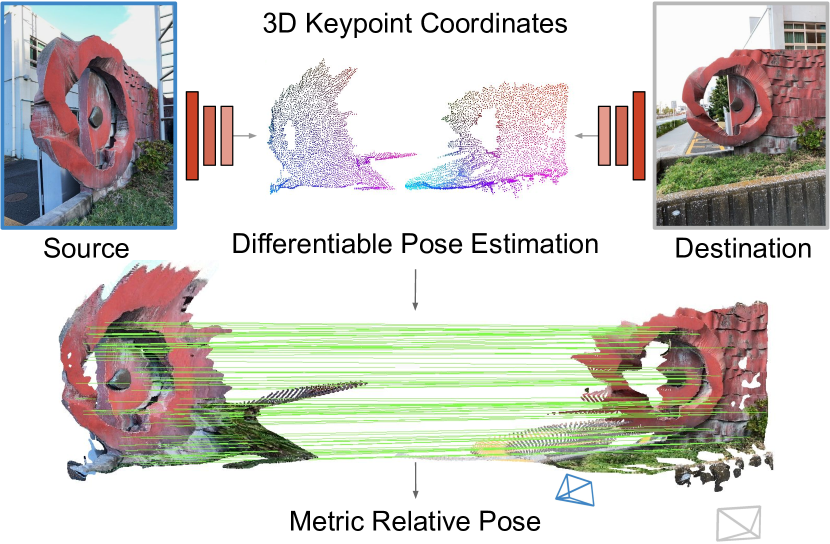
Figure 1: We introduce MicKey, a neural network that predicts 3D metric keypoint coordinates in camera space from a 2D input image. Given two images, MicKey establishes 3D-3D correspondences via descriptor matching and then applies a Kabsch [41] solver to recover the metric relative pose. We visualize the 3D keypoint coordinates by mapping them to the RGB cube.

Whether you prefer inches or centimeters, we measure and understand the world in scale-metric units. Unfortunately, the scale-metric quality of the world is lost when we project it to the image plane. The scale-ambiguity is one aspect that makes computer vision, and building applications on top of it, hard. Imagine an augmented reality problem where two people look at the same scene through their phones. Assume we want to insert scaled virtual content, e.g., a virtual human, into both views. To do that in a believable fashion, we need to recover the relative pose between both cameras and we need it up to scale [75, 2].

Estimating the relative pose between two images is a long-standing problem in computer vision [29, 57, 56]. Solutions based on feature matching offer outstanding quality even under adverse conditions like wide baseline matching or changing seasons [40]. However, their geometric reasoning is limited to the 2D plane, so the distance between the cameras remains unknown [36, 2].

In some settings, we can resort to dedicated hardware to recover the scene scale. Modern phones come with IMU sensors, but they require the user to move [63]. Some phones come with LiDAR sensors that measure depth, but these sensors are limited in terms of range and constrained to very few high-end devices [32].

The general setting, as recently formalized as “Map-free Relocalisation” [2], provides only two images and intrinsics but no further measurements. The best solution to recover a metric relative pose hitherto was to combine 2D feature matching with a separate depth estimation network to lift correspondences to 3D metric space. However, there are two problems. Firstly, the feature detector and the depth estimator are separate components that operate independently. Feature detectors generally fire on corners and depth discontinuities [5, 22, 58], exactly the areas where depth estimators struggle. Secondly, learning the best metric depth estimators usually requires strong supervision with ground truth depth which can be hard to come by, depending on the data domain [65]. E.g., for pedestrian imagery recorded by phones, measured depth is rarely available.

We present Metric Keypoints (MicKey), a feature detection pipeline that addresses both problems. Firstly, MicKey regresses keypoint positions in camera space which allows us to establish metric correspondences via descriptor matching. From metric correspondences, we can recover the metric relative pose, see Figure 1. Secondly, by training MicKey in an end-to-end fashion using differentiable pose optimization, we require only image pairs and their ground truth relative poses for supervision. Depth measurements are not required. MicKey learns the correct depth of keypoints implicitly, and only for areas where features are actually found and are accurate. Our training procedure is robust to image pairs with unknown visual overlap, and therefore, information such as image overlap, usually acquired via structure-from-motion reconstructions [51], is not needed. This weak supervision makes MicKey very accessible and attractive, since training it on new domains does not require any additional information beyond the poses.

MicKey ranks among the top-performing methods in the Map-free Relocalization benchmark [2], surpassing very recent, state-of-the-art approaches. MicKey provides reliable, scale-metric pose estimates even under extreme viewpoint changes enabled by depth predictions that are specifically tailored towards sparse feature matching.

We summarize our contributions as follows: 1) A neural network, MicKey, that predicts metric 3D keypoints and their descriptors from a single image, allowing metric relative pose estimation between pairs of images. 2) An end-to-end training strategy, that only requires relative pose supervision, and thus, neither depth measurements nor knowledge about image pair overlap are needed during training.

2 Related Work

Relative Pose by Keypoint Matching. In the calibrated scenario, where camera intrinsics are known, the relative camera pose can be recovered by decomposing the essential matrix [36]. The essential matrix is normally computed by finding keypoint correspondences between images, and then applying a solver, e.g., the 5-point algorithm [62], within a RANSAC [30] loop. Classical keypoint correspondences were built around SIFT [54], however, latest learned methods have largely superseded it. Keypoint detectors [83, 5, 48], path-based descriptors [76, 77], joint keypoint extractors [22, 6, 66, 24, 55, 33], or affine shape estimators [88, 59, 7] are now able to compute more accurate and distinctive features. Learned matchers [69, 52], detector-free algorithms [73, 39, 80, 25, 17], outlier rejection methods [89, 92, 91, 74, 16], or better robust estimators [78, 20, 79, 12, 8] can improve further the quality of the estimated essential matrices. However, the essential matrix decomposition results in a relative rotation matrix and a scaleless translation vector. It does not yield the distance between the cameras. Arnold et al. [2] show that matching methods can resolve the scale ambiguity via metric depth estimators [28, 72]. Single-image depth prediction can regress the absolute depth in meters [65, 53, 84], being able then to lift 2D points to 3D metric coordinates, where PnP [31] or Kabsch (also called orthogonal Procrustes) [41, 27] can recover the metric relative pose from the 2D-3D or the 3D-3D correspondences, respectively.

Relative Pose Regression (RPR) methods propose an alternative strategy to recover relative poses. They encode the two images within the same neural network and directly estimate their relative pose as their output. Contrary to scene coordinate regression [71, 50, 11] or absolute pose regression [44, 43, 70], RPR [4, 15, 87, 45, 18] does not require being trained on specific scenes, making them very versatile. Arnold et al. [2] propose different variants of RPR networks to tackle their AR anywhere task. Since they do not require depth maps, Arnold et al. train their RPR networks with the supervision provided in the Map-free dataset: poses and overlap scores. The biggest limitation of RPR methods is that they do not provide any confidence for their estimates, making them unreliable in practice [2].

Differentiable RANSAC enables optimizing pipelines that predict model parameters, e.g., camera pose parameters, directly via end-to-end training [14, 12, 85]. NG-DSAC [12], a combination of DSAC [14] and NG-RANSAC [12], provides gradients of RANSAC-fitted camera poses w.r.t. the coordinates and confidences of input correspondences. NG-DSAC uses score function-based gradient estimates, i.e., policy gradient [23] and REINFORCE [86]. Besides learning visual relocalization [14, 12], policy gradient has also been used for learning keypoint detectors and descriptors [61, 68, 10, 49]. $\nabla$-RANSAC [85] is a differentiable RANSAC variation based on path derivative gradient estimators using the Gumbel softmax trick [38].

Contrary to previous keypoint extractors, MicKey requires learning the 3D coordinates of keypoints. We combine NG-DSAC with the Kabsch [41] algorithm, a differentiable solver, and learn directly from pose signals. To the best of our knowledge, although learning from poses has been explored [67, 85], we are the first to propose a strategy that optimizes directly 3D keypoint coordinates towards metric relative pose estimation.

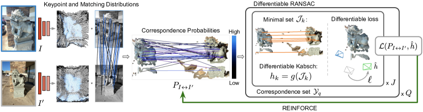
Figure 2: Training pipeline. MicKey predicts 3D coordinates of keypoints in camera space. The network also predicts keypoint selection probabilities (keypoint distribution) and descriptors that steer the probabilities of matches (matching distribution). The combination of both distributions yields the probability of two keypoint being a correspondence in $P_{I\leftrightarrow I^{\prime}}$, and we optimize the network such that correct correspondences are more likely. Within a differentiable RANSAC loop, we generate multiple relative pose hypotheses and compute their loss w.r.t. to the ground truth transformation, $\hat{h}$. We generate gradients to train the correspondence probabilities $P_{I\leftrightarrow I^{\prime}}$ via REINFORCE. Since our pose solver and loss function are differentiable, backpropagation also provides a direct signal to train the 3D keypoint coordinates.

3 Method

This section first introduces the main blocks of our differentiable pose solver and then defines our new architecture.

3.1 Learning from Metric Pose Supervision

Given two images, our system computes their metric relative pose along with the keypoint scores, the match probabilities, and the pose confidence (in the form of soft-inlier counting). We aim to train all our relative pose estimation blocks in an end-to-end fashion. During training, we assume to have training data as ($I$, $I^{\prime}$, $T^{GT}$, $K$, $K^{\prime}$), with $T^{GT}$ being the ground truth transformation and $K/K^{\prime}$ the camera intrinsics. The full system is pictured in Figure 2.

To learn 3D keypoint coordinates, confidences, and descriptors, we require our system to be fully differentiable, and since some of the elements of the pipeline are not, e.g., keypoint sampling or inlier counting, we redefine the relative pose estimation pipeline as probabilistic. That means that we treat the output of our network as probabilities over potential matches, and during training, the network optimizes its outputs to generate probabilities that make correct matches more likely to be selected.

3.1.1 Probabilistic Correspondence Selection

A keypoint is characterized by a 3D coordinate, a descriptor, and a confidence value. We obtain the descriptor and the confidence directly from the output of the network, meanwhile, the 3D coordinate, $x$, is defined via a 2D position, $\bar{u}$, and a depth value, $z$:

$$\begin{gathered}x=z\cdot K^{-1}\bar{u}^{T}.\vspace{-1.0em}\end{gathered}$$ (1)

For notation simplicity, we assume homogeneous coordinates for the 2D point $\bar{u}$. A correspondence $y$ is defined by a keypoint in $I$ and a keypoint in $I^{\prime}$, and we refer to a set of keypoint correspondences as $\mathcal{Y}$. We formulate the probability of drawing $\mathcal{Y}$ as the product of the probabilities of sampling them individually ($P(\mathcal{Y})=\Pi\,P(y_{ij})$). Specifically, we define a correspondence $y_{ij}$ as a tuple of 3D point coordinates, $y_{ij}=(x_{i},x^{\prime}_{j})$, where $x_{i}$ refers to keypoint $i$ from $I$, and $x^{\prime}_{j}$ to the keypoint $j$ from $I^{\prime}$. We will define the probability of sampling that correspondence next.

Correspondence Probability. The total probability of sampling a keypoint correspondence $P(y_{ij})$ is modelled as a function of their descriptor matching and keypoint selection probabilities, such that:

$$\begin{gathered}P(y_{ij})=\underbrace{P_{I}(i)\cdot P_{I\rightarrow I^{\prime}}(j|i)}_{\text{forward matching}}\cdot\underbrace{P_{I^{\prime}}(j)\cdot P_{I\leftarrow I^{\prime}}(i|j)}_{\text{backward matching}}.\end{gathered}$$ (2)

Forward matching combines the probability of selecting keypoint $i$ in image $I$, denoted $P_{I}(i)$, and the probability of $j$ in image $I^{\prime}$ being the nearest neighbor of $i$, denoted $P_{I\rightarrow I^{\prime}}(j|i)$. The backward matching probability is defined accordingly. We define the matrix containing all possible correspondence probabilities as $P_{I\leftrightarrow I^{\prime}}$, where $P_{I\leftrightarrow I^{\prime}}(i,j)=P(y_{ij})$. We formulate the descriptor matching and keypoint selection probabilities as follows:

Matching Distribution. The descriptor matching probability represents the probability of two keypoints being mutual nearest neighbors, i.e., keypoint $i$ matches $j$, and keypoint $j$ matches $i$. For that, we first compute the probability of $j$ being the nearest neighbor to $i$ conditioned on $i$ already being selected as a keypoint: $P_{I\rightarrow I^{\prime}}(j|i)$. We obtain that probability by applying a Softmax over all the similarities of $j$ for a fixed $i$:

$$\begin{gathered}P_{I\rightarrow I^{\prime}}(j|i)=\text{Softmax}(m(i,\cdot)/\theta_{m})_{j},\end{gathered}$$ (3)

where $m$ is the matrix defining all descriptor similarities and $\theta_{m}$ is the descriptor Softmax temperature. Before the Softmax operator, we augment $m$ with a single learnable dustbin parameter to allow unmatched keypoints to be assigned to it [69]. We remove the dustbin after the Softmax operator. Equivalently, we obtain $P_{I\leftarrow I^{\prime}}(i|j)$. Therefore, the mutual nearest neighbor consistency, $P_{I\rightarrow I^{\prime}}(j|i)\cdot P_{I\leftarrow I^{\prime}}(i|j)$, is enforced by the dual-Softmax operator as in [81, 73, 26].

Keypoint Distribution. The keypoint selection probability represents the probability of two independent keypoints being sampled. I.e., probability $P_{I}(i)$ of $i$ being selected from image $I$, and the probability $P_{I^{\prime}}(j)$ of $j$ being selected from $I^{\prime}$. We compute $P_{I}(i)$ by applying a spatial Softmax over all confidence values predicted by the network from image $I$, and, similarly, $P_{I^{\prime}}(j)$ is obtained from the Softmax operator over all confidences from $I^{\prime}$.

3.1.2 Differentiable RANSAC

Due to the probabilistic nature of our approach and potential errors in our network predictions, we rely on the robust estimator RANSAC [30] to compute pose hypotheses $h$ from $\mathcal{Y}$. We require our RANSAC layer to backpropagate the pose error to the keypoints and descriptors, and hence, we follow differentiable RANSAC works [10, 13, 12], and adjust them as necessary for our problem:

Generate hypotheses. Given the correspondences $\mathcal{Y}$, we use the probability values defined in $P_{I\leftrightarrow I^{\prime}}$ to guide the new sampling of $J$ subsets: $\mathcal{J}_{k}\subset\mathcal{Y}$, with $0\leq k<J-1$. Every subset is defined by n 3D-3D correspondences in camera coordinates and generates a pose hypothesis $h_{k}$ that is recovered by a differentiable pose solver $g$, i.e., $h_{k}=g(\mathcal{J}_{k})$.

Differentiable Kabsch. We use the Kabsch pose solver [41] for estimating the metric relative pose from the subset of correspondences $\mathcal{J}_{k}$. The Kabsch solver finds the pose that minimizes the square residual over the 3D-3D input correspondences:

$$\begin{gathered}g^{\text{Kabsch}}(\mathcal{J})=\operatorname*{argmin}_{h}\sum_{y\in\mathcal{J}}r(y,h)^{2}.\end{gathered}$$ (4)

The residual error function $r(\cdot)$ computes the Euclidean distance between 3D keypoint correspondences after applying the pose transformation $h$. All the steps within the Kabsch solver are differentiable and have been previously studied. We refer to [13, 3] for additional details.

Soft-Inlier Counting. Since counting inliers is not differentiable, we compute a differentiable approximation of the inlier counting (soft-inlier counting) by replacing the hard threshold with a Sigmoid function $\sigma(\cdot)$. The soft-inlier counting is done over the complete set of correspondences $\mathcal{Y}$:

$$\begin{gathered}s(h,\mathcal{Y})=\sum_{y\in\mathcal{Y}}\sigma[\beta\tau-\beta r(y,h)].\end{gathered}$$ (5)

$\beta$ controls the softness of the Sigmoid. As in [13], we set $\beta$ in dependence of the inlier threshold $\tau$ such that $\beta=\frac{5}{\tau}$.

Differentiable Refinement. We refine the pose hypothesis $h$ by iteratively finding its correspondence inliers $\mathcal{I}$ and recomputing a new pose from them:

$$\begin{gathered}h^{t+1}=g(\mathcal{I}^{t})\quad\text{and}\quad\mathcal{I}^{t+1}=\{i|r(y_{i},h^{t+1})<\tau\}.\end{gathered}$$ (6)

We repeat the process until a maximum number of iterations $t_{\text{max}}$ is reached, or the number of inliers stops growing. We refer to the refinement step as $R(h,\mathcal{Y})$, and approximate its gradients by fixing and backpropagating only through its last iteration [13].

3.1.3 Learning Objective

We use the Virtual Correspondence Reprojection Error (VCRE) metric proposed in [2] as our loss function. VCRE defines a set of virtual 3D points ($\mathcal{V}$) and computes the Euclidean error of its projections in the image:

$$\begin{gathered}\ell^{\text{VCRE}}(h,\hat{h})=\frac{1}{|\mathcal{V}|}\sum_{v\in\mathcal{V}}||\pi(v)-\pi(h\hat{h}^{-1}v)||_{2},\end{gathered}$$ (7)

with $\hat{h}=T^{GT}$ and $\pi$ being the projection function. Refer to Section B for more details on VCRE. For each $\mathcal{Y}$, we compute a set of hypotheses $h_{k}$ with corresponding scores $s_{k}$, and define its loss following DSAC [14]:

$$\begin{gathered}\ell({\mathcal{Y}},\hat{h})=\operatorname{\mathbb{E}}_{k\sim p(k|\mathcal{Y})}[\ell^{\text{VCRE}}(R(h_{k},\mathcal{Y}),\hat{h})].\end{gathered}$$ (8)

We derive the probability of each hypothesis, $p(k|\mathcal{Y})$, from its score $s_{k}$ via Softmax normalization. Since the expectation above is defined over a finite set of hypotheses, we can solve it exactly to yield a single loss value for $\mathcal{Y}$.

Our final optimization is formulated as a second, outer expectation of the VCRE loss by sampling correspondence sets $\mathcal{Y}_{q}$ from the correspondence matrix $P_{I\leftrightarrow I^{\prime}}$:

$$\begin{gathered}\mathcal{L}(P_{I\leftrightarrow I^{\prime}},\hat{h})=\operatorname{\mathbb{E}}_{q\sim p(q|P_{I\leftrightarrow I^{\prime}})}[\ell({\mathcal{Y}_{q}},\hat{h})].\end{gathered}$$ (9)

From now on, we abbreviate $\mathcal{L}(P_{I\leftrightarrow I^{\prime}},\hat{h})$ to $\mathcal{L}$ and $\ell({\mathcal{Y}_{q}},\hat{h})$ to $\ell$. We can approximate the gradients of $\mathcal{L}$ w.r.t. to network parameters ($w$) by drawing $Q$ samples:

$$\begin{gathered}\frac{\partial}{\partial w}\mathcal{L}\approx\frac{1}{Q}\sum_{q\in Q}[\ell\frac{\partial}{\partial w}\text{log}P_{I\leftrightarrow I^{\prime}}+\frac{\partial}{\partial w}\ell],\end{gathered}$$ (10)

where the first term provides gradients to learn descriptors and keypoint confidences, steering the sampling probability $P_{I\leftrightarrow I^{\prime}}$ in a good direction. The second term provides directly the gradients to optimize the 2D keypoint offsets and the depth estimations. To reduce the variance of Equation 10, we follow [12] by subtracting a baseline $b=\bar{\ell}$ from $\ell$, the mean loss over all samples:

$$\begin{gathered}\frac{\partial}{\partial w}\mathcal{L}\approx\frac{1}{Q}\sum_{q\in Q}[[\ell-b]\frac{\partial}{\partial w}\text{log}P_{I\leftrightarrow I^{\prime}}+\frac{\partial}{\partial w}\ell].\end{gathered}$$ (11)

3.1.4 Curriculum Learning

Initialization is an important and challenging step when learning only from poses, since networks might not be able to converge without it [10]. One common solution in reinforcement learning is to feed the network with increasingly harder examples that may otherwise be too difficult to learn from scratch [60]. However, contrary to other methods [69, 73, 25], we aim at training our network without requiring to know what easy or hard examples are. Instead of using all image pairs in a training batch $B$, we optimize the network only using a subset of image pairs. We select the image pairs that return the lowest losses and ignore all others, i.e., the network is optimized only with the examples that it can solve better, and hence, are easier. As we progress in the training, we increase the fraction of examples from $B$ that the network needs to solve. We define both, the minimum and maximum number of pairs ($b_{\text{min}}$ and $b_{\text{max}}$), used in training.

Even though we limit the optimization to the best pose estimates, the network might still try to optimize an image pair where all RANSAC hypotheses are incorrect. Since hypotheses scores are normalized per image pair, see Equation 8, incorrect hypotheses can add noise to the optimization. To mitigate this, we add a null hypothesis ($h^{0}$) to Equation 8. The null hypothesis has a fixed score $s^{0}$ as well as a fixed loss $\ell^{\text{VCRE}}(h^{0},\hat{h})=\text{VCRE}^{\text{max}}$, where $\text{VCRE}^{\text{max}}$ is the maximum value we tolerate as a good pose. $h^{0}$ serves as an anchor point, such that the network can assign lower scores than $s^{0}$ to hypotheses with high error. If all hypotheses in a pool are incorrect with low scores, the null hypothesis will dominate the expectation in Equation 8 and reduce the impact of gradients from the remaining hypotheses.

3.2 Architecture

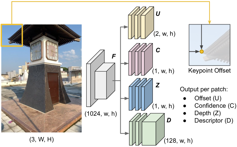
Figure 3: MicKey Architecture. MicKey uses a feature extractor that splits the image into patches. For every patch, MicKey computes a 2D offset, a keypoint confidence, a depth value, and a descriptor vector. The 3D keypoint coordinates are obtained by the absolute position of the patch, its 2D offset, and depth value.

MicKey follows a multi-head network architecture with a shared encoder [81, 66, 22] that infers 3D metric keypoints and descriptors from an input image as seen in Figure 3.

Encoder. We adopt a pre-trained DINOv2 as our feature extractor [64] and use its features without further training or fine-tuning. DINOv2 divides the input image into patches of size $14\times 14$ and provides a feature vector for each patch. The final feature map, $F$, has a resolution of $(1024,w,h)$, where $w=W/14$ and $h=H/14$.

Keypoint Heads. We define four parallel heads that process the feature map $F$ and compute the xy offset ($U$), depth ($Z$), confidence ($C$), and descriptor ($D$) maps; where each entry of the maps corresponds to a $14\times 14$ patch from the input image. Similar to [19], MicKey has the rare property of predicting keypoints as relative offsets to a sparse regular grid. We obtain the absolute 2D coordinates ($\bar{U}$) as:

$$\begin{gathered}\bar{u}_{ij}=f*[u_{i}+i,u_{j}+j],\text{with }u\in[0,1],\end{gathered}$$ (12)

where f refers to the encoder downsampling factor ($f=14$) and $ij$ to the grid position. Since MicKey predicts coordinate offsets over a coarse grid, it remains efficient while still providing correspondences with sub-pixel accuracy. Note that instead of applying a local non-maxima suppression [81, 55], MicKey already provides a single keypoint location for every input patch.

Map-free Dataset
				VCRE			Median Errors			Matching		Estimates
				AUC	Prec. (%)		Rep. (px)	Trans. (m) / Rot. (°)		Time (ms)		(%)
		SIFT [54]		0.50	25.0		222.8	2.93 / 61.4		157.6		100.0
		SiLK [33]		0.31	18.0		176.4	2.20 / 33.8		58.4		52.1
Depth + Overlap + Pose Supervision		Sparse Features
		DISK [81]		0.54	26.8		208.1	2.59 / 51.9		58.7		99.9
		DeDoDe [26]		0.53	31.2		167.4	2.02 / 30.2		200.3		88.0
		SuperPoint [22] - SuperGlue [69]		0.60	36.1		160.3	1.88 / 25.4		95.6		100.0
		DISK [81] - LightGlue [52]		0.53	33.2		138.8	1.44 / 18.5		108.5		77.9
		Dense Features
		LoFTR [73]		0.61	34.7		167.6	1.98 / 30.5		114.9		100.0
		ASpanFormer [17]		0.64	36.9		161.7	1.90 / 29.2		177.1		99.9
		RoMa [25]		0.67	45.6		128.8	1.23 / 11.1		820.2		99.9
No Depth Supervision		Overlap + Pose Supervision
		RPR [R($\alpha,\beta,\gamma$) + s$\cdot$t($\theta,\omega$)] [2]		0.35	35.4		166.3	1.83 / 23.2		21.6		100.0
		RPR [3D-3D] [2]		0.39	38.7		148.7	1.69 / 22.9		25.3		100.0
		RPR [R(6D) + t] [2]		0.40	40.2		147.1	1.68 / 22.5		24.3		100.0
		MicKey w/ Overlap (ours)		0.75	49.2		129.4	1.65 / 27.2		119.8		100.0
2-13		Pose Supervision
		RPR [R(6D) + t] w/o Overlap		0.18	18.1		197.1	2.45 / 34.7		24.3		100.0
		MicKey (ours)		0.74	49.2		126.9	1.59 / 25.9		119.8		100.0

Table 1: Relative pose evaluation on the Map-free dataset. We report the area under the curve (AUC) and precision (Prec.) values for the VCRE metric under a threshold of 90 pixels as in [2], where both versions of MicKey obtain the top results. Besides, we also report the median errors, and while MicKey obtains the lowest value in terms of VCRE error, other methods, e.g., RoMa, provide lower pose errors. To compute the median errors, the benchmark only uses the valid poses generated by each method, and hence, we report the total number of estimated poses. Lastly, we report the matching times and see that MicKey is at par with LoFTR and LighGlue, while reducing significantly the time of RoMa, its closest competitor in terms of VCRE metrics. Matching methods use DPT [65] to recover the scale.

4 Experiments

This section first presents details of our implementation and training pipeline, and then discusses the results for different methods in the task of instant AR at new locations.

Inference vs Training. We use the same probabilistic solver in training and testing, however, some of its parameters change. During training, given the set of correspondences $\mathcal{Y}$, we perform 20 RANSAC iterations ($J=20$), and in each one, we sample 5 correspondences ($n=5)$. Although Kabsch only requires a minimal set of 3 correspondences, we found more stable gradients when increasing it. In training, we refine all generated hypotheses. At test time, we increase the number of iterations to $J=100$ and use minimal sets of size $n=3$ in Kabsch. Moreover, we select the best hypothesis based on the soft-inlier score and only refine the winning one. The number of maximum refinement iterations $t_{\text{max}}=4$ and the number of $\mathcal{Y}$ samplings $Q=20$ is the same in training and testing. Refer to Section B for more details about the training pipeline.

Map-free Benchmark [2] evaluates the ability of methods to allow AR experiences at new locations. This task-oriented benchmark uses two images, the reference, and the query, and determines whether their estimated metric relative pose is acceptable or not for AR. A pose is accepted as good if their VCRE, see Section 3.1.3, is below a threshold. Specifically, the authors argue that an offset of 10% of the image diagonal would provide a good AR experience. In the Map-free dataset, this corresponds to 90 pixels. We follow the protocol from Map-free in two datasets; Map-free for outdoor, and ScanNet [21] for indoor scenes.

4.1 Map-free Dataset

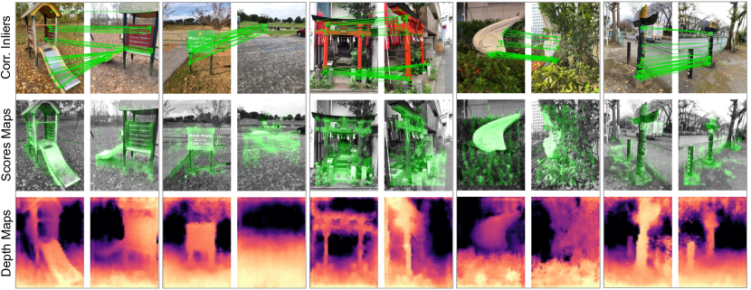
Figure 4: Example of correspondences, scores and depth maps generated by MicKey. MicKey finds valid correspondences even under large-scale changes or wide baselines. Note that the depth maps have a resolution 14 times smaller than the input images due to our feature encoder. We follow the visualization of depth maps used in DPT [65], where brighter means closer.

Map-free dataset contains 460, 65, and 130 scenes for training, validation, and test, respectively. Each training scene is composed of two different scans of the scene, where absolute poses are available. In the validation and test set, data is limited to a reference image and a sequence of query images. The test ground truth is not available, and hence, all results are evaluated through the Map-free website. We compare MicKey against different feature matching pipelines and relative pose regressors (RPR). All matching algorithms are paired with DPT [65] for recovering the metric scale. Besides, we present two versions of MicKey, one that relies on the overlap score and uses the whole batch during training, and another that follows our curriculum learning strategy (Section 3.1.4). For MicKey w/ Overlap, we use the same overlap range proposed in [2] (40%-80%). Evaluation in the Map-free test set is shown in Table 3.2.

The benchmark measures the capability of methods for an AR application, and instead of focusing on the relative pose errors, it quantifies the quality of such algorithms in terms of a reprojection error metric in the image plane (VCRE), claiming that this is more correlated with a user experience [2]. Specifically, the benchmark looks into the area under the curve (AUC) and precision value (Prec.). The AUC takes into account the confidence of the network, and hence, it also evaluates the capability of the methods to decide whether such estimations should be trusted. The precision measures the percentage of estimations under a threshold (90 pixels). We observe that the two variants of MicKey provide the top VCRE results, both in terms of AUC and precision. We see little benefit from training MicKey with also the overlap score supervision and claim that if such data is not available, our simple curriculum learning approach yields top performance. Besides, we note that training naively RPR methods without the overlap scores (RPR w/o Overlap) degrades considerably the performance.

The benchmark also provides the reprojection error of the virtual correspondences in the image plane (see Equation 7), and the standard translation (m) and rotation (°) errors of the poses w.r.t. the ground truth. Refer to Section C.2 for more metrics and details. The median errors are computed only using valid poses, and thus, we report the total percentage of estimated poses. MicKey gets the lowest reprojection error, while RoMa [25] obtains the lowest pose errors. Although RoMa estimates are very precise, we show in Section C.2 that its confidence values have low reliability, not providing a good mechanism to decide whether such poses should be trusted. DISK [81] - LightGlue [52] also provide accurate estimations, but they only provide 77.9% of the total poses, meaning that the median errors are computed only for a subset of the test set.

Lastly, for a new query image, we compute the time needed to obtain the keypoint correspondences and their 3D coordinates, i.e., xy positions and depths. In the case of RPR, since they do direct pose regression, we report their inference time. MicKey has comparable times w.r.t. other matching competitors, e.g., LoFTR or LightGlue, while reducing by 85% the time of RoMa, the second best method.

4.2 ScanNet Dataset

Contrary to the Map-free evaluation, where depth or matching methods were trained in a different outdoor domain, we evaluate results on ScanNet [21], which has ground truth depths, overlap scores, and poses available for training. We use the training, validation, and test splits proposed by SuperGlue [69] and used in following works [2, 73, 17]. To recover the scale of matching methods, we use PlaneRCNN [53], which was trained on ScanNet and yields higher quality metric poses (see Section C.1 for more details).

Evaluation in ScanNet test set is shown in Table 2. We use the same criteria as in the Map-free benchmark and evaluate the VCRE poses under the 10% of the image diagonal. Contrary to Map-free, ScanNet test pairs ensure that input images overlap, and results show that all methods perform well under these conditions. Similar to previous experiment, we observe that MicKey does not benefit much from using the overlap scores during training. Therefore, results show that training MicKey with only pose supervision obtains comparable results to fully supervised methods, proving that state-of-the-art metric relative pose estimators can be trained with as little supervision as relative poses.

ScanNet Dataset
	VCRE			Median Errors
	AUC	Prec. (%)		Trans (m) / Rot (°)
D+O+P Signal
SuperGlue [22, 69]	0.98	90.6		0.15 / 2.06
LoFTR [73]	0.99	91.3		0.13 / 1.81
ASpanFormer [17]	0.99	90.6		0.14 / 1.48
RoMa [25]	0.99	94.4		0.11 / 1.47
O+P Signal
RPR [R + s·t] [2]	0.85	85.0		0.25 / 4.12
RPR [3D-3D] [2]	0.93	92.8		0.20 / 4.05
MicKey-O (ours)	0.99	93.7		0.17 / 3.58
Pose Signal
RPR [3D-3D]	0.78	78.3		0.55 / 5.12
MicKey (ours)	0.99	92.8		0.17 / 3.64

Table 2: Relative pose evaluation on ScanNet dataset. All feature matching methods are coupled with PlaneRCNN [53] for recovering the metric scale. We indicate the training signal of each method as: depth (D), overlap score (O), and pose (P).

4.2.1 Understanding MicKey

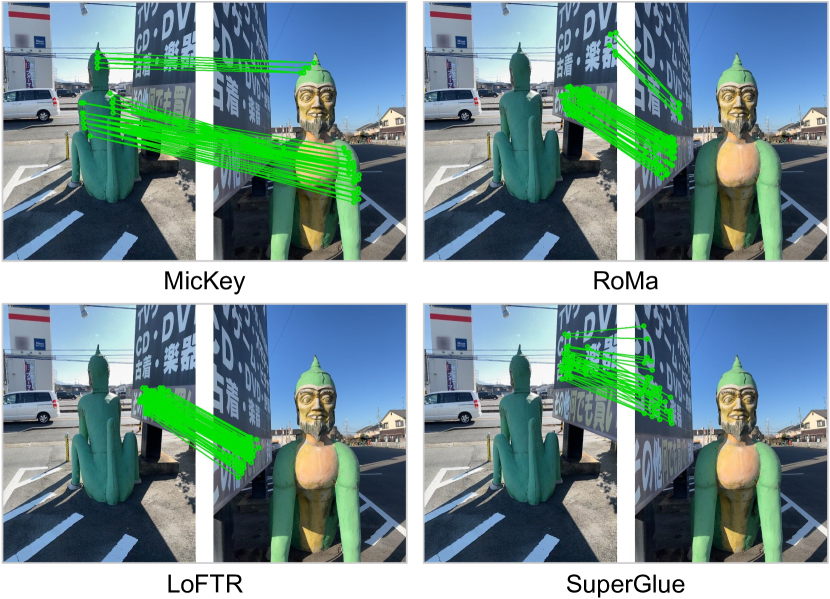
Figure 5: MicKey establishes keypoint correspondences even though images share very little visual overlap. Contrary to other matchers, MicKey does not focus on the textured wall, but instead reasons about the shape of the object in the foreground.

Map-free Dataset
	VCRE			Median Errors
	AUC	Prec. (%)		Trans (m) / Rot (°)
SuperGlue [22, 69]
DPT [65]	0.60	36.1		1.88 / 25.4
KBR [72]	0.61	35.7		1.92 / 25.4
Our Depth	0.71	43.0		1.69 / 25.4
LoFTR [73]
DPT [65]	0.61	34.7		1.98 / 30.5
KBR [72]	0.60	32.1		2.11 / 30.5
Our Depth	0.71	40.7		1.92 / 30.5

Table 3: Depth ablation. Due to MicKey’s end-to-end nature, MicKey’s depth maps have been designed to provide accurate depths where keypoints are detected, boosting the performance of state-of-the-art sparse and dense feature matchers.

Depth Evaluation in Table 3 shows that state-of-the-art matchers obtain top performance when paired with our depth maps. Even though other depth methods [65, 72] could be trained on Map-free data, it is unclear how standard photometric losses [34, 35, 90, 93] would work across scans, where images could have large baselines, and whether such methods would generate better depth maps for the metric pose estimation task. We visualize our depth maps in Figure 4, where we also display MicKey’s score maps and correspondence inliers. We see that the score maps highlight the areas of the image where the object of interest is, and it does not fire only on corners and edges. The detector and depth heads are tailored during training, and hence, the detector learns to use the positions where the depth is accurate.

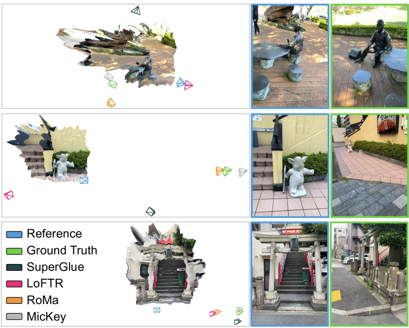
Figure 6: Visualization of relative camera poses. In this visualization, we use Map-free validation scenes and visualize the different predicted poses w.r.t. the ground truth (green camera).

Beyond Low-level Matching. Figure 5 displays an image pair where almost no visual overlap is shared between the images. In that example, we see that MicKey exhibits a different behavior than the other matchers, where instead of focusing on the low-level patterns of the wall, it reasons about the shape of the object, showing glimpses of high-level reasoning. State-of-the-art competitors have been trained with the premise that image pairs have a minimum overlap, meanwhile, our flexible training pipeline uses non-overlapping examples during training and learns to deal with them. Moreover, such methods use depth consistency checks for establishing ground truth correspondences, and in such cases, some of the matches computed by MicKey would not be proposed as candidates. Moreover, we visualize the 3D camera locations of challenging examples in Figure 6, and report results in Section C.2 for a split of only extreme viewpoint pairs, where we see that this behavior is not isolated, and MicKey obtains the best results.

Limitations. As seen in Tables 3.2 and 2, MicKey excels at estimating good poses within an accuracy threshold that is useful for AR applications. For very fine thresholds, other methods could obtain more accurate pose estimates, i.e., their translation and rotation errors are smaller. E.g., see the second example in Figure 6. The DINOv2 features we use are very powerful, but limited in resolution [64]. Future work could investigate backbone architectures that enable higher-resolution feature maps without compromising the expressiveness of our current feature encoder.

5 Conclusions

We present MicKey, a neural network that enables 2D image matching in 3D camera space. Our evaluation shows that MicKey ranks on top of the Map-free relocalization benchmark, where only weak training supervision is available, and obtains better or comparable results to other state-of-the-art methods in ScanNet, where methods were trained with full supervision. Thanks to our end-to-end training, we showed that MicKey can compute correspondences beyond low-level pattern matching. Besides, entangling the keypoint and depth estimation during training showed that our depth maps are tailored towards the feature matching task, and top-ranking matchers perform better with our depths. Our experiments prove that we can train state-of-the-art keypoint and depth regressors without strong supervision.

Appendix A Architecture Details

Complementary to the details and definitions of MicKey from the main sections, we include the details of its implementation in Tables 4 and 5. As mentioned, from a single input image $I$, MicKey computes the 2D keypoint offset (U), confidence (C), depth (Z), and descriptor (D) maps. The network is split into two main blocks, the feature encoder and the keypoint heads. We use as our feature encoder DINOv2, without further training or fine-tuning. We refer to its original paper [64] for additional details on DINOv2. In Tables 4 and 5, we detail the layers within the different keypoint heads. Each keypoint head is composed of ResNet blocks [1], a small self-attention layer, and specific activation functions. As explained in the tables, a ResNet block is composed of $3\times 3$ convolutions, batch normalization layers, ReLU activations, and a residual connection. The residual connection is done between the input of the block and its output. Given that DINOv2 is not trained, in every head, we add a small self-attention layer to allow trainable message-passing systems within the network. We use linear attention to reduce the computational complexity [42]. The transformer has three attention layers, and each layer has eight attention heads. Note that we do not apply the transformer right after DINOv2 encoder, but instead, we use it after processing the feature maps to a smaller descriptor dimension to reduce the overall complexity and memory of our network. Finally, at the end of the heads, we use different activation functions depending on the keypoint head. For instance, we apply a Sigmoid activation to the keypoint offsets to map them to the range $[0,1]$, i.e., the offset is allowed to move within its corresponding grid.

Offset Head (U)
Layer	Description	Output Shape
	Feature map $F$	[b, 1024, w, h]
1	ResNet block 1	[b, 512, w, h]
2	ResNet block 2	[b, 256, w, h]
3	ResNet block 3	[b, 128, w, h]
4	Self-Attention	[b, 128, w, h]
5	ResNet block 4	[b, 64, w, h]
6	Conv. - Sigmoid	[b, 2, w, h]
Depth Head (Z)
Layer	Description	Output Shape
	Feature map $F$	[b, 1024, w, h]
1	ResNet block 1	[b, 512, w, h]
2	ResNet block 2	[b, 256, w, h]
3	ResNet block 3	[b, 128, w, h]
4	Self-Attention	[b, 128, w, h]
5	ResNet block 4	[b, 64, w, h]
6	$3\times 3$ Convolution	[b, 1, w, h]

Table 4: 3D Keypoint Coordinate Heads. The feature extractor computes features $F$ from an input image $I$. The dimension of the feature map is $(1024,w,h)$, where $w=W/14$ and $h=H/14$, and $W$ and $H$ refer to the width and height of $I$. The feature map $F$ is then processed by different keypoint heads in parallel. A ResNet block is composed of $3\times 3$ convolutions, batch normalization layers [37], ReLU activations [1], and a residual connection. The Self-Attention layer refers to a self-attention transformer with linear attention [42].

Confidence Head (C)
Layer	Description	Output Shape
	Feature map $F$	[b, 1024, w, h]
1	ResNet block 1	[b, 512, w, h]
2	ResNet block 2	[b, 256, w, h]
3	ResNet block 3	[b, 128, w, h]
4	Self-Attention	[b, 128, w, h]
5	ResNet block 4	[b, 64, w, h]
6	Conv. - Spatial Softmax	[b, 1, w, h]
Descriptor Head (D)
Layer	Description	Output Shape
	Feature map $F$	[b, 1024, w, h]
1	ResNet block 1	[b, 512, w, h]
2	ResNet block 2	[b, 256, w, h]
3	ResNet block 3	[b, 128, w, h]
4	Self-Attention	[b, 128, w, h]
5	ResNet block 4	[b, 128, w, h]
6	L2 Normalization	[b, 128, w, h]

Table 5: Confidence and Descriptor Heads. Similar to the 3D coordinate regressors, MicKey also computes the descriptors and confidence scores of each keypoint. Each head has a different activation function, e.g., in the descriptor head, we L2 normalize the descriptors and map them to a sphere of radius 1.

Appendix B Training Details

Training parameters. We train MicKey with a batch size of 48 image pairs. At the start of the training, we use only the 30% of pairs to optimize the network ($b_{\text{min}}=14$), and linearly increase the number of used pairs by 10% every 4k training iterations. We stop increasing the number of considered pairs when we reach the 80% of the batch ($b_{\text{max}}=38$). The warm-up period finishes after 20k iterations. For the null hypothesis, we define $\text{VCRE}^{\text{max}}=120$ pixels and $s^{0}$ is defined as the 30% of correspondences being inliers, i.e., if having a correspondence set of size 100, $s^{0}=30$. During correspondence selection, we define the temperature of the descriptor Softmax (Equation 3) as $\theta_{m}=0.1$ and initialize the learnable dustbin parameter to 1. In Equation 5, $\beta$ controls the smoothness on the soft-inlier counting, and it is defined in dependence of the inlier threshold, $\tau$. We define the threshold as $\tau=0.15$m.

Optimization. MicKey is trained in an end-to-end manner with randomly initialized weights and ADAM optimizer [47] with a learning rate of $10^{-4}$. We train on four V100 GPUs and the network converges after seven days. To pick the best checkpoint, we evaluate the performance in a subset of the validation dataset in terms of the Area Under the Curve (AUC) of the VCRE metric. We check validation results twice at every epoch, which corresponds to $\sim$1k training iterations.

Virtual Correspondences. Equation 7 uses virtual correspondences to compute the Virtual Correspondence Reprojection Error (VCRE). We define such virtual correspondences as in Map-free benchmark [2]. The virtual correspondences represent a uniform grid of 3D points that will be projected into the 2D image plane to compute the VCRE. We define a total of 196 virtual correspondences ($|\mathcal{V}|=196$). They correspond to a cube of $2.1\times 1.2\times 2.1$ meters in XYZ coordinates, where the minimum separation between 3D points is $0.3$m. Note that this formulation already embeds the quality of an estimated pose in a single value, the VCRE. Hence, contrary to the standard pose loss formulation, using VCRE as a loss function does not require a parameter that balances the translational and rotational components of the pose error loss [8, 67].

Appendix C Additional Experiments

In addition to the experiments and visualization reported in the main paper, we provide more insights, visualizations, and experiments in this section.

C.1 ScanNet

ScanNet Dataset
	VCRE			Median Errors
	AUC	Prec. (%)		Trans (m) / Rot (°)
Depth Estimation
SuperGlue [22, 69]
DPT [65]	0.98	90.0		0.17 / 2.06
PlaneRCNN [53]	0.98	90.6		0.15 / 2.06
Our Depth	0.99	91.7		0.11 / 2.06
GT Depth	0.99	92.9		0.07 / 2.06
LoFTR [73]
DPT [65]	0.99	89.4		0.16 / 1.81
PlaneRCNN [53]	0.99	91.3		0.13 / 1.81
Our Depth	0.99	90.3		0.10 / 1.81
GT Depth	0.99	91.3		0.07 / 1.81

Table 6: Relative pose evaluation on ScanNet for different depth estimators. We show here the results of different matching algorithms paired with different depth estimators and MicKey’s depths. SuperGlue, a sparse feature matcher, obtains top results when combined with our depth estimations. This is in line with our system, since we optimize our depth head to work with sparse rather than dense features.

Depth ablation. Similar to the ablation study on depth estimation methods done in the main paper, we also report the results of sparse and dense matchers combined with different depth estimators in Table C.1. Specifically, we use DPT [65] and PlaneRCNN [53], where the latest used the ground truth depth maps provided in ScanNet for its training. As a reference, we provide the results when combining the matchers with the ground truth depths. Even though MicKey did not use any ground truth depth data during training, both matchers, SuperGlue [22, 69] and LoFTR [73], benefit from using our depth maps. SuperGlue, a sparse feature method like MicKey, is the one that yields better results with our depths. MicKey’s depth maps were trained specifically for sparse matching, and hence, a sparse matching method could benefit more from them.

ScanNet	$\delta_{1}$ / $\delta_{2}$ / $\delta_{3}$ $\uparrow$	REL $\downarrow$	RMSE $\downarrow$	$\text{log}_{10}$ $\downarrow$
DPT [65]	0.72 / 0.91 / 0.97	0.21	0.38	0.08
PlaneRCNN [53]	0.75 / 0.93 / 0.98	0.18	0.37	0.07
ZoeDepth [9]	0.79 / 0.94 / 0.98	0.17	0.33	0.07
MicKey	0.79 / 0.95 / 0.98	0.16	0.37	0.06
MicKey-Sc	0.80 / 0.95 / 0.99	0.15	0.35	0.06

Table 7: Indoor monocular depth evaluation. Even though MicKey depth maps are optimized to produce precise relative poses, and hence, might not be accurate beyond keypoint positions, we see that MicKey still produces accurate depth maps that are on par with or surpass current state-of-the-art methods.

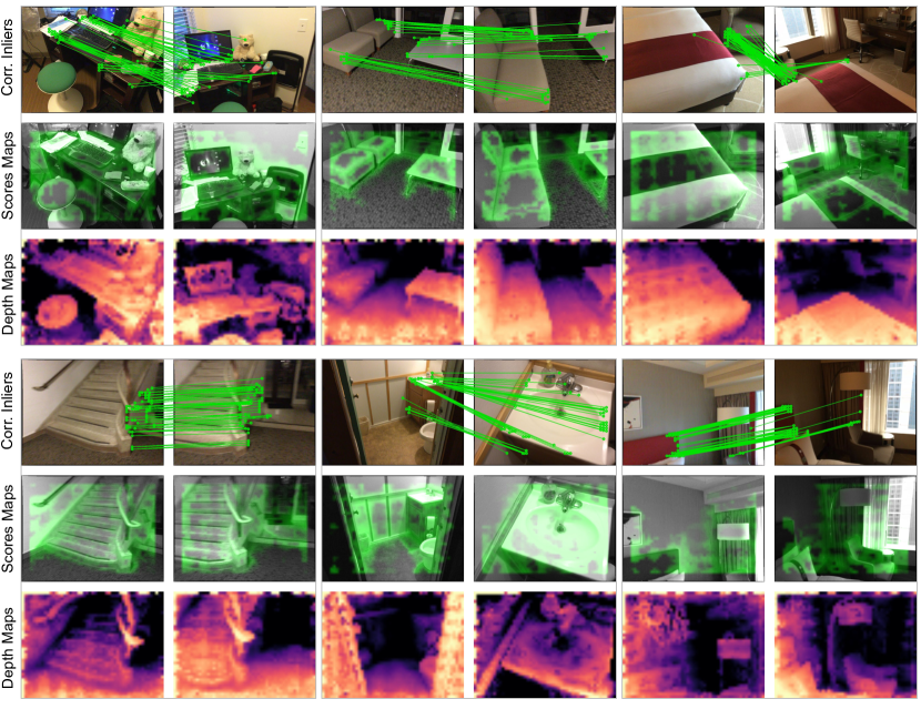
Figure 7: Visual examples on ScanNet dataset. We visualize the inlier correspondences, score, and depth maps predicted by MicKey in ScanNet images. We see that although the images show repetitive patterns and flat areas, MicKey is able to find correct correspondences across views. Besides making our correspondences metric, our depth estimation head provides additional 3D information and geometric constraints to our probabilistic pose solver, making the final decision robust against the mentioned indoor challenges.

Monocular depth evaluation. Table 7 presents monocular depth evaluation metrics for the ScanNet test set, where we have access to GT depths. For completeness, besides DPT [65] and PlaneRCNN [53], we also evaluate the depth estimations of recent ZoeDepth [9]. MicKey-Sc corresponds to evaluating the depth estimates only on the positions where MicKey is most confident. Specifically, we take the depth estimations that correspond to the top 50% scoring positions. And therefore, in this setup, we focus on the positions that will be used to compute the metric relative pose between images. We see that our relative pose supervision, even though not using any depth maps during training, allows MicKey to compute accurate depth maps.

Visual examples. We also show some visual examples of the depth maps estimated by MicKey in Figure 7. Moreover, in the figure, we display the inlier correspondences and the score maps that MicKey computes for each input image. We see that MicKey finds high scoring keypoints in structures beyond corners or blobs, establishing correct matches in images where there are few discriminative structures.

C.2 Map-free

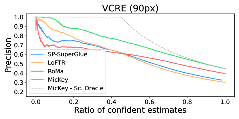
Figure 8: Precision vs ratio of estimates. In this plot, the pose estimates are ranked by the confidence values of the methods, e.g., inlier counting. The Map-free benchmark computes the AUC of the curves to also evaluate the ability of the methods to decide whether their poses should be trusted or not. We plot MicKey- Score (Sc.) Oracle, which corresponds to the curve that MicKey would obtain if its pose confidences were perfect.

Method Confidence tells when we can or not trust a pose estimate. Map-free benchmark evaluates the confidence of the methods via the area under the curve (AUC) metric. The benchmark ranks the poses by confidence, and hence, the AUC is only maximized when the most accurate poses are ranked first. In Figure 8, we visualize the precision versus the ratio of estimates in the validation set scenes, where ground truth poses are available. All matching methods use their inlier counting as their confidence value, meanwhile, MicKey relies on the soft-inlier counting. MicKey’s confidence, hence, is entangled within its training pipeline and directly optimized to be correlated with the quality of its pose predictions. From Figure 8, we see that MicKey obtains the highest number of correctly ranked images before assigning a high score to an invalid pose, where an invalid pose refers to a relative pose with a VCRE higher than 90 pixels. Contrary, as seen in the plot, the second best method, RoMa [25], struggles to rank its pose estimates. I.e., RoMa accepts incorrect poses (VCRE > 90px) as its most confidence estimates. This indicates that RoMa’s poses, although very accurate, do not have a valid mechanism to decide whether they should be trusted or rejected, making them unreliable in an AR application [2].

Map-free Dataset
		VCRE (90px)		Pose (25cm, 5°)
		AUC	Prec. (%)	AUC	Prec. (%)
D+O+P Signal
SuperGlue [22, 69]		0.60	36.1	0.35	16.8
LightGlue [81, 52]		0.53	33.2	0.31	15.8
DeDoDe [26]		0.53	31.2	0.26	12.5
LoFTR [73]		0.61	34.7	0.35	15.4
ASpanFormer [17]		0.64	36.9	0.36	16.3
RoMa [25]		0.67	45.6	0.41	22.8
O+P Signal
RPR [R(6D) + t] [2]		0.40	40.2	0.06	6.0
MicKey-O (ours)		0.75	49.2	0.33	13.3
Pose Signal
RPR [R(6D) + t]		0.18	18.1	0.01	0.6
MicKey (ours)		0.74	49.2	0.28	12.0

Table 8: Additional metrics on Map-free dataset. Besides the VCRE results, we also show the AUC and precision values for a very fine threshold (pose errors at 25cm and 5°).

Pose Metrics. Besides the experiments from the main paper in Map-free, we provide additional metrics in Table 8. Map-free benchmark, although it focuses on the VCRE metric for evaluating algorithms for an AR experience, it also computes the AUC and precision error pose under a very fine threshold (pose error < 25cm, 5°). Under such conditions, all methods have a small AUC and precision value, and hence, applications built on that restrictive threshold would need to discard most of the relative pose estimates. Even though, it gives some possible directions for future work, where one could focus on improving MicKey’s predictions under such strict thresholds.

Pose Solvers. Arnold et al. [2] propose different strategies for recovering the metric scale from the keypoint correspondences. In the first strategy, authors first compute the essential matrix and then rely on the depth estimation to obtain the scaled translation vector (Ess. Scale) [62, 30]. Their second strategy consisted of using the depth maps to lift the 2D keypoints to 3D, and then applying the Perspective-n-Point (PnP) algorithm [31]. We refer to [2] for more details. We compare such strategies in Table 9. Moreover, we also show MicKey’s results with the two different proposed solvers. We demonstrate that obtaining poses with the same probabilistic approach we use during training yields the best results, proving the effectiveness of both, the end-to-end strategy and our probabilistic formulation of the metric relative pose estimation.

Map-free Dataset
		VCRE (90px)			Pose (25cm, 5°)
		AUC	Prec. (%)		AUC	Prec. (%)
Pose Solvers
SuperGlue [22, 69]
Ess. Scale		0.60	36.1		0.35	16.8
PnP		0.60	36.0		0.25	10.7
LoFTR [73]
Ess. Scale		0.61	34.7		0.35	15.4
PnP		0.62	33.4		0.27	9.8
MicKey w/ Overlap
Ess. Scale		0.66	39.3		0.22	8.4
PnP		0.70	42.1		0.36	14.6
Our Solver		0.75	49.2		0.33	13.3
MicKey
Ess. Scale		0.65	37.1		0.20	6.9
PnP		0.70	42.5		0.33	12.8
Our Solver		0.74	49.2		0.28	12.0

Table 9: Pose solver ablation on Map-free. Results show that state-of-the-art matchers work better when estimating the essential matrix from 2D-2D correspondences, and then recovering the metric scale from the depth predictor. MicKey, meanwhile, obtains the top VCRE results when recovering the pose with the probabilistic solver used during training.

Cross-dataset evaluation. We also test the generalization capability of MicKey when trained and tested in different scenarios. We use MicKey trained in ScanNet dataset and evaluate it in the Map-free evaluation. Even though this experiment involves a significant distribution gap (indoor vs. outdoor), MicKey achieves an AUC (VCRE) score of 0.55, still outperforming DISK [81], SiLK [33], and DeDoDe [26], which all were trained on outdoor datasets (see Table 8 for all AUC (VCRE) results).

	DIML Outdoor [46]				DIODE Outdoor [82]
	$\delta_{1}$ $\uparrow$	REL $\downarrow$	RMSE $\downarrow$		$\delta_{1}$ $\uparrow$	REL $\downarrow$	RMSE $\downarrow$
ZoeDepth [9]	0.29	0.64	3.61		0.21	0.76	7.57
MicKey	0.65	0.20	4.30		0.04	0.67	15.18
MicKey-Sc	0.70	0.17	2.39		0.04	0.66	13.76

Table 10: Outdoor monocular depth evaluation. We report the zero-shot generalization on outdoor datasets and see that MicKey provides competitive results even though it was not designed for this task.

Monocular depth estimation. In Table 10, we further evaluate the generalization capabilities of our network also in the zero-shot monocular depth estimation task. We compute its accuracy in the DIML Outdoor [46] and the DIODE Outdoor [82] datasets. As a reference, we also provide ZoeDepth (NK) metrics. Similar to Section C.1 (Table 7), we also show results for MicKey-Sc, where we evaluate depth prediction on the positions where MicKey is most confident (50% top scoring positions). MicKey has been trained with pedestrian smartphone images, and still, it can generalize and produce valid depth maps in datasets with different statistics, or visual conditions.

Map-free Dataset
		VCRE		Median Errors
		AUC / Prec. (%)		Rep. / Trans / Rot
Hard pairs
SuperGlue [22, 69]		0.07 / 3.5		271.8 / 4.5 / 81.6
LoFTR [73]		0.06 / 2.6		255.7 / 4.8 / 88.5
RoMa [25]		0.08 / 7.3		241.7 / 3.1 / 58.3
MicKey (ours)		0.15 / 11.1		233.7 / 3.7 / 75.2

Table 11: Hard examples on the Map-free dataset. We evaluate image pairs from the validation set that are taken under large viewpoint changes. We define such examples as image pairs that are at least 3m apart and have a 45° change in the camera direction. We report the VCRE metrics and the median errors of the estimated poses.

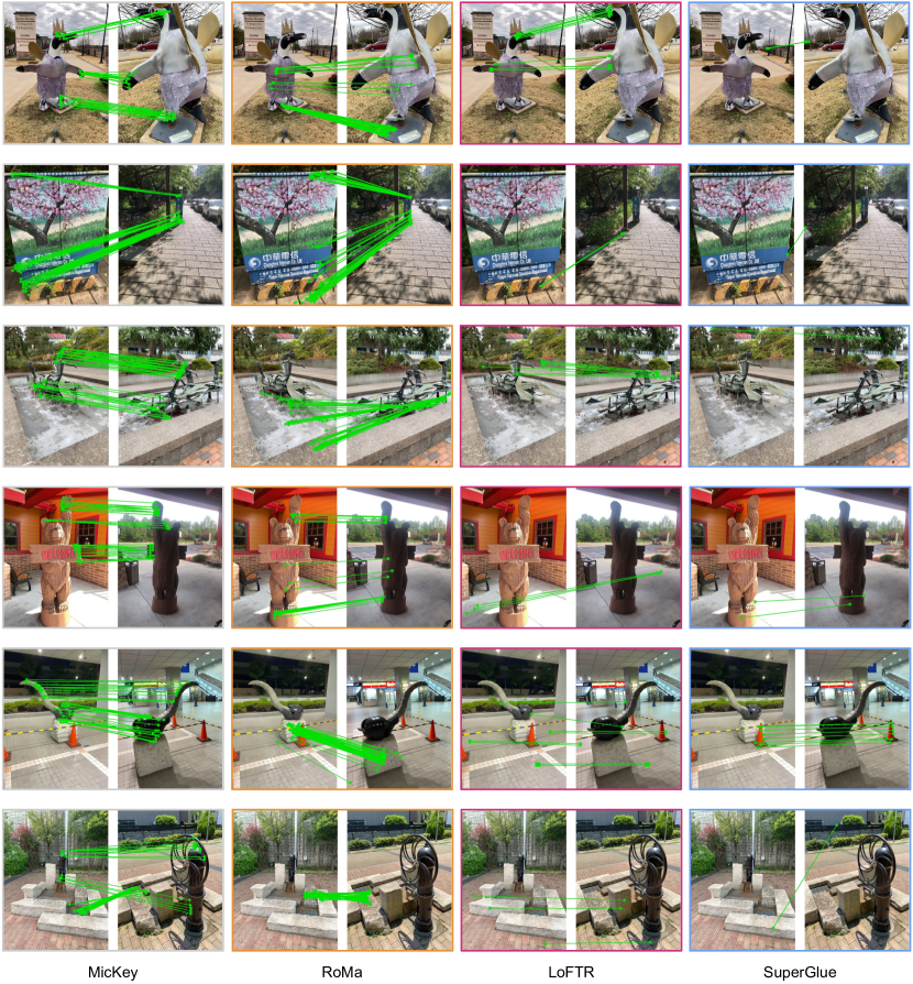
Figure 9: Inlier correspondences on Map-free dataset. We show the inlier correspondences returned by different feature extractors and their pose solvers. MicKey outperforms the other matchers when there are strong viewpoint changes between the two input images. MicKey embeds in a single neural network a feature representation of the keypoints, as well as their 3D geometry, allowing it to match keypoints where little overlap is observed. We see that SuperGlue [22, 69], a sparse feature method like MicKey, struggles to compute good correspondences when images present this kind of extreme viewpoint differences.

Inlier correspondences. In this last section, we show different visual examples in Figure 9. We plot the inlier correspondences that every method returns after computing the relative pose estimation. We observe that MicKey finds correct correspondences even though images were taken from extremely different viewpoints. Moreover, we see that MicKey detects and tries to match the object of interest within the image instead of relying on local patterns that might not appear in the two images. For instance, in images from row 1 or row 4, the object of interest is shown in the images from opposite views, i.e., images were taken with almost a 180° difference. Even so, MicKey is able to match the correct side of the object to its corresponding part in the other image. Thus, we observe that the network is able to reason about the shape of the object and establish correspondences beyond local patterns. RoMa [25] is also able to find good matches, but it fails when the images do not have direct visual overlap. Contrary to LoFTR [73] or RoMA [25], MicKey and SuperGlue [69] are sparse feature methods, and then they only have access to a single image when computing their keypoints and descriptors. Contrary to MicKey, we note that state-of-the-art sparse feature methods (e.g., SuperPoint [22]-SuperGlue [69]) do not find any good correspondences under such extreme cases.

We report the VCRE metrics and median errors on image pairs that have large and challenging viewpoint differences in Table 11. We use the validation scenes, where ground truth data is provided and hence, we can define the difficulty of an image pair. We rely on the pose difference between the reference and the query frame instead of the overlap score, such that unsolvable pairs are also evaluated. We define a hard example as a pair that is taken at least 3 meters apart and with their camera directions being at least rotated by 45°. We see that on those challenging examples, MicKey obtains the highest number of relative poses under the VCRE threshold (90 pixels).

References

- Agarap [2018] Abien Fred Agarap. Deep learning using rectified linear units (ReLU). arXiv preprint arXiv:1803.08375, 2018.
- Arnold et al. [2022] Eduardo Arnold, Jamie Wynn, Sara Vicente, Guillermo Garcia-Hernando, Áron Monszpart, Victor Adrian Prisacariu, Daniyar Turmukhambetov, and Eric Brachmann. Map-free visual relocalization: Metric pose relative to a single image. Proceedings of the European Conference on Computer Vision (ECCV), 2022.
- Avetisyan et al. [2019] Armen Avetisyan, Angela Dai, and Matthias Nießner. End-to-end cad model retrieval and 9dof alignment in 3d scans. In Proceedings of the IEEE/CVF International Conference on computer vision, pages 2551–2560, 2019.
- Balntas et al. [2018] Vassileios Balntas, Shuda Li, and Victor Prisacariu. Relocnet: Continuous metric learning relocalisation using neural nets. In Proceedings of the European Conference on Computer Vision (ECCV), pages 751–767, 2018.
- Barroso-Laguna et al. [2019] Axel Barroso-Laguna, Edgar Riba, Daniel Ponsa, and Krystian Mikolajczyk. Key.Net: Keypoint detection by handcrafted and learned CNN filters. In Proceedings of the IEEE/CVF international conference on computer vision, pages 5836–5844, 2019.
- Barroso-Laguna et al. [2020] Axel Barroso-Laguna, Yannick Verdie, Benjamin Busam, and Krystian Mikolajczyk. HDD-Net: Hybrid detector descriptor with mutual interactive learning. In Proceedings of the Asian Conference on Computer Vision, 2020.
- Barroso-Laguna et al. [2022] Axel Barroso-Laguna, Yurun Tian, and Krystian Mikolajczyk. ScaleNet: A shallow architecture for scale estimation. In Proceedings of the IEEE/CVF Conference on Computer Vision and Pattern Recognition, pages 12808–12818, 2022.
- Barroso-Laguna et al. [2023] Axel Barroso-Laguna, Eric Brachmann, Victor Adrian Prisacariu, Gabriel J Brostow, and Daniyar Turmukhambetov. Two-view geometry scoring without correspondences. In Proceedings of the IEEE/CVF Conference on Computer Vision and Pattern Recognition, pages 8979–8989, 2023.
- Bhat et al. [2023] Shariq Farooq Bhat, Reiner Birkl, Diana Wofk, Peter Wonka, and Matthias Müller. ZoeDepth: Zero-shot transfer by combining relative and metric depth. arXiv preprint arXiv:2302.12288, 2023.
- Bhowmik et al. [2020] Aritra Bhowmik, Stefan Gumhold, Carsten Rother, and Eric Brachmann. Reinforced feature points: Optimizing feature detection and description for a high-level task. In Proceedings of the IEEE/CVF conference on computer vision and pattern recognition, pages 4948–4957, 2020.
- Brachmann and Rother [2018] Eric Brachmann and Carsten Rother. Learning less is more - 6D camera localization via 3D surface regression. In Proceedings of the IEEE conference on computer vision and pattern recognition, pages 4654–4662, 2018.
- Brachmann and Rother [2019] Eric Brachmann and Carsten Rother. Neural-guided RANSAC: Learning where to sample model hypotheses. In Proceedings of the IEEE/CVF International Conference on Computer Vision, pages 4322–4331, 2019.
- Brachmann and Rother [2021] Eric Brachmann and Carsten Rother. Visual camera re-localization from RGB and RGB-D images using DSAC. IEEE transactions on pattern analysis and machine intelligence, 44(9):5847–5865, 2021.
- Brachmann et al. [2017] Eric Brachmann, Alexander Krull, Sebastian Nowozin, Jamie Shotton, Frank Michel, Stefan Gumhold, and Carsten Rother. DSAC - differentiable ransac for camera localization. In Proceedings of the IEEE conference on computer vision and pattern recognition, pages 6684–6692, 2017.
- Cai et al. [2021] Ruojin Cai, Bharath Hariharan, Noah Snavely, and Hadar Averbuch-Elor. Extreme rotation estimation using dense correlation volumes. In Proceedings of the IEEE/CVF Conference on Computer Vision and Pattern Recognition, pages 14566–14575, 2021.
- Cavalli et al. [2020] Luca Cavalli, Viktor Larsson, Martin Ralf Oswald, Torsten Sattler, and Marc Pollefeys. AdaLAM: Revisiting handcrafted outlier detection. arXiv preprint arXiv:2006.04250, 2020.
- Chen et al. [2022] Hongkai Chen, Zixin Luo, Lei Zhou, Yurun Tian, Mingmin Zhen, Tian Fang, David Mckinnon, Yanghai Tsin, and Long Quan. ASpanFormer: Detector-Free image matching with adaptive span transformer. In European Conference on Computer Vision, pages 20–36. Springer, 2022.
- Chen et al. [2021] Kefan Chen, Noah Snavely, and Ameesh Makadia. Wide-baseline relative camera pose estimation with directional learning. In Proceedings of the IEEE/CVF Conference on Computer Vision and Pattern Recognition, pages 3258–3268, 2021.
- Christiansen et al. [2019] Peter Hviid Christiansen, Mikkel Fly Kragh, Yury Brodskiy, and Henrik Karstoft. UnSuperpoint: End-to-end unsupervised interest point detector and descriptor. arXiv preprint arXiv:1907.04011, 2019.
- Chum and Matas [2005] Ondrej Chum and Jiri Matas. Matching with PROSAC-progressive sample consensus. In 2005 IEEE computer society conference on computer vision and pattern recognition (CVPR’05), pages 220–226. IEEE, 2005.
- Dai et al. [2017] Angela Dai, Angel X Chang, Manolis Savva, Maciej Halber, Thomas Funkhouser, and Matthias Nießner. ScanNet: Richly-annotated 3d reconstructions of indoor scenes. In Proceedings of the IEEE conference on computer vision and pattern recognition, pages 5828–5839, 2017.
- DeTone et al. [2018] Daniel DeTone, Tomasz Malisiewicz, and Andrew Rabinovich. SuperPoint: Self-supervised interest point detection and description. In Proceedings of the IEEE conference on computer vision and pattern recognition workshops, pages 224–236, 2018.
- Ding et al. [2020] Zihan Ding, Yanhua Huang, Hang Yuan, and Hao Dong. Introduction to reinforcement learning. Deep reinforcement learning: fundamentals, research and applications, pages 47–123, 2020.
- Dusmanu et al. [2019] Mihai Dusmanu, Ignacio Rocco, Tomas Pajdla, Marc Pollefeys, Josef Sivic, Akihiko Torii, and Torsten Sattler. D2-Net: A trainable CNN for joint detection and description of local features. arXiv preprint arXiv:1905.03561, 2019.
- Edstedt et al. [2023] Johan Edstedt, Qiyu Sun, Georg Bökman, Mårten Wadenbäck, and Michael Felsberg. RoMa: Revisiting Robust Losses for Dense Feature Matching. arXiv preprint arXiv:2305.15404, 2023.
- Edstedt et al. [2024] Johan Edstedt, Georg Bökman, Mårten Wadenbäck, and Michael Felsberg. DeDoDe: Detect, Don’t Describe – Describe, Don’t Detect for Local Feature Matching. International Conference on 3D Vision (3DV), 2024.
- Eggert et al. [1997] David W Eggert, Adele Lorusso, and Robert B Fisher. Estimating 3D rigid body transformations: a comparison of four major algorithms. Machine vision and applications, 9(5-6):272–290, 1997.
- Eigen et al. [2014] David Eigen, Christian Puhrsch, and Rob Fergus. Depth map prediction from a single image using a multi-scale deep network. Advances in neural information processing systems, 27, 2014.
- Fathy et al. [2011] Mohammed E Fathy, Ashraf S Hussein, and Mohammed F Tolba. Fundamental matrix estimation: A study of error criteria. Pattern Recognition Letters, 32(2):383–391, 2011.
- Fischler and Bolles [1981] Martin A Fischler and Robert C Bolles. Random sample consensus: a paradigm for model fitting with applications to image analysis and automated cartography. Communications of the ACM, 24(6):381–395, 1981.
- Gao et al. [2003] Xiao-Shan Gao, Xiao-Rong Hou, Jianliang Tang, and Hang-Fei Cheng. Complete solution classification for the perspective-three-point problem. IEEE transactions on pattern analysis and machine intelligence, 25(8):930–943, 2003.
- Giubilato et al. [2018] Riccardo Giubilato, Sebastiano Chiodini, Marco Pertile, and Stefano Debei. Scale correct monocular visual odometry using a lidar altimeter. In 2018 IEEE/RSJ international conference on intelligent robots and systems (IROS), pages 3694–3700. IEEE, 2018.
- Gleize et al. [2023] Pierre Gleize, Weiyao Wang, and Matt Feiszli. SiLK–Simple Learned Keypoints. Proceedings of the IEEE/CVF international conference on computer vision, 2023.
- Godard et al. [2017] Clément Godard, Oisin Mac Aodha, and Gabriel J Brostow. Unsupervised monocular depth estimation with left-right consistency. In Proceedings of the IEEE conference on computer vision and pattern recognition, pages 270–279, 2017.
- Godard et al. [2019] Clément Godard, Oisin Mac Aodha, Michael Firman, and Gabriel J Brostow. Digging into self-supervised monocular depth estimation. In Proceedings of the IEEE/CVF international conference on computer vision, pages 3828–3838, 2019.
- Hartley and Zisserman [2003] Richard Hartley and Andrew Zisserman. Multiple view geometry in computer vision. Cambridge university press, 2003.
- Ioffe and Szegedy [2015] Sergey Ioffe and Christian Szegedy. Batch normalization: Accelerating deep network training by reducing internal covariate shift. In International conference on machine learning, pages 448–456. PMLR, 2015.
- Jang et al. [2016] Eric Jang, Shixiang Gu, and Ben Poole. Categorical reparameterization with gumbel-softmax. arXiv preprint arXiv:1611.01144, 2016.
- Jiang et al. [2021] Wei Jiang, Eduard Trulls, Jan Hosang, Andrea Tagliasacchi, and Kwang Moo Yi. COTR: Correspondence transformer for matching across images. In Proceedings of the IEEE/CVF International Conference on Computer Vision, pages 6207–6217, 2021.
- Jin et al. [2021] Yuhe Jin, Dmytro Mishkin, Anastasiia Mishchuk, Jiri Matas, Pascal Fua, Kwang Moo Yi, and Eduard Trulls. Image matching across wide baselines: From paper to practice. International Journal of Computer Vision, 129(2):517–547, 2021.
- Kabsch [1976] Wolfgang Kabsch. A solution for the best rotation to relate two sets of vectors. Acta Crystallographica Section A: Crystal Physics, Diffraction, Theoretical and General Crystallography, 32(5):922–923, 1976.
- Katharopoulos et al. [2020] Angelos Katharopoulos, Apoorv Vyas, Nikolaos Pappas, and François Fleuret. Transformers are RNNs: Fast autoregressive transformers with linear attention. In International Conference on Machine Learning, pages 5156–5165. PMLR, 2020.
- Kendall and Cipolla [2017] Alex Kendall and Roberto Cipolla. Geometric loss functions for camera pose regression with deep learning. In Proceedings of the IEEE conference on computer vision and pattern recognition, pages 5974–5983, 2017.
- Kendall et al. [2015] Alex Kendall, Matthew Grimes, and Roberto Cipolla. Posenet: A convolutional network for real-time 6-dof camera relocalization. In Proceedings of the IEEE international conference on computer vision, pages 2938–2946, 2015.
- Khatib et al. [2022] Fadi Khatib, Yuval Margalit, Meirav Galun, and Ronen Basri. Grelpose: Generalizable end-to-end relative camera pose regression. arXiv preprint arXiv:2211.14950, 2022.
- Kim et al. [2018] Youngjung Kim, Hyungjoo Jung, Dongbo Min, and Kwanghoon Sohn. Deep monocular depth estimation via integration of global and local predictions. IEEE transactions on Image Processing, 27(8):4131–4144, 2018.
- Kingma and Ba [2014] Diederik P Kingma and Jimmy Ba. Adam: A method for stochastic optimization. arXiv preprint arXiv:1412.6980, 2014.
- Lenc and Vedaldi [2016] Karel Lenc and Andrea Vedaldi. Learning covariant feature detectors. In Computer Vision–ECCV 2016 Workshops: Amsterdam, The Netherlands, October 8-10 and 15-16, 2016, Proceedings, Part III 14, pages 100–117. Springer, 2016.
- Li et al. [2022] Kunhong Li, Longguang Wang, Li Liu, Qing Ran, Kai Xu, and Yulan Guo. Decoupling makes weakly supervised local feature better. In Proceedings of the IEEE/CVF Conference on Computer Vision and Pattern Recognition, pages 15838–15848, 2022.
- Li et al. [2020] Xiaotian Li, Shuzhe Wang, Yi Zhao, Jakob Verbeek, and Juho Kannala. Hierarchical scene coordinate classification and regression for visual localization. In Proceedings of the IEEE/CVF Conference on Computer Vision and Pattern Recognition, pages 11983–11992, 2020.
- Li and Snavely [2018] Zhengqi Li and Noah Snavely. MegaDepth: Learning single-view depth prediction from internet photos. In Proceedings of the IEEE conference on computer vision and pattern recognition, pages 2041–2050, 2018.
- Lindenberger et al. [2023] Philipp Lindenberger, Paul-Edouard Sarlin, and Marc Pollefeys. LightGlue: Local feature matching at light speed. arXiv preprint arXiv:2306.13643, 2023.
- Liu et al. [2019] Chen Liu, Kihwan Kim, Jinwei Gu, Yasutaka Furukawa, and Jan Kautz. PlaneRCNN: 3d plane detection and reconstruction from a single image. In Proceedings of the IEEE/CVF Conference on Computer Vision and Pattern Recognition, pages 4450–4459, 2019.
- Lowe [1999] David G Lowe. Object recognition from local scale-invariant features. In Proceedings of the seventh IEEE international conference on computer vision, pages 1150–1157. Ieee, 1999.
- Luo et al. [2020] Zixin Luo, Lei Zhou, Xuyang Bai, Hongkai Chen, Jiahui Zhang, Yao Yao, Shiwei Li, Tian Fang, and Long Quan. Aslfeat: Learning local features of accurate shape and localization. In Proceedings of the IEEE/CVF conference on computer vision and pattern recognition, pages 6589–6598, 2020.
- Ma et al. [2021] Jiayi Ma, Xingyu Jiang, Aoxiang Fan, Junjun Jiang, and Junchi Yan. Image matching from handcrafted to deep features: A survey. International Journal of Computer Vision, 129:23–79, 2021.
- Mikolajczyk and Schmid [2004] Krystian Mikolajczyk and Cordelia Schmid. Scale & affine invariant interest point detectors. International journal of computer vision, 60:63–86, 2004.
- Mikolajczyk et al. [2005] Krystian Mikolajczyk, Tinne Tuytelaars, Cordelia Schmid, Andrew Zisserman, Jiri Matas, Frederik Schaffalitzky, Timor Kadir, and L Van Gool. A comparison of affine region detectors. International journal of computer vision, 65:43–72, 2005.
- Mishkin et al. [2018] Dmytro Mishkin, Filip Radenovic, and Jiri Matas. Repeatability is not enough: Learning affine regions via discriminability. In Proceedings of the European Conference on Computer Vision (ECCV), pages 284–300, 2018.
- Narvekar et al. [2020] Sanmit Narvekar, Bei Peng, Matteo Leonetti, Jivko Sinapov, Matthew E Taylor, and Peter Stone. Curriculum learning for reinforcement learning domains: A framework and survey. The Journal of Machine Learning Research, 21(1):7382–7431, 2020.
- Nie et al. [2023] Chang Nie, Guangming Wang, Zhe Liu, Luca Cavalli, Marc Pollefeys, and Hesheng Wang. Rlsac: Reinforcement learning enhanced sample consensus for end-to-end robust estimation. In Proceedings of the IEEE/CVF International Conference on Computer Vision, pages 9891–9900, 2023.
- Nistér [2004] David Nistér. An efficient solution to the five-point relative pose problem. IEEE transactions on pattern analysis and machine intelligence, 26(6):756–770, 2004.
- Nützi et al. [2011] Gabriel Nützi, Stephan Weiss, Davide Scaramuzza, and Roland Siegwart. Fusion of imu and vision for absolute scale estimation in monocular slam. Journal of intelligent & robotic systems, 61(1-4):287–299, 2011.
- Oquab et al. [2023] Maxime Oquab, Timothée Darcet, Théo Moutakanni, Huy Vo, Marc Szafraniec, Vasil Khalidov, Pierre Fernandez, Daniel Haziza, Francisco Massa, Alaaeldin El-Nouby, et al. Dinov2: Learning robust visual features without supervision. arXiv preprint arXiv:2304.07193, 2023.
- Ranftl et al. [2021] René Ranftl, Alexey Bochkovskiy, and Vladlen Koltun. Vision transformers for dense prediction. In Proceedings of the IEEE/CVF international conference on computer vision, pages 12179–12188, 2021.
- Revaud et al. [2019] Jerome Revaud, Philippe Weinzaepfel, César De Souza, Noe Pion, Gabriela Csurka, Yohann Cabon, and Martin Humenberger. R2D2: repeatable and reliable detector and descriptor. arXiv preprint arXiv:1906.06195, 2019.
- Roessle and Nießner [2023] Barbara Roessle and Matthias Nießner. End2End Multi-View Feature Matching with Differentiable Pose Optimization. In Proceedings of the IEEE/CVF International Conference on Computer Vision, pages 477–487, 2023.
- Santellani et al. [2023] Emanuele Santellani, Christian Sormann, Mattia Rossi, Andreas Kuhn, and Friedrich Fraundorfer. S-TREK: Sequential translation and rotation equivariant keypoints for local feature extraction. In Proceedings of the IEEE/CVF International Conference on Computer Vision, pages 9728–9737, 2023.
- Sarlin et al. [2020] Paul-Edouard Sarlin, Daniel DeTone, Tomasz Malisiewicz, and Andrew Rabinovich. SuperGlue: Learning feature matching with graph neural networks. In Proceedings of the IEEE/CVF conference on computer vision and pattern recognition, pages 4938–4947, 2020.
- Shavit et al. [2021] Yoli Shavit, Ron Ferens, and Yosi Keller. Learning multi-scene absolute pose regression with transformers. In Proceedings of the IEEE/CVF International Conference on Computer Vision, pages 2733–2742, 2021.
- Shotton et al. [2013] Jamie Shotton, Ben Glocker, Christopher Zach, Shahram Izadi, Antonio Criminisi, and Andrew Fitzgibbon. Scene coordinate regression forests for camera relocalization in rgb-d images. In Proceedings of the IEEE conference on computer vision and pattern recognition, pages 2930–2937, 2013.
- Spencer et al. [2023] Jaime Spencer, Chris Russell, Simon Hadfield, and Richard Bowden. Kick back & relax: Learning to reconstruct the world by watching slowtv. In Proceedings of the IEEE/CVF International Conference on Computer Vision, 2023.
- Sun et al. [2021] Jiaming Sun, Zehong Shen, Yuang Wang, Hujun Bao, and Xiaowei Zhou. LoFTR: Detector-free local feature matching with transformers. In Proceedings of the IEEE/CVF conference on computer vision and pattern recognition, pages 8922–8931, 2021.
- Sun et al. [2020] Weiwei Sun, Wei Jiang, Eduard Trulls, Andrea Tagliasacchi, and Kwang Moo Yi. ACNe: Attentive context normalization for robust permutation-equivariant learning. In Proceedings of the IEEE/CVF Conference on Computer Vision and Pattern Recognition, pages 11286–11295, 2020.
- Tateno et al. [2017] Keisuke Tateno, Federico Tombari, Iro Laina, and Nassir Navab. CNN-SLAM: Real-time dense monocular slam with learned depth prediction. In Proceedings of the IEEE conference on computer vision and pattern recognition, pages 6243–6252, 2017.
- Tian et al. [2019] Yurun Tian, Xin Yu, Bin Fan, Fuchao Wu, Huub Heijnen, and Vassileios Balntas. SOSNet: Second order similarity regularization for local descriptor learning. In Proceedings of the IEEE/CVF Conference on Computer Vision and Pattern Recognition, pages 11016–11025, 2019.
- Tian et al. [2020] Yurun Tian, Axel Barroso Laguna, Tony Ng, Vassileios Balntas, and Krystian Mikolajczyk. HyNet: Learning local descriptor with hybrid similarity measure and triplet loss. Advances in Neural Information Processing Systems, 33:7401–7412, 2020.
- Torr and Zisserman [2000] Philip HS Torr and Andrew Zisserman. MLESAC: A new robust estimator with application to estimating image geometry. Computer vision and image understanding, 78(1):138–156, 2000.
- Torr et al. [2002] Philip Hilaire Torr, Slawomir J Nasuto, and John Mark Bishop. NAPSAC: High noise, high dimensional robust estimation-it’s in the bag. In British Machine Vision Conference (BMVC), page 3, 2002.
- Truong et al. [2021] Prune Truong, Martin Danelljan, Luc Van Gool, and Radu Timofte. Learning accurate dense correspondences and when to trust them. In Proceedings of the IEEE/CVF Conference on Computer Vision and Pattern Recognition, pages 5714–5724, 2021.
- Tyszkiewicz et al. [2020] Michał Tyszkiewicz, Pascal Fua, and Eduard Trulls. DISK: Learning local features with policy gradient. Advances in Neural Information Processing Systems, 33:14254–14265, 2020.
- Vasiljevic et al. [2019] Igor Vasiljevic, Nick Kolkin, Shanyi Zhang, Ruotian Luo, Haochen Wang, Falcon Z Dai, Andrea F Daniele, Mohammadreza Mostajabi, Steven Basart, Matthew R Walter, et al. DIODE: A dense indoor and outdoor depth dataset. arXiv preprint arXiv:1908.00463, 2019.
- Verdie et al. [2015] Yannick Verdie, Kwang Yi, Pascal Fua, and Vincent Lepetit. TILDE: A temporally invariant learned detector. In Proceedings of the IEEE conference on computer vision and pattern recognition, pages 5279–5288, 2015.
- Watson et al. [2019] Jamie Watson, Michael Firman, Gabriel J Brostow, and Daniyar Turmukhambetov. Self-supervised monocular depth hints. In Proceedings of the IEEE/CVF International Conference on Computer Vision, pages 2162–2171, 2019.
- Wei et al. [2023] Tong Wei, Yash Patel, Alexander Shekhovtsov, Jiri Matas, and Daniel Barath. Generalized differentiable RANSAC. In Proceedings of the IEEE/CVF International Conference on Computer Vision, pages 17649–17660, 2023.
- Williams [1992] Ronald J Williams. Simple statistical gradient-following algorithms for connectionist reinforcement learning. Machine learning, 8:229–256, 1992.
- Winkelbauer et al. [2021] Dominik Winkelbauer, Maximilian Denninger, and Rudolph Triebel. Learning to localize in new environments from synthetic training data. In 2021 IEEE International Conference on Robotics and Automation (ICRA), pages 5840–5846. IEEE, 2021.
- Yi et al. [2016] Kwang Moo Yi, Yannick Verdie, Pascal Fua, and Vincent Lepetit. Learning to assign orientations to feature points. In Proceedings of the IEEE conference on computer vision and pattern recognition, pages 107–116, 2016.
- Yi et al. [2018] Kwang Moo Yi, Eduard Trulls, Yuki Ono, Vincent Lepetit, Mathieu Salzmann, and Pascal Fua. Learning to find good correspondences. In Proceedings of the IEEE conference on computer vision and pattern recognition, pages 2666–2674, 2018.
- Yin and Shi [2018] Zhichao Yin and Jianping Shi. Geonet: Unsupervised learning of dense depth, optical flow and camera pose. In Proceedings of the IEEE conference on computer vision and pattern recognition, pages 1983–1992, 2018.
- Zhang et al. [2019] Jiahui Zhang, Dawei Sun, Zixin Luo, Anbang Yao, Lei Zhou, Tianwei Shen, Yurong Chen, Long Quan, and Hongen Liao. Learning two-view correspondences and geometry using order-aware network. In Proceedings of the IEEE/CVF international conference on computer vision, pages 5845–5854, 2019.
- Zhao et al. [2019] Chen Zhao, Zhiguo Cao, Chi Li, Xin Li, and Jiaqi Yang. NM-Net: Mining reliable neighbors for robust feature correspondences. In Proceedings of the IEEE/CVF Conference on Computer Vision and Pattern Recognition, pages 215–224, 2019.
- Zou et al. [2018] Yuliang Zou, Zelun Luo, and Jia-Bin Huang. DF-Net: Unsupervised joint learning of depth and flow using cross-task consistency. In Proceedings of the European conference on computer vision (ECCV), pages 36–53, 2018.